
How To Use Excel:
A Beginner’s Guide To Getting Started
Written by co-founder Kasper Langmann, Microsoft Office Specialist.
Excel is a powerful application—but it can also be very intimidating.
That’s why we’ve put together this beginner’s guide to getting started with Excel.
It will take you from the very beginning (opening a spreadsheet), through entering and working with data, and finish with saving and sharing.
It’s everything you need to know to get started with Excel.
If you want to tag along as you read, please download the free sample Excel workbook here.
Opening an Excel spreadsheet
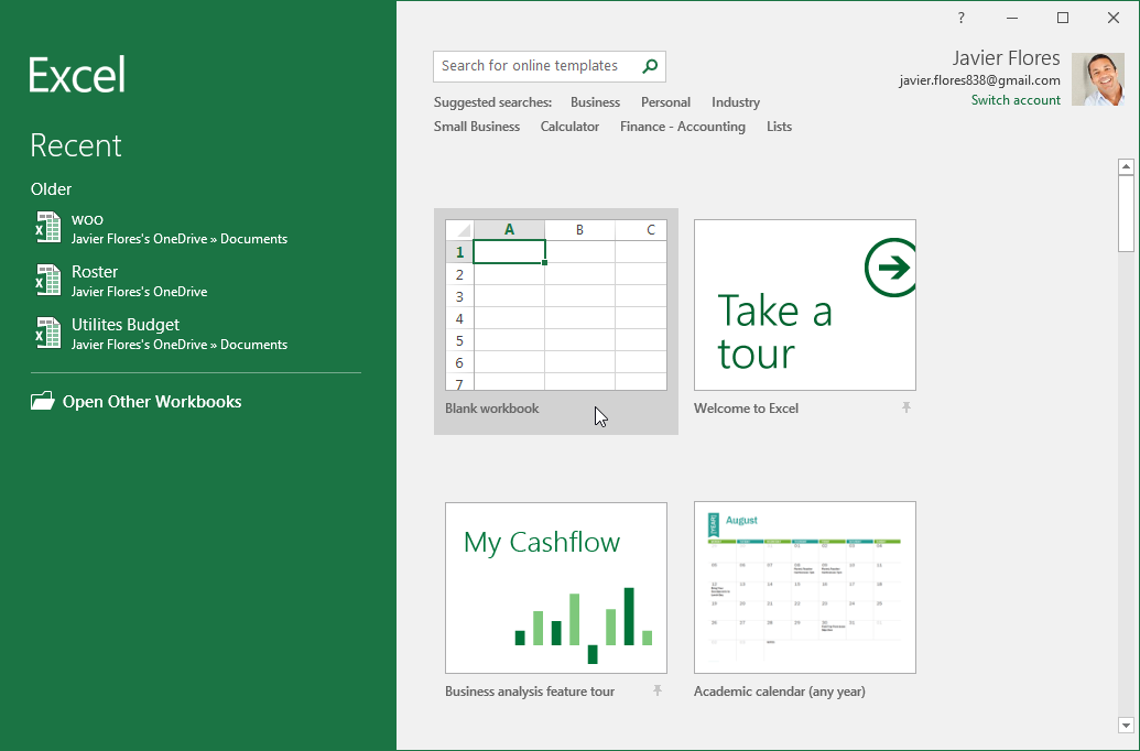
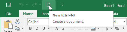
When you first open Excel (by double-clicking the icon or selecting it from the Start menu), the application will ask what you want to do.

If you want to open a new Excel spreadsheet, click Blank workbook.
To open an existing spreadsheet (like the example workbook you just downloaded), click Open Other Workbooks in the lower-left corner, then click Browse on the left side of the resulting window.

Then use the file explorer to find the Excel workbook you’re looking for, select it, and click Open.
Workbooks vs. spreadsheets
There’s something we should clear up before we move on.
A workbook is an Excel file. It usually has a file extension of .XLSX (if you’re using an older version of Excel, it could be .XLS).
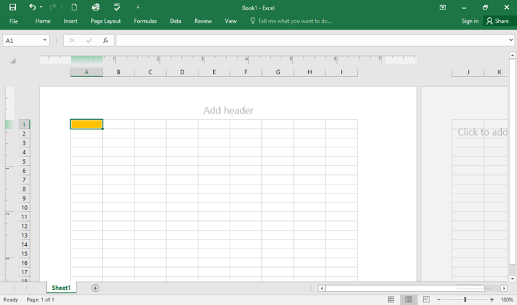
A spreadsheet is a single sheet inside a workbook. There can be many sheets inside of a workbook, and they’re accessed via the tabs at the bottom of the screen.
A spreadsheet (a.k.a. a sheet/tab) contains all the cells you can see and use in the >1 million rows >16,000 columns.
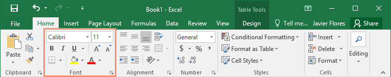
Working with the Ribbon
The Ribbon is the central control panel of Excel. You can do just about everything you need to directly from the Ribbon.
Where is this powerful tool? At the top of the window:

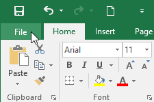
There are a number of tabs, including the File tab, Home tab, Insert tab, Data tab, Review tab, and a few others. Each tab contains different buttons.
Try clicking on a few different tabs to see which buttons appear below them.
 Kasper Langmann, Co-founder of Spreadsheeto
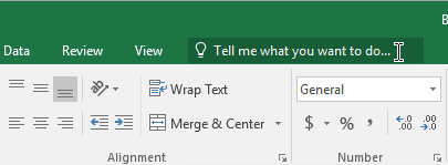
There’s also a very useful search bar in the Ribbon. It says Tell me what you want to do. Just type in what you’re looking for, and Excel will help you find it.

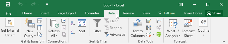
Most of the time, you’ll be in the Home tab of the Ribbon. But Formulas and Data are also very useful (we’ll be talking about formulas shortly).
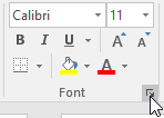
Pro tip: Ribbon sections
In addition to tabs, the Ribbon also has some smaller sections. And when you’re looking for something specific, those sections can help you find it.
For example, if you’re looking for sorting and filtering options, you don’t want to hover over dozens of buttons finding out what they do.
Instead, skim through the section names until you find what you’re looking for:

Managing your sheets
As we saw, workbooks can contain multiple sheets.
You can manage those sheets with the sheet tabs near the bottom of the screen. Click a tab to open that particular worksheet.
If you’re using our example workbook, you’ll see two sheets, called Welcome and Thank You:

To add a new worksheet, click the + (plus) button at the end of the list of sheets.
You can also reorder the sheets in your workbook by dragging them to a new location.
And if you right-click a worksheet tab, you’ll get a number of options:

For now, don’t worry too much about these options. Rename and Delete are useful, but the rest needn’t concern you.
Kasper Langmann, Co-founder of SpreadsheetoEntering data
Now it’s time to enter some data!
And while entering data is one of the most central and important things you can do in Excel, it’s almost effortless.
Just click into a blank cell and start typing.
Go ahead, try it! Type your name, birthday, and your favorite number into some blank cells.
Kasper Langmann, Co-founder of SpreadsheetoYou can also copy (Ctrl + C), cut (Ctrl + X), and paste (Ctrl + V) any data you’d like (or read our full guide on copying and pasting here).
Try copying and pasting the data from multiple cells inthe example spreadsheet into another column.
You can also copy data from other programs into Excel.
Try copying this list of numbers and pasting it into your sheet:
- 17
- 24
- 9
- 00
- 3
- 12
That’s all we’re going to cover for basic data entry. Just know that there are lots of other ways to get data into your spreadsheets if you need them.
Kasper Langmann, Co-founder of SpreadsheetoBasic calculations
Now that we’ve seen how to get some basic data into our spreadsheet, we’re going to do some things with it.
Running basic calculations in Excel is easy. First, we’ll look at how to add two numbers.
Important: start calculations with = (equals)
When you’re running a calculation (or a formula, which we’ll discuss next), the first thing you need to type is an equals sign. This tells Excel to get ready to run some sort of calculation.
So when you see something like =MEDIAN(A2:A51), make sure you type it exactly as it is—including the equals sign.
Let’s add 3 and 4. Type the following formula in a blank cell:
=3+4
Then hit Enter.

When you hit Enter, Excel evaluates your equation and displays the result, 7.
But if you look above at the formula bar, you’ll still see the original formula.
That’s a useful thing to keep in mind, in case you forget what you typed originally.
You can also edit a cell in the formula bar. Click on any cell, then click into the formula bar and start typing.
Kasper Langmann, Co-founder of SpreadsheetoPerforming subtraction, multiplication, and division is just as easy. Try these formulas:
- =4-6
- =2*5
- =-10/3
What we’re going to cover next is one of the most important things in Excel. We’re giving it a very basic overview here, but feel free to read our post on cell references to get the details.
Kasper Langmann, Co-founder of SpreadsheetoNow let’s try something different. Open up the first sheet in the example workbook, click into cell C1, and type the following:
=A1+B1
Hit Enter.
You should get 82, the sum of the numbers in cells A1 and B1.
Now, change one of the numbers in A1 or B1 and watch what happens:
Because you’re adding A1 and B1, Excel automatically updates the total when you change the values in one of those cells.
Try doing different types of arithmetic on the other numbers in columns A and B using this method.
Unlocking the power of functions
Excel’s greatest power lies in functions. These let you run complex calculations with a few keypresses.
We’ll barely scratch the surface of functions here. Check out our other blog posts to see some of the great things you can do with functions!
Kasper Langmann, Co-founder of SpreadsheetoMany formulas take sets of numbers and give you information about them.
For example, the AVERAGE function gives you the average of a set of numbers. Let’s try using it.
Click into an empty cell and type the following formula:
=AVERAGE(A1:A4)
Then hit Enter.

The resulting number, 0.25, is the average of the numbers in cells A1, A2, A3, and A4.
Cell range notation
In the formula above, we used “A1:A4” to tell Excel to look at all the cells between A1 and A4, including both of those cells. You can read it as “A1 through A4.”
You can also use this to include numbers in different columns. “A5:C7” includes A5, A6, A7, B5, B6, B7, C5, C6, and C7.
There are also functions that work on text.
Let’s try the CONCATENATE function!
Click into cell C5 and type this formula:
=CONCATENATE(A5, ” “, B5)
Then hit Enter.
You’ll see the message “Welcome to Spreadsheeto” in the cell.
How did this happen? CONCATENATE takes cells with text in them and puts them together.
We put the contents of A5 and B5 together. But because we also needed a space between “to” and “Spreadsheeto,” we included a third argument: the space between two quotes.
Remember that you can mix cell references (like “A5″) and typed values (like ” “) in formulas.
Kasper Langmann, Co-founder of SpreadsheetoExcel has dozens of useful functions. To find the function that will solve a particular problem, head to the Formulas tab and click on one of the icons:

Scroll through the list of available functions, and select the one you want (you may have to look around for a while).
Then Excel will help you get the right numbers in the right places:

If you start typing a formula, starting with the equals sign, Excel will help you by showing you some possible functions that you might be looking for:

And finally, once you’ve typed the name of a formula and the opening parenthesis, Excel will tell you which arguments need to go where:

If you’ve never used a function before, it might be difficult to interpret Excel’s reminders. But once you get more experience, it’ll become clear.
This is a tiny preview of how functions work and what they can do. It should be enough to get you going on the tasks you need to accomplish right away.
Kasper Langmann, Co-founder of SpreadsheetoSaving and sharing your work
After you’ve done a bunch of work with your spreadsheet, you’re going to want to save your changes.
Hit Ctrl + S to save. If you haven’t yet saved your spreadsheet, you’ll be asked where you want to save it and what you want to call it.
You can also click the Save button in the Quick Access Toolbar:

It’s a good idea to get into the habit of saving often. Trying to recover unsaved changes is a pain!
Kasper Langmann, Co-founder of SpreadsheetoThe easiest way to share your spreadsheets is via OneDrive.
Click the Share button in the top-right corner of the window, and Excel will walk you through sharing your document.

You can also save your document and email it, or use any other cloud service to share it with others.
That’s it – Now what?
This was how to use Excel.
Or… at least a small fraction of it.
Microsoft Excel can be intimidating, but once you get the basics down, it’s easier to learn the more advanced functions.
This was your introduction to “the basics”. So, if you’re not ready to get some advanced Excel knowledge, go ahead and practice with some of the existing data at the office 🧑🏼💻
If you’re ready to take your next steps, go ahead and enroll in my 30-minute free online course where you learn: IF, SUMIF, VLOOKUP, and data cleaning.
These are some of the most important topics of Excel💪🏼
Other resources
Now, you can’t excel at Excel without mastering some of the lookup functions like VLOOKUP and the new XLOOKUP.
But also, you don’t wanna miss out on pivot tables. You can use these to transform your Microsoft Excel data into insightful reports in just a few clicks🤯
Or if you’re into automating Excel spreadsheet formatting, go ahead and read my guide to conditional formatting here.
Kasper Langmann2023-02-23T14:45:07+00:00
Page load link
Содержание
- Start using Excel
- Start using Excel
- Want more?
- Start using Excel
- Start using Excel
- Want more?
- Customize how Excel starts
- Automatically start Excel with a blank workbook
- Automatically open a specific workbook when you start Excel
- Locate the XLStart folder
- Use an alternate startup folder
- Stop a specific workbook from opening when you start Excel
- Automatically open a workbook template or worksheet template when you create a new workbook or worksheet
- Prevent automatic macros from running when you start Excel
Start using Excel

The best way to learn about Excel 2013 is to start using it. Create a blank workbook and learn the basics of working with columns, cells, and data.
Start using Excel
The best way to learn about Excel 2013 is to start using it.
You can open an existing workbook, or start with a template. Then, add some data into cells, use the ribbon, use the mini toolbar.
Want more?
The best way to learn about Excel 2013 is to start using it.
This is what you see when you start Excel for the first time.
You can open an existing workbook over here or start with a template.
Since this is our first time, let’s keep it simple and select Blank workbook.
The area down here is where you create your worksheet.
And you’ll find all the tools you need to work on it, up here, in this area called the ribbon.
In this area, you’ll find the name box and formula bar.
You’ll see what those do as we go along. Now click somewhere in the work area.
These little rectangles, called cells, each hold one piece of information: some text, a number, or a formula.
Let’s say we want to create a worksheet to track expenses on an expansion project.
Type the first budget item, and press Enter.
There are literally millions of cells in a worksheet, but each one can be identified using this grid system of rows and columns.
For example, the address of this cell is C6; column C, row 6.
The name box shows which cell is selected. You’ll see why addresses are important later. Next, type the other budget items.
This is a breakdown of the work required for the expansion project.
If the text doesn’t fit in the cells, come up here, and hold the mouse over the column border until you see a double-headed arrow.
Then, click and drag the border to widen the column.
Now to make our worksheet more interesting, let’s add rough estimates for each work item in the next column.
To make the numbers look like $ amounts, we’ll add some formatting.
First, select the numbers by clicking the first number and dragging the mouse down the list.
The gray highlighting and green border mean the cells are selected.
Right-click the selection, and the right-click menu opens along with this box up here called the mini-toolbar.
The mini-toolbar changes depending on what you select.
In this case, it contains commands for formatting the cells.
Click the $ sign to format the numbers as $ amounts.
Now it is beginning to look more like a worksheet.
To make it official, let’s add a header row up here, so that anyone who looks at the worksheet will know what the data means in each column.
Next, let’s do something to the data to make it easier to work with.
Select the header and data. Click the top left corner, and drag the mouse to the bottom right.
This time, instead of right-clicking, just hold the mouse over the selection, and a button appears.
Click it and the Quick Analysis lens opens.
This contains a set of tools for helping you analyze your data.
Click TABLES, and then click Table. The data is converted to a table.
You don’t have to do this, but working with data as a table has certain advantages.
For example, you can click these arrows to quickly sort or filter the data.
You also have a lot of commands and options to choose from, up here on the ribbon.
For example, we can add a Total Row to the table or remove the Banded Rows.
While we’re up here, let’s take a closer look at the ribbon.
The commands and options you can work with are organized into these tabs.
Most of the commands, you’ll need are on the HOME tab.
For example, you can come here to format text and numbers, or change a Cell Style.
The INSERT tab has commands for inserting things, like pictures and charts.
We’ll look at some of the other tabs later in the course.
The TABLE TOOLS DESIGN tab is called a contextual tab because it appears only when you are working on the table.
When you select a cell outside the table, the tab goes away.
You’ll also see contextual tabs when you are working with other insertable objects, like Sparklines and Pivot Charts.
Our worksheet is pretty small now, but there’s plenty of room to grow in Excel as your project expands.
However, before we do any more work, let’s save the workbook.
Источник
Start using Excel
The best way to learn about Excel 2013 is to start using it. Create a blank workbook and learn the basics of working with columns, cells, and data.
Start using Excel
The best way to learn about Excel 2013 is to start using it.
You can open an existing workbook, or start with a template. Then, add some data into cells, use the ribbon, use the mini toolbar.
Want more?
The best way to learn about Excel 2013 is to start using it.
This is what you see when you start Excel for the first time.
You can open an existing workbook over here or start with a template.
Since this is our first time, let’s keep it simple and select Blank workbook.
The area down here is where you create your worksheet.
And you’ll find all the tools you need to work on it, up here, in this area called the ribbon.
In this area, you’ll find the name box and formula bar.
You’ll see what those do as we go along. Now click somewhere in the work area.
These little rectangles, called cells, each hold one piece of information: some text, a number, or a formula.
Let’s say we want to create a worksheet to track expenses on an expansion project.
Type the first budget item, and press Enter.
There are literally millions of cells in a worksheet, but each one can be identified using this grid system of rows and columns.
For example, the address of this cell is C6; column C, row 6.
The name box shows which cell is selected. You’ll see why addresses are important later. Next, type the other budget items.
This is a breakdown of the work required for the expansion project.
If the text doesn’t fit in the cells, come up here, and hold the mouse over the column border until you see a double-headed arrow.
Then, click and drag the border to widen the column.
Now to make our worksheet more interesting, let’s add rough estimates for each work item in the next column.
To make the numbers look like $ amounts, we’ll add some formatting.
First, select the numbers by clicking the first number and dragging the mouse down the list.
The gray highlighting and green border mean the cells are selected.
Right-click the selection, and the right-click menu opens along with this box up here called the mini-toolbar.
The mini-toolbar changes depending on what you select.
In this case, it contains commands for formatting the cells.
Click the $ sign to format the numbers as $ amounts.
Now it is beginning to look more like a worksheet.
To make it official, let’s add a header row up here, so that anyone who looks at the worksheet will know what the data means in each column.
Next, let’s do something to the data to make it easier to work with.
Select the header and data. Click the top left corner, and drag the mouse to the bottom right.
This time, instead of right-clicking, just hold the mouse over the selection, and a button appears.
Click it and the Quick Analysis lens opens.
This contains a set of tools for helping you analyze your data.
Click TABLES, and then click Table. The data is converted to a table.
You don’t have to do this, but working with data as a table has certain advantages.
For example, you can click these arrows to quickly sort or filter the data.
You also have a lot of commands and options to choose from, up here on the ribbon.
For example, we can add a Total Row to the table or remove the Banded Rows.
While we’re up here, let’s take a closer look at the ribbon.
The commands and options you can work with are organized into these tabs.
Most of the commands, you’ll need are on the HOME tab.
For example, you can come here to format text and numbers, or change a Cell Style.
The INSERT tab has commands for inserting things, like pictures and charts.
We’ll look at some of the other tabs later in the course.
The TABLE TOOLS DESIGN tab is called a contextual tab because it appears only when you are working on the table.
When you select a cell outside the table, the tab goes away.
You’ll also see contextual tabs when you are working with other insertable objects, like Sparklines and Pivot Charts.
Our worksheet is pretty small now, but there’s plenty of room to grow in Excel as your project expands.
However, before we do any more work, let’s save the workbook.
Источник
Customize how Excel starts
Before you start Microsoft Office Excel, you can make sure that a specific workbook or a workbook template or worksheet template that has custom settings opens automatically when you start Excel. If you no longer need a specific workbook to open, you can stop it from being opened when you start Excel.
If a workbook that is opened when you start Excel contains automatic macros, such as Auto_Open, those macros will run when the workbook opens. If needed, you can prevent them from running automatically when you start Excel.
You can also customize the way that Excel starts by adding command-line switches and parameters to the startup command.
Automatically start Excel with a blank workbook
In Excel 2013 and later, Excel defaults to showing the Start screen with recent workbooks, locations, and templates upon starting. This setting can be changed to instead bypass this screen and create a blank workbook. To do so:
Click File > Options.
Under General, and then under Start up options, check the box next to Show the Start screen when this application starts.
Automatically open a specific workbook when you start Excel
To automatically open a specific workbook when you start Excel, you can place that workbook in the XLStart folder, or you can use an alternate startup folder in addition to the XLStart folder.
Locate the XLStart folder
Any workbook, template, or workspace file that you place in the XLStart folder is automatically opened when you start Excel. To find out the path of the XLStart folder, check the Trust Center settings. To do so:
Click File > Options.
Click Trust Center, and then under Microsoft Office Excel Trust Center, click Trust Center Settings.
Click Trusted Locations, and then verify the path to the XLStart folder in the list of trusted locations.
Use an alternate startup folder
Click File > Options > Advanced.
Under General, in the At Startup, open all files in box, type the full path of the folder that you want to use as the alternate startup folder.
Because Excel will try to open every file in the alternate startup folder, make sure that you specify a folder that contains only files that Excel can open.
Note: If a workbook with the same name is in both the XLStart folder and the alternate startup folder, the file in the XLStart folder opens.
Stop a specific workbook from opening when you start Excel
Depending on the location of the workbook that is automatically opened when you start Excel, do any of the following to make sure that the workbook no longer opens upon startup.
If the workbook is stored in the XLStart folder, remove it from that folder.
If the workbook is stored in the alternate startup folder, do the following:
Note: For more information about locating the startup folder, see Locate the XLStart folder.
Click File > Options > Advanced.
Under General, clear the contents of the At startup, open all files in box, and then click OK.
In Windows Explorer, remove any icon that starts Excel and automatically opens the workbook from the alternate startup folder.
Tip: You can also right-click that icon, click Properties, and then remove any references to the workbook on the Shortcut tab.
Automatically open a workbook template or worksheet template when you create a new workbook or worksheet
You can save workbook settings that you frequently use in a workbook template, and then automatically open that workbook template every time that you create a new workbook.
Do one of the following:
To use a workbook template, create a workbook that contains the sheets, default text (such as page headers and column and row labels), formulas, macros, styles, and other formatting that you want to use in new workbooks that will be based on the workbook template.
To use a worksheet template, create a workbook that contains one worksheet. On the worksheet, include the formatting, styles, text, and other information that you want to appear on all new worksheets that will be based on the worksheet template.
Settings that you can save in a workbook or worksheet template
Cell and sheet formats.
Page formats and print area settings for each sheet.
The number and type of sheets in a workbook.
Protected and hidden areas of the workbook. You can hide sheets, rows, and columns and prevent changes to worksheet cells.
Text you want to repeat, such as page headers and row and column labels.
Data, graphics, formulas, charts, and other information.
Data validation settings.
Macros, hyperlinks, and ActiveX controls on forms.
Workbook calculation options and window view options.
Click File > Save As.
In the Save as type box, click Template.
In the Save in box, select the folder where you want to store the template.
To create the default workbook template or default worksheet template, select either the XLStart folder or the alternate startup folder. To find out the path of the startup folder, see Locate the XLStart folder.
To create a custom workbook or worksheet template, make sure that the Templates folder is selected.
The path is typically: C:Users AppDataRoamingMicrosoftTemplates
In the File name box, do one of the following:
To create the default workbook template, type Book.
To create the default worksheet template, type Sheet.
To create a custom workbook or worksheet template, type the name that you want to use.
Click File > Close.
Prevent automatic macros from running when you start Excel
Automatic macros (such as Auto_Open) that have been recorded in a workbook that opens when you start Excel will automatically run as soon as the workbook opens.
To prevent macros from automatically running, hold down SHIFT while you start Excel.
Tip: For more information about automatic macros, see Run a macro.
Источник
![]()
Download Article
![]()
Download Article
Are you new to Microsoft Excel and need to work on a spreadsheet? Excel is so overrun with useful and complicated features that it might seem impossible for a beginner to learn. But don’t worry—once you learn a few basic tricks, you’ll be entering, manipulating, calculating, and graphing data in no time! This wikiHow tutorial will introduce you to the most important features and functions you’ll need to know when starting out with Excel, from entering and sorting basic data to writing your first formulas.
Things You Should Know
- Use Quick Analysis in Excel to perform quick calculations and create helpful graphs without any prior Excel knowledge.
- Adding your data to a table makes it easy to sort and filter data by your preferred criteria.
- Even if you’re not a math person, you can use basic Excel math functions to add, subtract, find averages and more in seconds.
-

1
Create or open a workbook. When people refer to «Excel files,» they are referring to workbooks, which are files that contain one or more sheets of data on individual tabs. Each tab is called a worksheet or spreadsheet, both of which are used interchangeably. When you open Excel, you’ll be prompted to open or create a workbook.
- To start from scratch, click Blank workbook. Otherwise, you can open an existing workbook or create a new one from one of Excel’s helpful templates, such as those designed for budgeting.
-
2
Explore the worksheet. When you create a new blank workbook, you’ll have a single worksheet called Sheet1 (you’ll see that on the tab at the bottom) that contains a grid for your data. Worksheets are made of individual cells that are organized into columns and rows.
- Columns are vertical and labeled with letters, which appear above each column.
- Rows are horizontal and are labeled by numbers, which you’ll see running along the left side of the worksheet.
- Every cell has an address which contains its column letter and row number. For example, the top-left cell in your worksheet’s address is A1 because it’s in column A, row 1.
- A workbook can have multiple worksheets, all containing different sets of data. Each worksheet in your workbook has a name—you can rename a worksheet by right-clicking its tab and selecting Rename.
- To add another worksheet, just click the + next to the worksheet tab(s).
Advertisement
-
3
Save your workbook. Once you save your workbook once, Excel will automatically save any changes you make by default.[1]
This prevents you from accidentally losing data.- Click the File menu and select Save As.
- Choose a location to save the file, such as on your computer or in OneDrive.
- Type a name for your workbook. All workbooks will automatically inherit the the .XLSX file extension.
- Click Save.


Advertisement
-
1
Click a cell to select it. When you click a cell, it will highlight to indicate that it’s selected.
- When you type something into a cell, the input text is called a value. Entering data into Excel is as simple as typing values into each cell.
- When entering data, the first row of your worksheet (e.g., A1, B1, C1) is typically used as headers for each column. This is helpful when creating graphs or tables which require labels.
- For example, if you’re adding a list of dates in column A, you might click cell A1 and type Date into the cell as the column header.
-
2
Type a word or number into the cell. As you’re typing, you’ll see the letters and/or numbers appear in the cell, as well as in the formula bar at the top of the worksheet.
- When you start practicing more advanced Excel features like creating formulas, this bar will come in handy.
- You can also copy and paste text from other applications into your worksheet, tables from PDFs and the web.
-
3
Press ↵ Enter or ⏎ Return. This enters the data into the cell and moves to the next cell in the column.
-
4
Automatically fill columns based on existing data. Let’s say you want to make a list of consecutive dates or numbers. Or what if you want to fill a column with many of the same values that follow a pattern? As long as Excel can recognize some sort of pattern in your data, such as a particular order, you can use Autofill to automatically populate data into the rest of your column. Here’s a trick to see it in action.
- In a blank column, type 1 into the first cell, 2 into the second cell, and then 3 into the third cell.
- Hover your mouse cursor over the bottom-right corner of the last cell in your series—it will turn to a crosshair.
- Click and drag the crosshair down the column, then release the mouse button once you’ve gone down as far as you like. By default, this will fill the remaining cells with the value of the selected cell—at this point, you’ll probably have something like 1, 2, 3, 3, 3, 3, 3, 3.
- Click the small icon at the bottom-right corner of the filled data to open AutoFill options, and select Fill Series to automatically detect the series or pattern. Now you’ll have a list of consecutive numbers. Try this cool feature out with different patterns!
- Once you get the hang of AutoFill, you’ll have to try flash fill, which you can use to join two columns of data into a single merged column.
-
5
Adjust the column sizes so you can see all of the values. Sometimes typing long values into a cell hides the value and displays hash symbols ### instead of what you’ve typed. If you want to be able to see everything, you can snap the cell contents to the width of the widest cell. For example, let’s say we have some long values in column B:
- To expand the contents of column B, hover the cursor over the dividing line between the B and C at the top of the worksheet—once your cursor is right on the line, it will turn to two arrows pointing in either direction.[2]
- Click and drag the separator until the column is wide enough to accommodate your data, or just double-click the separator to instantly snap the column to the size of the widest value.
- To expand the contents of column B, hover the cursor over the dividing line between the B and C at the top of the worksheet—once your cursor is right on the line, it will turn to two arrows pointing in either direction.[2]
-
6
Wrap text in a cell. If your longer values are now awkwardly long, you can enable text wrapping in one or more cells. Just click a cell (or drag the mouse to select multiple cells), click the Home tab, and then click Wrap Text on the toolbar.
-
7
Edit a cell value. If you need to make a change to a cell, you can double-click the cell to activate the cursor, and then make any changes you need. When you’re finished, just press Enter or Return again.
- To delete the contents of a cell, click the cell once and press delete on your keyboard.
-
8
Apply styles to your data. Whether you want to highlight certain values with color so they stand out or just want to make your data look pretty, changing the colors of cells and their containing values is easy—especially if you’re used to Microsoft Word:
- Select a cell, column, row, or multiple cells at once.
- On the Home tab, click Cell Styles if you’d like to quickly apply quick color styles.
- If you’d rather use more custom options, right-click the selected cell(s) and select Format Cells. Then, use the colors on the Fill tab to customize the cell’s background, or the colors on the Font tab for value colors.
-
9
Apply number formatting to cells containing numbers. If you have data that contains numbers such as prices, measurements, dates, or times, you can apply number formatting to the data so it will display consistently.[3]
By default, the number format is General, which means numbers display exactly as you type them.- Select the cell you want to format. If you’re working with an entire column or row, you can just click the column letter or row number to select the whole thing.
- On the Home tab, click the drop-down menu at the top-center—it’ll say General by default, unless you selected cells that Excel recognizes as a different type of number like Currency or Time.
- Choose one of the formatting options in the list, such as Short Date or Percentage, or click More Number Formats at the bottom to expand all options (we recommend this!).
- If you selected More Number Formats, the Format Cells dialog will expand to the Number tab, where you’ll see several categories for number types.
- Select a category, such as Currency if working with money, or Date if working with dates. Then, choose your preferences, such as a currency symbol and/or decimal places.
- Click OK to apply your formatting.


Advertisement
-
1
Select all of the data you’ve entered so far. Adding your data to a table is the easiest way to work with and analyze data.[4]
Start by highlighting the values you’ve entered so far, including your column headers. Tables also make it easy to sort and filter your data based on values.- Tables traditionally apply different or alternating colors to every other row for easy viewing. Many table options also add borders between cells and/or columns and rows.
-
2
Click Format as Table. You’ll see this at the top-center part of the Home tab.[5]
-
3
Select a table style. Choose any of Excel’s default table styles to get started. You’ll see a small window titled «Create Table» once selected.
- Once you get the hang of tables, you can return here to customize your table further by selecting New Table Style.
-
4
Make sure «My table has headers» is selected and click OK. This tells Excel to turn your column headers into drop-down menus that you can easily sort and filter. Once you click OK, you’ll see that your data now has a color scheme and drop-down menus.
-
5
Click the drop-down menu at the top of a column. Now you’ll see options for sorting that column, as well as several options for filtering all of your data based on its values.
-
6
Choose which data to display based on values in this column. The simplest way to do this is to uncheck the values you don’t want to display—if you uncheck a particular date, for example, you’ll prevent rows that contain the selected date in from appearing in your data. You can also use Text Filters or Number Filters, depending on the type of data in the column:
- If you chose a numerical column, select Number Filters, then choose an option like Greater Than… or Does Not Equal to be extra specific about which values to hide.
- For text columns, you can choose Text Filters, where you can specify things like Begins with or Contains.
- You can also filter by cell color.
-
7
Click OK. Your data is now filtered based on your selections. You’ll also see a small funnel icon in the drop-down menu, which indicates that the data is filtering out certain values.
- To unfilter your data, click the funnel icon, click Clear filter from (column name), and then click OK.
- You can also filter columns that aren’t in tables. Just select a column and click Filter on the Data tab to add a drop-down to that column.
-
8
Sort your data in ascending or descending order. Click the drop-down arrow at the top of a column to view sorting options—these allow you to sort all of your data in order based on the current column.
- If you’re working with numbers, click Smallest to Largest to sort in ascending order, or Largest to Smallest for descending order.[6]
- If you’re working with text values, Sort A to Z will sort in ascending order, while Sort Z to A will sort in reverse.
- When it comes to sorting dates and times, Sort Oldest to Newest will sort with the earliest date at the top and the oldest date at the bottom, and Newest to Oldest displays the dates in descending order.
- When you sort a column, all other columns in the table adjust based on the sort.
- If you’re working with numbers, click Smallest to Largest to sort in ascending order, or Largest to Smallest for descending order.[6]


Advertisement
-
1
Select the data in your worksheet. Excel’s Quick Analysis feature is the easiest way to perform basic calculations (including totals, averages, and counts) and create meaningful tables or graphs without the need for advanced Excel knowledge.[7]
Use your mouse to select your data (including your column headers) to get started. -
2
Click the Quick Analysis icon. This is the small icon that pops up at the bottom-right corner of your selection. It looks like a window with some colored lines.
-
3
Select an analysis type. You’ll see several tabs running along the top of the window, each of which gives you different option for visualizing your data:
- For math calculations, click the Totals tab, where you can select Sum, Average, Count, %Total, or Running Total. You’ll be able to choose whether to display the results at the bottom of each column or to the right.
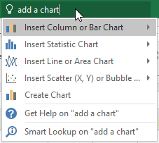
- To create a chart, click the Charts tab, then select a chart to visualize your data. Before you settle on a chart, just hover the cursor over each option to see a preview.
- To add quick chart data to individual cells, click the Sparklines tab and choose a format. Again, you can hover the cursor over each option to see a preview.
- To instantly apply conditional formatting (which is usually a little more complex in Excel) based on your data, use the Formatting tab. Here you can choose an option like Color or Data Bars, which apply colors to your data based on trends.


Advertisement
-
1
Quickly add data with AutoSum. AutoSum is a built-in Excel function that makes it easy to find the total of one or more columns in a few clicks. Functions or formulas that perform calculations and other tasks based on the values of cells. When you use a function to get something done, you’re creating a formula, which is like a math equation. If you have a column or row of numbers you want to add:
- Click the cell below the numbers you want to add (if a column) or to the right (if a row).[8]
- On the Home tab, click AutoSum toward the upper-right corner of the app. A formula beginning with =SUM(cell+cell) will appear in the field, and a dotted line will surround the numbers you’re adding.
- Press Enter or Return. You should now see the total of the numbers in the selected field. This is here because you created your first formula—which you didn’t have to write by hand!
- If you change any numbers in your data after using AutoSum, the AutoSum value will update automatically.
- Click the cell below the numbers you want to add (if a column) or to the right (if a row).[8]
-
2
Write a simple math formula. AutoSum is just the beginning—Excel is famous for its ability to do all sorts of simple and complex math calculations on data. Fortunately, you don’t have to be a math whiz to create simple formulas to create everyday math formulas, like adding, subtracting, and multiplying. Here’s some basic formulas to get you started:
-
Add: — Type =SUM(cell+cell) (e.g.,
=SUM(A3+B3)) to add two cells’ values together, or type =SUM(cell,cell,cell) (e.g.,=SUM(A2,B2,C2)) to add a series of cell values together.- If you want to add all of the numbers in a whole column (or in a section of a column), type =SUM(cell:cell) (e.g.,
=SUM(A1:A12)) into the cell you want to use to display the result.
- If you want to add all of the numbers in a whole column (or in a section of a column), type =SUM(cell:cell) (e.g.,
-
Subtract: Type =SUM(cell-cell) (e.g.,
=SUM(A3-B3)) to subtract one cell value from another cell’s value. -
Divide: Type =SUM(cell/cell) (e.g.,
=SUM(A6/C5)) to divide one cell’s value by another cell’s value. -
Multiply: Type =SUM(cell*cell) (e.g.,
=SUM(A2*A7)) to multiply two cell values together.
-
Add: — Type =SUM(cell+cell) (e.g.,


Advertisement
-
1
Select a cell for an advanced formula. What if you need to do something more complicated than just adding numbers? Even if you don’t know how to write formulas by hand, you can still create useful formulas that work with your data in various ways. Start by clicking the cell in which you want to display your formula.
-
2
Click the Formulas tab. It’s a tab at the top of the Excel window.
-
3
Explore the Function Library. Several function categories appear in the toolbar, such as Financial, Text, and Math & Trig. Click the options to check out the types of functions available, though they might not make a whole lot of sense just yet.
-
4
Click Insert Function. This option is in the far-left side of the Formulas toolbar. This opens the Insert Function window, which gives you a more detailed breakdown of each function.
-
5
Click a function to learn about it. You can type what you want to do (such as round), or choose a category to filter the list of functions. Then, click any function to read a description of how it works and view its syntax.
- For example, to select the formula for finding the tangent of an angle, you would scroll down and click the TAN option.
-
6
Select a function and click OK. This creates a formula based on the selected function.
-
7
Fill out the function’s formula. When prompted, type in the number or select a cell for which you want to use the formula.
- For example, if you select the TAN function, you’ll type in the number for which you want to find the tangent, or select the cell that contains that number.
- Depending on your selected function, you may need to click through a couple of on-screen prompts.
-
8
Press ↵ Enter or ⏎ Return to run the formula. Doing so applies your function and displays it in your selected cell.


Advertisement
-
1
Set up the chart’s data. If you’re creating a line graph or a bar graph, for example, you’ll want to use one column of cells for the horizontal axis and one column of cells for the vertical axis. The best way to do this is to place your data in a table.
- Typically speaking, the left column is used for the horizontal axis and the column immediately to the right of it represents the vertical axis.
-
2
Select the data in your table. Click and drag your mouse from the top-left cell of the data down to the bottom-right cell of the data.
-
3
Click the Insert tab. It’s a tab at the top of the Excel window.
-
4
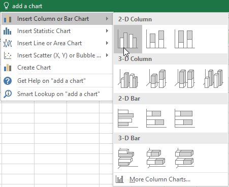
Click Recommended Charts. You’ll find this option in the «Charts» section of the Insert toolbar. A window with different chart templates will appear.
-
5
Select a chart template. Click the chart template you want to use based on the type of data you’re working with. If you don’t see a chart type you like, click the All Charts tab to explore by category, such as Pie, Bar, and X Y Scatter.
-
6
Click OK. It’s at the bottom of the window. This creates your chart.
-
7
Use the Chart Design tab to customize your chart. Any time you click your chart, the Chart Design tab will appear at the top of Excel. You can adjust the chart style here, change colors, and add additional elements.
-
8
Double-click a chart element to manage it in the Format panel. When you double-click something on your chart, such as a value, line, or bar, you’ll see options you can edit in the panel on the right side of excel. Here you can change the axis labels, alignment, and legend data.


Advertisement
Add New Question
-
Question
How do you add a check mark or an X mark to a cell?

You can go into Insert, then Symbol, and choose the symbol you want. After that, you can just copy and paste the symbol from one cell to another.
-
Question
Can I add work sheets on Excel?
Yes. At the bottom left of the Excel you will see the list of sheets. To the left of those sheets you will find a «+» sign. Click on it.
-
Question
How do I move cell contents to another cell?
Highlight the cell, right-click, and click Copy. Click destination cell, right-click and Paste.
See more answers
Ask a Question
200 characters left
Include your email address to get a message when this question is answered.
Submit
Advertisement
Video
Thanks for submitting a tip for review!
References
About This Article
Article SummaryX
1. Purchase and install Microsoft Office.
2. Enter data into individual cells.
3. Format cells based on certain criteria.
4. Organize data into rows and columns.
5. Perform math operations using formulas.
6. Use the Formulas tab to find additional formulas.
7. Use data to create charts.
8. Import data from other sources.
Did this summary help you?
Thanks to all authors for creating a page that has been read 646,263 times.
Reader Success Stories
-

«I am applying for a job that requires comprehensive knowledge of Excel. Well, I don’t have it, but this article…» more
Is this article up to date?
Lesson 1: Getting Started with Excel
Introduction
Excel is a spreadsheet program that allows you to store, organize, and analyze information. While you may think Excel is only used by certain people to process complicated data, anyone can learn how to take advantage of the program’s powerful features. Whether you’re keeping a budget, organizing a training log, or creating an invoice, Excel makes it easy to work with different types of data.
Watch the video below to learn more about Excel.
About this tutorial
The procedures in this tutorial will work for all recent versions of Microsoft Excel, including Excel 2019, Excel 2016, and Office 365. There may be some slight differences, but for the most part these versions are similar. However, if you’re using an earlier version, you may want to refer to one of our other Excel tutorials instead.
The Excel Start Screen
When you open Excel for the first time, the Excel Start Screen will appear. From here, you’ll be able to create a new workbook, choose a template, and access your recently edited workbooks.
- From the Excel Start Screen, locate and select Blank workbook to access the Excel interface.

The parts of the Excel window
Some parts of the Excel window (like the Ribbon and scroll bars) are standard in most other Microsoft programs. However, there are other features that are more specific to spreadsheets, such as the formula bar, name box, and worksheet tabs.
Click the buttons in the interactive below to become familiar with the parts of the Excel interface.
Working with the Excel environment
The Ribbon and Quick Access Toolbar are where you will find the commands to perform common tasks in Excel. The Backstage view gives you various options for saving, opening a file, printing, and sharing your document.
The Ribbon
Excel uses a tabbed Ribbon system instead of traditional menus. The Ribbon contains multiple tabs, each with several groups of commands. You will use these tabs to perform the most common tasks in Excel.
- Each tab will have one or more groups.
- Some groups will have an arrow you can click for more options.
- Click a tab to see more commands.
- You can adjust how the Ribbon is displayed with the Ribbon Display Options.
Certain programs, such as Adobe Acrobat Reader, may install additional tabs to the Ribbon. These tabs are called add-ins.
To change the Ribbon Display Options:
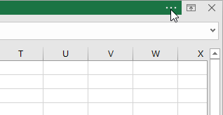
The Ribbon is designed to respond to your current task, but you can choose to minimize it if you find that it takes up too much screen space. Click the Ribbon Display Options arrow in the upper-right corner of the Ribbon to display the drop-down menu.
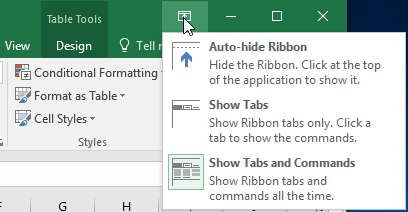
There are three modes in the Ribbon Display Options menu:
- Auto-hide Ribbon: Auto-hide displays your workbook in full-screen mode and completely hides the Ribbon. To show the Ribbon, click the Expand Ribbon command at the top of screen.
- Show Tabs: This option hides all command groups when they’re not in use, but tabs will remain visible. To show the Ribbon, simply click a tab.
- Show Tabs and Commands: This option maximizes the Ribbon. All of the tabs and commands will be visible. This option is selected by default when you open Excel for the first time.
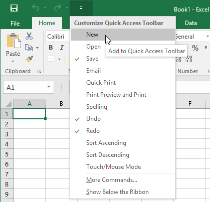
The Quick Access Toolbar
Located just above the Ribbon, the Quick Access Toolbar lets you access common commands no matter which tab is selected. By default, it includes the Save, Undo, and Repeat commands. You can add other commands depending on your preference.
To add commands to the Quick Access Toolbar:
- Click the drop-down arrow to the right of the Quick Access Toolbar.
- Select the command you want to add from the drop-down menu. To choose from additional commands, select More Commands.
- The command will be added to the Quick Access Toolbar.
How to use Tell me:
The Tell me box works like a search bar to help you quickly find tools or commands you want to use.
- Type in your own words what you want to do.
- The results will give you a few relevant options. To use one, click it like you would a command on the Ribbon.
Worksheet views
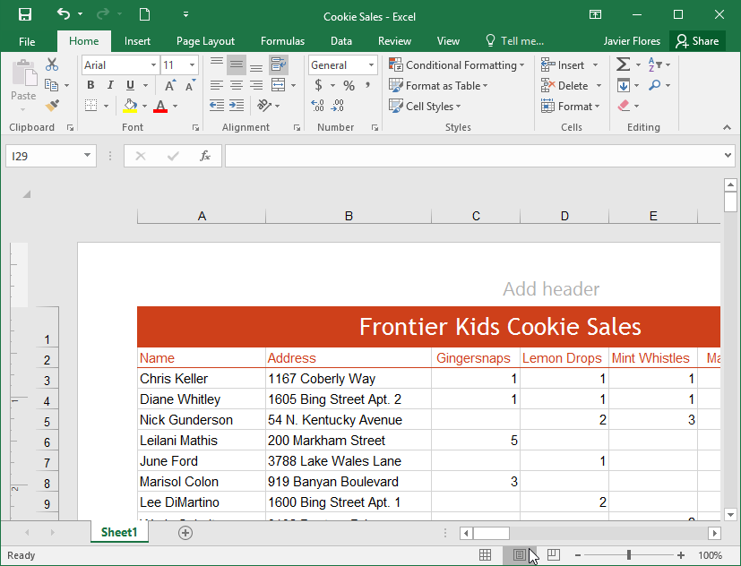
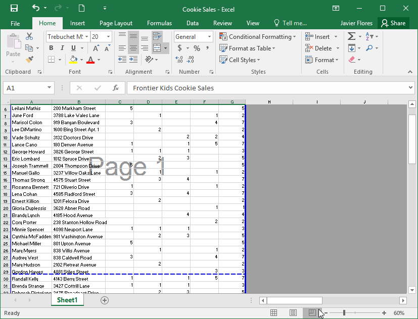
Excel has a variety of viewing options that change how your workbook is displayed. These views can be useful for various tasks, especially if you’re planning to print the spreadsheet. To change worksheet views, locate the commands in the bottom-right corner of the Excel window and select Normal view, Page Layout view, or Page Break view.
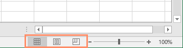
- Normal view is the default view for all worksheets in Excel.

- Page Layout view displays how your worksheets will appear when printed. You can also add headers and footers in this view.
- Page Break view allows you to change the location of page breaks, which is especially helpful when printing a lot of data from Excel.
Backstage view
Backstage view gives you various options for saving, opening a file, printing, and sharing your workbooks.
To access Backstage view:
- Click the File tab on the Ribbon. Backstage view will appear.
Click the buttons in the interactive below to learn more about using Backstage view.
Challenge!
- Open Excel.
- Click Blank Workbook to open a new spreadsheet.
- Change the Ribbon Display Options to Show Tabs.
- Using the Customize Quick Access Toolbar, click to add New, Quick Print, and Spelling.
- In the Tell me bar, type the word Color. Hover over Fill Color and choose yellow. This will fill a cell with the color yellow.
- Change the worksheet view to the Page Layout option.
- When you’re finished, your screen should look like this:
- Change the Ribbon Display Options back to Show Tabs and Commands.
- Close Excel and Don’t Save changes.
/en/excel/understanding-onedrive/content/
Launching the Excel Application
Upon starting the Excel application, you are presented with what is known as the Getting Started page.
This page serves as a branching off point to start or access many different types of Excel files. These include, but are not limited to:
- Starting a brand new blank workbook. This is where you begin when you are starting from zero.
- Starting a brand new workbook based on a template. Templates provide an existing framework with labels, formulas, and sample data. Templates are great if you are in a hurry or lack the needed skills to produce the needed output, such as Pivot Tables or Charts.
- Starting a file from the history list. This is a convenient way to open a file you have been working on in the recent hours or days without having to manually locate the file.
- Open a file not in the history. This is useful for files you may have downloaded from email attachments or recently gained access to via a USB device.

Starting a New, Blank Workbook
When you begin with a new, blank workbook, the workbook is not saved until you initially save the file.
To save the workbook, click the Save button in the Quick Access Toolbar (upper-left corner), provide a name and location to save the file, and click Save. You can also use the keyboard shortcut CTRL-S.

A single Excel file is often referred to as a workbook or spreadsheet. A workbook consists of at least one sheet.

Additional sheets can be added by clicking the “plus” button to the right of the sheet tabs.

You can rename a sheet by double-clicking on the sheet tab to enable rename mode.

The Layout of the Grid
Each sheet in a workbook is composed of a series of rows and columns. Where these rows and columns interest we have what are called cells.

Each sheet has the following dimensions:
- Columns = 16,384
- Rows = 1,048,576
- Cells = 17,179,869,184
This means you can place over 17 billion pieces of unique information on a single sheet.
Entering Data into a Cell
To enter information into a cell, click on the desired cell and start typing. If the cell began as an empty cell, the newly entered data will be displayed. If the cell contains information, that information will be replaced with the newly entered data.
Cell Addresses
Each of the over 17 billion cells on a sheet has a unique address. The address is a composite of the cell’s column position (a letter) and the cell’s row position (a number).

The Formula Bar
The Formula Bar is where formulas, numbers, or text can be edited after being placed in a cell.

Although you can edit the contents of a cell directly on the grid, this becomes more challenging when working with complex formulas or long passages of text. Performing the edits in the Formula Bar will prove a much easier task.
A cell containing numbers or text will display the same information on the Formula Bar as is displayed in the cell.
A cell that contains a formula will display the formula in the Formula Bar and the formula’s result in the cell.
The Name Box
The Name Box serves several purposes. One purpose is to display the address of the currently selected cell.

This will make it easier to accurately determine the address of the selected cell, especially if you happen to be zoomed out to a point where reading the row and column headings become difficult.
“Teleporting” to a Cell
When you need to position yourself in a cell that is a considerable distance from your current location, you can type the address of the destination cell into the Name Box and press Enter. This will instantly relocate you to the new cell.
Try the following cell address to see the end of the spreadsheet universe (lower-right corner of the sheet.)

To return to the “beginning” of the sheet (upper-left corner of the sheet) enter the cell address A1 into the Name Box and press Enter. You can also press the CTRL-Home keys to instantly relocate to cell A1.
Selecting Single/Multiple Rows & Columns
To select a row or column, click the applicable row or column header.

To select multiple rows or columns, click and hold the first row/column, then drag across the adjacent rows/columns until you have selected all the needed locations.
Shortcuts Galore
Excel has more shortcuts than probably anyone knows (at least anyone with a social life.)
One of the best shortcuts for selecting columns is CTRL-Space.

With the column selected, holding the Shift key while repeatedly pressing the left/right arrow keys will select multiple adjacent columns.
NOTE: If you want to see a demonstration of many of the most popular Excel keyboard shortcuts, check out this post and video:
Useful Excel Shortcuts
When you right-click a cell, you will receive a menu of options. The options displayed are directly related to the object you have right-clicked on.

With selected columns or rows, clicking the Insert or Delete options in the right-click menu will either add or remove columns or rows in the same quantity selected.
Coolest Way to Add/Remove Rows & Columns
When you select a row or column, or a series of rows or columns, you can press the CTRL-plus or CTRL-minus keys to quickly add or delete rows or columns.
It is likely to be easier to perform this using the plus/minus keys on the numeric keypad. If you use the plus/minus button located above the letter keys, you will have to add the extra step of using Shift when using the plus key.
Moving to the Extents of the Sheet or Data
You can use the CTRL key along with the up/down/left/right arrow keys to navigate to the extent of the sheet, or if you have existing data, the extent of the data range.

Defining Ranges of Cells
An important term to understand is the word Range. A Range is either a single cell or a group of cells.
When we define a range in a formula, we always refer to the range starting from the upper-left corner of the range to the lower-right corner of the range. We place a colon between the two range addresses to symbolize the word “through”.
Selecting and Moving Cells
When you move your pointer around the grid, you will see a large white plus symbol known as the General Select symbol.

Placing this symbol in the center of a cell and clicking will select the designated cell.
If you place your General Select symbol in the green edge of the selected cell, you will see the large, white plus change to a thinner, black directional arrow known as the Move icon.

If you click and drag from the green border, you will move the selected cell or range of cells.
If you need to move data between sheets, workbooks, or great distances on the same sheet, you can use the traditional Cut-Paste technique.
The Fill Series Handle
One of the greatest data entry time-savers is the Fill Series handle.

When you place your pointer over this green handle, your large, white plus symbol will change to a thin, black plus symbol.

When you see this symbol, click and drag it down or to the right to invoke the Fill Series feature.
Below is a shortlist of things the Fill Series feature will perform:
- Repeat text
- Create lists of months
- Create a list of weekday names
- Create lists of days
- Repeat formulas
- Repeat cell formatting

Resizing Rows and Columns
If you require more width for your columns (typically for text entries), you can hover your pointer over the right column divider (i.e., the divider between columns D & E to resize column D) and click to drag the divider left or right as needed.

You can perform the same operation on rows by selecting the bottom divider for a specific row and drag up and down as needed.
If you place your pointer over a column or row divider and double-click the mouse, you can invoke an “Auto-Fit” command. This will enlarge or shrink the row/column to the optimal size based on the data contained on that row or column.
Wrapping Text within a Cell
If you don’t want to have an overly wide column to accommodate the contained text, you can activate the Wrap Text feature to have the text automatically apply in-cell carriage returns based on the data and the size of the cell.

You can remove this feature by selecting the wrapped text cell and clicking the Wrap Text button to toggle the feature to the off state.
Touring the Ribbon
The Tabs and the Ribbon provide access to many of the program’s features.

Clicking the various Tabs will reveal collections of similarly purposed features.
Most of the structural changes made to sheets, like paper size, margin sizes, paper orientation are found on the Page Layout ribbon.

The most used features of the program are located on the Home tab/ribbon.
Learning About Buttons
If you are unsure as to what a particular button will do for you, you can hover your pointer over the button to reveal the “Tell me more” information.

This provides a brief explanation of the button’s purpose, its keyboard shortcut key sequence (if applicable), and a link to open the official Microsoft documentation page for the feature.
Accessing the “Deep Dive” Features
Many of the Ribbon groupings have more features than can be displayed without making the Ribbon overly complicated. For these lesser-used features, you can click the “additional options” button located in the lower-right corner of the button group.

These will open various dialog boxes that contain additional features related to the button group’s overall purpose.
Giving More Space to the Grid
If you want to give more screen space to the grid (and less to the Ribbon), you can either click the “Collapse the Ribbon” button (upper-right corner) or press the CTRL-F1 key combination.

The Ribbon will be hidden leaving only the Tabs visible.

The Ribbon is still accessible by clicking a Tab, but it will automatically hide once it has served its purpose.
NOTE: You can also double-click a Tab to apply or remove this auto-hide behavior of the Ribbon. Many users “discover” this feature accidentally by double-clicking a Tab and thinking they have just lost their Ribbon. Not to worry; double-clicking a Tab will remedy the situation.
Accessing the Backstage
Clicking the File tab will reveal the Backstage.


The Backstage is where you go to manipulate the file as an object.
What I mean is you are trying to perform actions such as:
- Save the file
- Open a file
- Close a file
- Print a file
- Email the file
- Convert the file (ex: PDF, or delimited text)
- Protect the file (e., password to open or password to edit)
- Obtain file statistics (ex: size, author, creation date, last saved date, etc.)
Shortcuts for Inputting Values
Getting Out of Edit Mode
When entering data, pressing the Tab key will move the cursor right to the next column, while pressing Enter will move the cursor down to the next row.
If you wish to enter the data without relocating the cursor, press CTRL-Enter.
Getting Into Edit Mode
If you need to edit the contents of a cell, you can select the cell and then press the F2 key. This will enable Edit Mode and place your cursor at the end of the cell’s contents.
Repeating Cell Data
If you have text, numbers, or formulas in a cell, select the cell and adjoining cells to the left or below then press either CTRL-R or CTRL-D to repeat the first cell’s contents to the other selected cells either to the right on the row or downward (below) in the column.
Confining the Data Entry Cells
If you know you wish to restrict the data to a set range of rows and columns, you can pre-select the range. By doing so, repeated pressing of the Tab key will confine the cell selections to the pre-selected range.

Formatting Data (Let’s make this pretty!)
We have a set of data where department headcounts are displayed by month.

Attractive Titles
To make the report more attractive, we begin by centering the heading between columns A and G. This is accomplished by selecting the cells you wish to center across (A1 through G1) and press the Merged & Center button.

Resizing Multiple Columns
If you wish to tighten up the space used by the monthly columns (B through G), select the column headings for columns B through G, then double-click one of the highlighted column heading dividers (remember Auto Fit?).

If this is too tight, you can manually expand one of the selected column heading dividers and manually resize to the desired width. This new size will be applied to all selected columns, providing a professional, uniformed look.
Adding Colors and Borders
With the Month cells selected, we can apply any traditional cosmetic changes to the cells, like font style, font size, font color, alignment, etc.
We can also add borders and fill colors to the cells using the Borders and Fill Color features.

Moving Rows (the COOL Way)
Suppose you want to move the order of the Departments in our table above.
Most users would perform the following steps:
- Insert a blank row where they want the data to be moved to
- Select the data to be moved
- Invoke a Cut action
- Select the newly inserted empty row
- Invoke a Paste action (or right-click -> “Insert Cut Cells”)
Although that works, it’s not exactly a crowd-pleasing party trick. Try this instead:
- Select the cells you wish to relocate (ex: A7 through G7).
- Click and hold the border of the highlighted cells (stay away from the Fill Series handle).
- While you drag up or down, press the SHIFT This will reveal a thick green line that indicates the drop location.

Speedy Formatting Trick
If you have a cell that has a certain style (i.e., color, size, font, etc.) and you want all of those same settings applied to other cells, you can use the Format Painter to copy and paste the look of a cell without carrying over the data.

Select the cell that has the style you wish to replicate, click the Format Painter button, then click the cell to which you want to apply the style.
Pro Tip: If you need to apply the style to many cells that may not be in a consecutive arrangement, double-click the Format Painter button to lock it into an “on” state. Select all the needed cells, then click the Format Painter when you’re finished to deactivate the feature or press the ESC key.
Creating Your First Calculations (Adding Values)
If we want to get the monthly totals for all Departments, select the cell below the “Jan” values (cell B8) and press the AutoSum button (or press the ALT-Equals sign) located in the upper-right corner of the Home ribbon.

This will create a formula that uses the SUM function. The formula will attempt to determine the extent of the data. We can easily verify the selection by examining the Marquee (moving dotted line surrounding the selected cells).

Repeating Formulas
If you need to create the same type of formulas for the remaining months, perform the following steps:
- Select the cell with the formula you wish to repeat.
- Place the mouse pointer (thick, white plus symbol) over the Fill Series You should see a thin, black plus symbol.
- Drag the Fill Series handle to the right across the remaining columns of calculations.


Closing Thoughts
Knowing a few of the most used features of Excel will give you the confidence to want to learn more.
The journey to learn Excel is endless, but as with all journeys, it must begin with a few small steps.
Today you walk, tomorrow you run, and soon you will fly.
Published on: February 5, 2021
Last modified: March 24, 2023


Leila Gharani
I’m a 5x Microsoft MVP with over 15 years of experience implementing and professionals on Management Information Systems of different sizes and nature.
My background is Masters in Economics, Economist, Consultant, Oracle HFM Accounting Systems Expert, SAP BW Project Manager. My passion is teaching, experimenting and sharing. I am also addicted to learning and enjoy taking online courses on a variety of topics.