How to split a column in excel

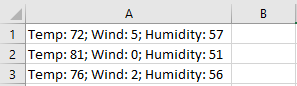
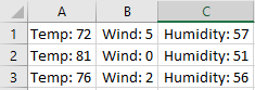
You might want to split a cell into two smaller cells within a single column. Unfortunately, you can’t do this in Excel. Instead, create a new column next to the column that has the cell you want to split and then split the cell. You can also split the contents of a cell into multiple adjacent cells.

See the following screenshots for an example:

Split the content from one cell into two or more cells

1. Select the cell or cells whose contents you want to split.

   Important: When you split the contents, they will overwrite the contents in the next cell to the right, so make sure to have empty space there.

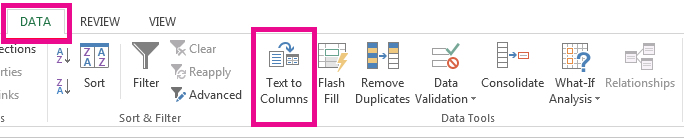
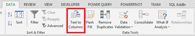
2. On the Data tab, in the Data Tools group, click Text to Columns. The Convert Text to Columns Wizard opens.

   

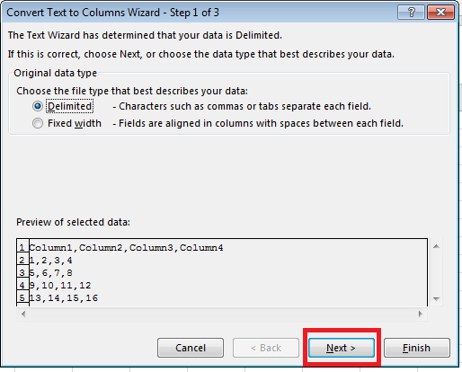
3. Choose Delimited if it is not already selected, and then click Next.

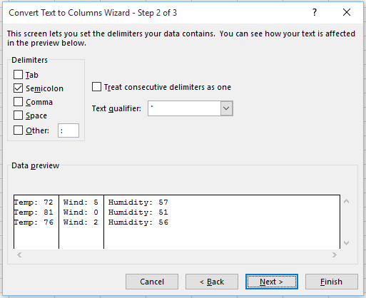
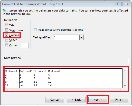
4. Select the delimiter or delimiters to define the places where you want to split the cell content. The Data preview section shows you what your content would look like. Click Next.

   

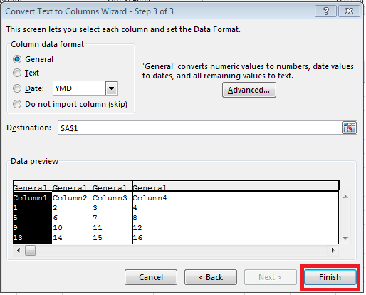
5. In the Column data format area, select the data format for the new columns. By default, the columns have the same data format as the original cell. Click Finish.

See Also

Merge and unmerge cells

Merging and splitting cells or data

Do you have any tricks on how to split columns in excel? When working with Excel, you may need to split grouped data into multiple columns. For instance, you might need to separate the first and last names into separate columns. 

With Excel’s “Text to Feature” there are two simple ways of splitting your columns. If there is an evident delimiter such as a comma, use the “Delimited” option. However, the “Fixed method is ideal for splitting the columns manually.”

To learn how to split a column in excel and make your worksheet easy-to-read, follow these simple steps. You can also check our Microsoft Office Excel Cheat Sheet here. But, first, why should you split columns in excel? 

Jump to:

• Why you need to split cells
• How do you split a column in excel?
• Method 1- Delimited Option
• Method 2- Fixed Width
• How to Split One Column into Multiple Columns in Excel
• Method 3- Split Columns by Flash Fill
• Method 4- Use LEFT, MID and RIGHT text string functions 

Why you need to split cells

If you downloaded a file that Excel can’t divide, then you need to separate your columns. You should split a column in excel if you want to divide it with a specific character. Some examples of familiar characters are commas, colons, and semicolons.

How do you split a column in excel?

Method 1- Delimited Option

This option works best if your data contains characters such as commas or tabs. Excel only splits data when it senses specific characters such as commas, tabs, or spaces. If you have a Name column, you can separate it into First and Last name columns

1. First, open the spreadsheet that you want to split a column in excel
2. Next, highlight the cells to be divided. Hold the SHIFT key and click the last cell on the range
3. Alternatively, right-click and drag your mouse to highlight the cells
4. Now, click the Data tab on your spreadsheet.
5. Navigate to and click on the “Text to Columns” From the Convert Text to Columns Wizard dialog box, select Delimited and click “Next.”
6. Choose your preferred delimiter from the options given and click “Next.”
7. Now, highlight General as your Column Data Format
8. “General” format converts all your numeric values to numbers. Date values are converted to dates, and the rest of the data is converted to text. “Text” format only converts the data into text. “Date” allows you to select your desired date format. You can skip the column by choosing “Do not import column.” 
9. Afterward, type the “Destination” field for your new column. Otherwise, Excel will replace the initial data with the divided data
10. Click “Finish” to split your cells into two separate columns.

Method 2- Fixed Width 

This option is ideal if spaces separate your column data fields. So, Excel splits your data based on the character counts, be it 5th or 10th characters.  

1. Open your spreadsheet and select the column you wish to split. Otherwise, the “Text Columns” will be inactive. 
2. Next, click Text Columns in the “Data” Tab
3. Click Fixed Width and then Next
4. Now you can adjust your column breaks in the “Data preview.” Unlike the “Delimited” option that focuses on characters, in “Fixed Width,” you select the position of splitting the text.
5. Tips: Click the preferred position to CREATE a line break. Double-Click on the line to delete it. Click and drag a column break to move it
6. Click Next if you’re satisfied with the results
7. Select your preferred Column Data Format 
8. Next, type the “Destination” field for your new column. Otherwise, Excel will replace the initial data with the divided data.
9. Finally, click Finish to confirm the changes and divide your column into two

How to Split One Column into Multiple Columns in Excel

A single column can be split into multiple columns using the same steps outlined in this guide

Tip: The number of columns depends on the number of delimiters that you select. For instance, Data will be split into three columns if it contains three commas.

Method 3- Split Columns by Flash Fill

If you are using Excel 2013 and 2016, you are in luck. These versions are integrated with a Flash fill feature that extracts data automatically once it recognizes a pattern. You can use flash fill to split the first and last name in your column. Alternatively, this feature combines separate columns into one column.

If you don’t have these professional versions, quickly upgrade your Excel version. Follow these steps to divide your columns using Flash Fill. 

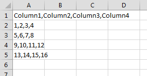
• Assume your data resembles the one in the image below

• Next, in cell B2, type the First Name as below

• Navigate to the Data Tab and click Flash Fill. Alternatively, use the shortcut CTRL+E
• Selecting this option automatically separates all the First Names from the given column

Tip: Before clicking Flash Fill, ensure that cell B2 is selected. Otherwise, a warning appears that

• Flash Fill cannot recognize a pattern to extract the values. Your extracted values will look like this: 

 

• Apply the same steps for the last name as well.

 

Now, you have learned to split a column in excel into multiple cells 

Method 4- Use LEFT, MID and RIGHT text string functions 

Alternatively, use LEFT, MID, and RIGHT string functions to split your columns in Excel 2010, 2013 and 2016. 

• LEFT function: Returns the first character or characters on your left, depending on the specific number of characters you require.
• MID Function: Returns the middle number of characters from string text beginning from where you specify.
• RIGHT Function: Gives the last character or characters from your text field, depending on the specified number of characters on your right.

However, this option is not valid if your data contains a formula such as VLOOKUP. In this example, you’ll learn how to split Address, City, and zip code columns.

 

To extract the Addresses using the LEFT function:

1. First select cell B2
2. Next, apply the formula =LEFT(A2,4)

Tip: 4 represents the number of characters representing the address

    3. Click, hold and drag down the cell to copy the formula to the entire column

To extract the City data, use the MID function as follows:

• First, Select cell C2
• Now, apply the formula =MID(A2,5,2)

Tip: 5 represents the fifth character. 2 is the number of characters representing the city.

• Right-click and drag down the cell to copy the formula in the rest of the column

Finally, to extract the last characters in your data, use the Right text function as follows:

• Select Cell D2
• Next, apply the formula =RIGHT(A2,5)

Tip: 5 represents the number of characters representing the Zip Code

• Click, hold and drag down the cell to copy the formula in the entire column

Tips to remember

• The shortcut key for Flash Fill is CTRL+E
• Always try to identify a shared value in your column before splitting it
• Familiar characters when splitting columns include commas, tabs, semicolons, and spaces. 

Text Columns is the best feature to split a column in excel. It might take you several attempts to master the process. But once you get the hang of it, it will only take you a couple of seconds to split your columns. The results are professional, clean, and eye-catching columns. 

 If you’re looking for a software company you can trust for its integrity and honest business practices, look no further than SoftwareKeep. We are a Microsoft Certified Partner and a BBB Accredited Business that cares about bringing our customers a reliable, satisfying experience on the software products they need.   We will be with you before, during, and after all the sales.

The easiest way on how to split Cells in Excel or split Columns in Excel, is to select the column you want to split. Next go to the Data ribbon and hover to the Data Tools group. Next Select Text to Columns and proceed according to the instructions.

The above works for simple splits on delimiters such as Commas, Semicolons, Tabs etc. However, for Non-Standard patterns such as Capital letters, specific word you might need to revert to more elaborate solutions such using VBA String functions or the VBA Regex. Read on to learn more.

Splitting Cells using Text to Columns

A Delimiter is a sequence of 1 or more characters to separate columns within a Text String. An example of a Delimiter is the Comma in the following Text String Columns1,Column2 which separates the String Column1 from Column2. Popular Delimiters often used are: Commas (,), Semicolons (;), Dots (.), Tabs (t), Spaces (s). A Delimiter can be just as well any Sequence of Characters.

How to Split Cells in Excel using Text to Columns

The most obvious choice when wanting to Split Cells in Excel is to use the DATA Ribbon Text to Columns feature.

Select the Column

Select the Column with Cells you want to Split in Excel:

Select first column and proceed to Text to Columns

Select the entire first column where all your data should be located. Next click on the Text to Columns button in the DATA ribbon tab:

Proceed according to Wizard instructions

This is the hard part. Text to Columns need additional information on the delimiter and format of your columns.

Delimited or Fixed width?

Delimiters are any specific Sequence of Characters (like a comma or semicolon). Fixed Width means that each column in the Cell is separated by a Fixed Width of Whitespace Characters. In this case we select Delimited. Next click Next to proceed.

Select delimiter

Assuming your columns are separated with a specific Delimiter you need to provide this delimiter in the Wizard. Look at the Data preview to make sure your columns will be separated correctly. When finished proceed with Next

Format your columns (optional)

The last step is to format your columns if needed. If your columns represent Dates or you want to pull a column containing numbers/dates as text instead – be sure to format it appropriately. Usually, however, you are fine with hitting Finish:

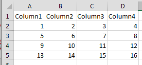
The Resulting Split Columns

If you have proceeded according to the steps above you should have a neatly formatted spreadsheet like the one below.

Splitting Cells using Formulas

Another way of how to Split Cells in Excel is using the LEFT, RIGHT and LEN functions. See examples below:

Splitting against a Delimiter:

'Cell A1
Hello;There

The formula:

'To get "Hello"
=LEFT(A1;FIND(";")-1)

'To get "There"
=RIGHT(A1;LEN(A1)-FIND(";"))

Split Cells on Patterns

Sometimes instead of Delimiters you want to Split your Excel Cells on Patterns that are dynamic and may be different for each cell in a certain column. Fortunately Excel supports Regular Expressions, which allow you to Define Patterns on which your Cells are to be Split.

Let us first introduce my often used GetRegex UDF function:

'str - the original string. reg - the Regex pattern. index - the index of the capture if more than 1.
Public Function GetRegex(str As String, reg As String, Optional index As Integer) As String
    On Error Resume Next
    Set regex = CreateObject("VBScript.RegExp")
    regex.Pattern = reg
    regex.Global = True
    If index < 0 Then index = 0
    If regex.test(str) Then
        Set matches = regex.Execute(str)
        GetRegex = matches(index).SubMatches(0)
        Exit Function
    End If
    GetRegex = ""
End Function

To install it – open your DEVELOPER Excel Tab, click Visual Basic and add the code above to any new VBA Module.

If you are not familiar with Regular Expressions read the VBA Regex Tutorial.

What does this UDF function do? It extracts any text that matches a certain pattern. Let’s see it in action:

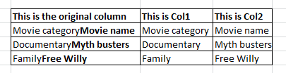
Example 1: Splitting Cells on Capital Letters

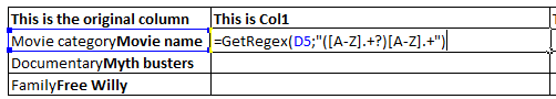
Let us take a common example where we have 1 Column of Cells that have 2 merged Columns inside. We want to split them on the second capital letter:

Now splitting this on the second capital letter using the FIND, LEFT, RIGHT and LEN functions will be a nightmare.

Let’s decipher the regular expression now:

Pattern	Description
[A-Z].+?	This will catch all words and whitespaces starting with a Capital letter the ? sign means that this is a non-greedy regular expression
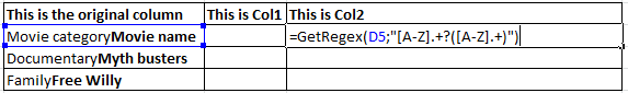
([A-Z].+?)	The () brackets will capture inside any pattern matching this regular expression
([A-Z].+?)[A-Z].+	The final regex this will capture only the first words and whitespaces starting with a Capital letter. Notice that the capture will end at the next Capital letter

Now for the second column:

Great right? Now just drag the formula across the rows – and you are done!

Example 2: Splitting Cells on Whitespaces

A simple example – let us Split an Excel Cell on a Variable number of Whitespace characters. Let us say the Words in our String can have 1 or more Spaces in between.

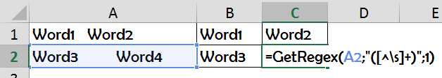
The Formula for the above is:

=GetRegex(A1;"s*?([^s]+)s*?";0)

Again let us break it down:

Pattern	Description
[^s]	This specifies a non-whitespace character
[^s]+	This specifies at least 1 non-whitespace character
([^s]+)	The () brackets will capture inside any pattern matching this regular expression – hence all sequences of non-whitespace characters

Split Excel Function

If you just need an Excel Split function and you can introduce the following UDF Function (copy to VBA Module):

Public Function SplitFunction(str As String, delimiter As String, index As Long) As String
    SplitFunction = Split(str, delimiter)(index)
End Function

It uses the VBA Split function which is available in VBA only.

Parameters

str
A String.

delimiter
The delimiter on which the Split operation is to be done.

index
The index of the substring resulting from the Split.

How to use the Excel Split Function

The Function will be available as an Excel Function:

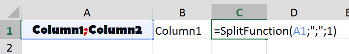
The above Formula looks like this (return second substring from Split):

=SplitFunction(A1;";";1)

There can be situations when you have to split cells in Excel. These could be when you get the data from a database or you copy it from the internet or get it from a colleague.

A simple example where you need to split cells in Excel is when you have full names and you want to split these into first name and last name.

Or you get address’ and you want to split the address so that you can analyze the cities or the pin code separately.

How to Split Cells in Excel

In this tutorial, you’ll learn how to split cells in Excel using the following techniques:

• Using the Text to Columns feature.
• Using Excel Text Functions.
• Using Flash Fill (available in 2013 and 2016).

Let’s begin!

Split Cells in Excel Using Text to Column

Below I have a list of names of some of my favorite fictional characters and I want to split these names into separate cells.:

Here are the steps to split these names into the first name and the last name:

• Select the cells in which you have the text that you want to split (in this case A2:A7).
• Click on the Data tab
• In the ‘Data Tools’ group, click on ‘Text to Columns’.
• In the Convert Text to Columns Wizard:

This will instantly split the cell’s text into two different columns.

Note:

• Text to Column feature splits the content of the cells based on the delimiter. While this works well if you want to separate the first name and the last name, in the case of first, middle, and last name it will split it into three parts.
• The result you get from using the Text to Column feature is static. This means that if there are any changes in the original data, you’ll have to repeat the process to get updated results.

Split Cells in Excel Using Text Functions

Excel Text functions are great when you want to slice and dice text strings.

While the Text to Column feature gives a static result, the result that you get from using functions is dynamic and would automatically update when you change the original data.

Splitting Names that have a First Name and Last Name

Suppose you have the same data as shown below:

Extracting the First Name

To get the first name from this list, use the following formula:

=LEFT(A2,SEARCH(" ",A2)-1)

This formula would spot the first space character and then return all the text before that space character:

This formula uses the SEARCH function to get the position of the space character. In the case of Bruce Wayne, the space character is in the 6th position. It then extracts all the characters to the left of it by using the LEFT function.

Extracting the Last Name

Similarly, to get the last name, use the following formula:

=RIGHT(A2,LEN(A2)-SEARCH(" ",A2))

This formula uses the search function to find the position of the spacebar using the SEARCH function. It then subtracts that number from the total length of the name (that is given by the LEN function). This gives the number of characters in the last name.

This last name is then extracted by using the RIGHT function.

Note: These functions may not work well if you have leading, trailing or double spaces in the names. Click here to learn how to remove leading/trailing/double spaces in Excel.

Splitting Names that have a First Name, Middle Name, and Last Name

There may be cases when you get a combination of names where some names have a middle name as well.

The formula in such cases is a bit complex.

Extracting the First Name

To get the first name:

=LEFT(A2,SEARCH(" ",A2)-1)

This is the same formula we used when there was no middle name. It simply looks for the first space character and returns all the characters before the space.

Extracting the Middle Name

To get the Middle Name:

=IFERROR(MID(A2,SEARCH(" ",A2)+1,SEARCH(" ",A2,SEARCH(" ",A2)+1)-SEARCH(" ",A2)),"")

MID function starts from the first space character and extracts the middle name by using the difference of the position of the first and the second space character.

In cases there is no middle name, the MID function returns an error. To avoid the error, it is wrapped within the IFERROR function.

Extracting the Last Name

To get the Last Name, use the below formula:

=IF(LEN(A2)-LEN(SUBSTITUTE(A2," ",""))=1,RIGHT(A2,LEN(A2)-SEARCH(" ",A2)),RIGHT(A2,LEN(A2)-SEARCH(" ",A2,SEARCH(" ",A2)+1)))

This formula checks whether there is a middle name or not (by counting the number of space characters). If there is only 1 space character, it simply returns all the text to the right of the space character.

But if there are 2, then it spots the second space character and returns the number of characters after the second space.

Note: These formula works well when you have names that have either the fist name and last name only, or the first, middle, and last name. However, if you have a mix where you have suffixes or salutations, then you’ll have to modify the formulas further.

Split Cells in Excel Using Flash Fill

Flash Fill is a new feature introduced in Excel 2013.

It could be really handy when you have a pattern and you want to quickly extract a part of it.

For example, let’s take the first name and the last name data:

Flash fill works by identifying patterns and replicating it for all the other cells.

Here is how you can extract the first name from the list using Flash Fill:

How Flash Fill Works?

Flash Fill looks for the patterns in the data set and replicates the pattern.

Flash Fill is a surprisingly smart feature and works as expected in most of the cases. But it also fails in some cases too.

For example, if I have a list of names that has a combination of names with some having a middle name and some don’t.

If I extract the middle name in such a case, Flash Fill will erroneously return the last name in case there is no first name.

To be honest, that’s still a good approximation of the trend. However, it is not what I wanted.

But it still is a good enough tool to keep in your arsenal and use whenever the need arises.

Here is another example where Flash Fill works brilliantly.

I have a set of addresses from which I want to quickly extract the city.

To quickly get the city, enter the city name for the first address  (enter London in cell B2 in this example) and use the autofill to fill all the cells. Now use Flash Fill and will instantly give you the name of the city from each address.

Similarly, you can split the address and extract any part of the address.

Note that this would need the address to be a homogenous data set with the same delimiter (comma in this case).

In case you try and use Flash Fill when there is no pattern, it will show you an error as shown below:

In this tutorial, I have covered three different ways to split cells in Excel into multiple columns (using Text to Columns, formulas, and Flash Fill)

Hope you found this Excel tutorial useful.

You May Also Like the Following Excel Tutorials:

• How to Quickly Combine Cells in Excel.
• How to Extract a Substring in Excel Using Formulas.
• How to Count Cells that Contain Text Strings.
• Extract Usernames from Email Ids in Excel [2 Methods].
• How to Split Multiple Lines in a Cell into Separate Cells/Columns.

When working with data and spreadsheets, readability, and structure matter a lot.

It makes the data easier to skim through and work with. One of the best ways to make your data more readable is to split it into chunks so that it is easier to access the right information.

When entering data from scratch, it’s possible to ensure that we structure the data to be more readable. However, sometimes you need to work with data that someone else has created.

If the volume of the data is very large then it’s usually quite difficult to structure the data’s readability.

For example, you might have got data with a list of names, and you might want to arrange the names in alphabetical order of surnames.

In other cases, you might have got a list of addresses, but want to organize this data properly so you can clearly see how many of the people reside in, say, New York.

The best way to work through the above two problems is by splitting one column into multiple columns.

The new versions of Excel provide a special feature that lets you do that using the ‘Data’ menu.

Let’s see how this can be achieved in both the above cases.

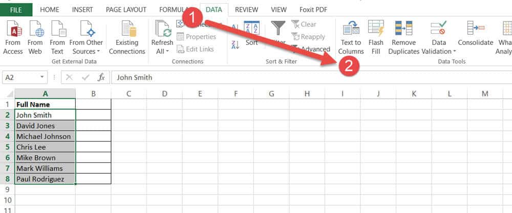
Say you have a list of names that you want to split into columns Name and Surname.

1. Select the column that you want to split
2. From the Data ribbon, select “Text to Columns” (in the Data Tools group). This will open the Convert Text to Columns wizard.
3. Here you’ll see an option that allows you to set how you want the data in the selected cells to be delimited. Make sure this option is selected. If you’re not familiar with the term ‘delimited’, it is the character that specifies how the data in the cells are separated from each other, for example, the first name and last name in each cell are separated by a space. This means the delimiter here is a space character.
4. Click Next
5. Here are the settings you need to do in the second steps of the Tetx to Columns wizard:
   • By default, you’ll find the Tab delimiter checked. But we don’t want to use that. We want to use Space delimiter. So uncheck the Tab delimiter and check the Space option (1).
   • There is also a checkbox that lets you specify if you want to treat consecutive delimiters as one(2). That means if you have two spaces between names by mistake, do you want to treat it as one space?
   • You can see how your data is going to look after the split in the data preview area (3) at the bottom of the dialog box. Notice when the space option is checked we get exactly the result we want.
   • Finally Click Next (4)
6. You’ll now see an option where you can specify the format for the data in the columns. By default, the General option is selected, which ensures that the columns have the same format as the original cells. Leave it with the General option selected and then click Finish.

We now have two columns of data, with the first name in Column A and last name in Column B.

It’s important to note that when you split the contents of a cell, Excel does not insert new cells to hold the contents.

So the new cells will overwrite the contents in the next cell on the right. Therefore, you should make sure that you leave an empty space on the right before splitting.

You also have the option to select the destination of the split data.

You can specify this during Step 7 by typing in the location where you want the split cells to be displayed in the destination input box. You can also select the destination cell from here.

It goes without saying that the number of columns that your data will be split into depends on the delimiters that you selected.

That means if you have a comma as a delimiter and in some cells, you have three words separated by commas then your data will be split into three columns.

How to Split Multiple Lines in a Cell into Multiple Cells

Now let’s discuss how to go about cases where you have a lot of information provided in separate lines of a cell.

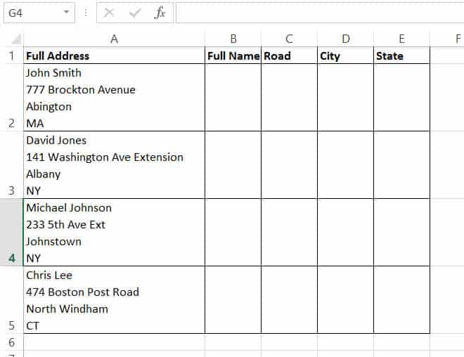
Take for example the sheet below.

Here you can see a whole address given in each cell. Each part of the address is on a separate line of a cell. Separating this column into four different columns that can show the full name of the person, Street, City and Country would make it much easier to identify patterns in the data.

Unfortunately separating cells with multiple lines is not as easy as the method given above. But it’s not too tough either. Here’s how you can go about this problem.

1. Select the column that you want to split
2. From the Data ribbon, select “Text to Columns” (in the Data Tools group). This will open the Convert Text to Columns wizard.
3. Here you’ll see an option that allows you to set how you want the data in the selected cells to be delimited. Make sure this option is selected.
4. Click Next
5. By default, you’ll find the Tab delimiter checked. Uncheck all the checked delimiters and select the ‘Other’ option. In the small box next to this option, you need to specify the delimiter character that you want to use. If you want to specify a line break character. Press Ctrl + J on your keyboard. This will show a tiny blinking dot inside the box. This means that the line break delimiter has been inserted.

You can see how your data is going to look after the split in the data preview area at the bottom of the dialog box.

Notice we get exactly the result we want. We have all the names in the first column, the second lines (Street names) in the second column, the city names in the third column, and the country names in the fourth column.

1. Click Next.
2. You’ll now see an option where you can specify the format for the data in the columns. By default, the General option is selected, which ensures that the columns have the same format as the original cells.
3. Here we also want all the columns to appear from column B onwards so the new cells don’t overwrite the existing column. Next to Destination, we see the cell ‘$A$2’ written. We can change this by selecting our required destination cell ‘$B$2’ and then click Finish.
4. You might get a dialog box asking you if you want to replace the data that is already present in the destination cells. Click on OK.

Once this is done, you will find columns B through E each containing a separate element of the address that was present in Column A.

How to Split up a Merged Cell

Before we end the article we want to add one more case. You may have more than one cells merged together and be looking for a way to unmerge or split these cells. We would like to also address this issue, in case you landed on our page looking for a solution to that. Here are the steps:

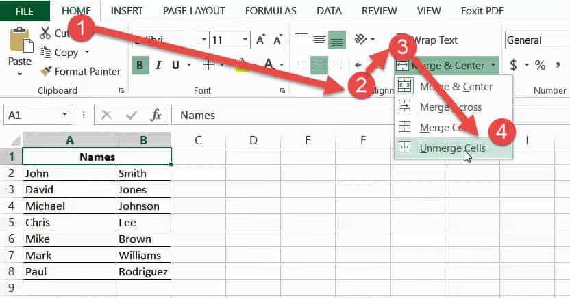
1. Click on the merged cell. If there is more than one cell that you want to un-merge, select all of them.
2. Under the Home Tab’s Alignment tools, you will see a drop-down next to the option that says Merge and Center. Click on the dropdown arrow and select “Unmerge Cells”.
3. This will split the merged cell back to the original number of cells.

Note that Excel does not have the option to split an unmerged cell into smaller cells (as is possible in MS Word).

We have discussed how you can split cells in Excel into separate cells using different types of delimiters. We have also taken a brief look at how to split cells that had been previously merged.

The above steps have been specified assuming that you are using Excel versions 2013 to 2019. However, Microsoft keeps updating its menus, tabs, and options in every new version it brings out.

So we cannot say for sure if the methods we mentioned will work on later versions of Excel.

I hope you found this tutorial useful!

Other Excel tutorials you may find useful:

• How to Find Merged Cells in Excel
• How to Merge First and Last Name in Excel
• How to Make all Cells the Same Size in Excel (AutoFit Rows/Columns)
• How to Remove Apostrophe in Excel
• How to Remove Commas in Excel (from Numbers or Text String)
• How to Flip Data in Excel (Columns, Rows, Tables)?
• How to Convert Columns to Rows in Excel?
• How to Combine Two Columns in Excel (with Space/Comma)