How to set up excel - Word и Excel - помощь в работе с программами

The best way to learn about Excel 2013 is to start using it. Create a blank workbook and learn the basics of working with columns, cells, and data.

Start using Excel

The best way to learn about Excel 2013 is to start using it.
You can open an existing workbook, or start with a template. Then, add some data into cells, use the ribbon, use the mini toolbar.

Want more?

What’s new in Excel 2013

Basic tasks in Excel

The best way to learn about Excel 2013 is to start using it.

This is what you see when you start Excel for the first time.

You can open an existing workbook over here or start with a template.

Since this is our first time, let’s keep it simple and select Blank workbook.

The area down here is where you create your worksheet.

And you’ll find all the tools you need to work on it, up here, in this area called the ribbon.

In this area, you’ll find the name box and formula bar.

You’ll see what those do as we go along. Now click somewhere in the work area.

These little rectangles, called cells, each hold one piece of information: some text, a number, or a formula.

Let’s say we want to create a worksheet to track expenses on an expansion project.

Type the first budget item, and press Enter.

There are literally millions of cells in a worksheet, but each one can be identified using this grid system of rows and columns.

For example, the address of this cell is C6; column C, row 6.

The name box shows which cell is selected. You’ll see why addresses are important later. Next, type the other budget items.

This is a breakdown of the work required for the expansion project.

If the text doesn’t fit in the cells, come up here, and hold the mouse over the column border until you see a double-headed arrow.

Then, click and drag the border to widen the column.

Now to make our worksheet more interesting, let’s add rough estimates for each work item in the next column.

To make the numbers look like $ amounts, we’ll add some formatting.

First, select the numbers by clicking the first number and dragging the mouse down the list.

The gray highlighting and green border mean the cells are selected.

Right-click the selection, and the right-click menu opens along with this box up here called the mini-toolbar.

The mini-toolbar changes depending on what you select.

In this case, it contains commands for formatting the cells.

Click the $ sign to format the numbers as $ amounts.

Now it is beginning to look more like a worksheet.

To make it official, let’s add a header row up here, so that anyone who looks at the worksheet will know what the data means in each column.

Next, let’s do something to the data to make it easier to work with.

Select the header and data. Click the top left corner, and drag the mouse to the bottom right.

This time, instead of right-clicking, just hold the mouse over the selection, and a button appears.

Click it and the Quick Analysis lens opens.

This contains a set of tools for helping you analyze your data.

Click TABLES, and then click Table. The data is converted to a table.

You don’t have to do this, but working with data as a table has certain advantages.

For example, you can click these arrows to quickly sort or filter the data.

You also have a lot of commands and options to choose from, up here on the ribbon.

For example, we can add a Total Row to the table or remove the Banded Rows.

While we’re up here, let’s take a closer look at the ribbon.

The commands and options you can work with are organized into these tabs.

Most of the commands, you’ll need are on the HOME tab.

For example, you can come here to format text and numbers, or change a Cell Style.

The INSERT tab has commands for inserting things, like pictures and charts.

We’ll look at some of the other tabs later in the course.

The TABLE TOOLS DESIGN tab is called a contextual tab because it appears only when you are working on the table.

When you select a cell outside the table, the tab goes away.

You’ll also see contextual tabs when you are working with other insertable objects, like Sparklines and Pivot Charts.

Our worksheet is pretty small now, but there’s plenty of room to grow in Excel as your project expands.

However, before we do any more work, let’s save the workbook.

Источник

Download Article

Are you new to Microsoft Excel and need to work on a spreadsheet? Excel is so overrun with useful and complicated features that it might seem impossible for a beginner to learn. But don’t worry—once you learn a few basic tricks, you’ll be entering, manipulating, calculating, and graphing data in no time! This wikiHow tutorial will introduce you to the most important features and functions you’ll need to know when starting out with Excel, from entering and sorting basic data to writing your first formulas.

Things You Should Know

Use Quick Analysis in Excel to perform quick calculations and create helpful graphs without any prior Excel knowledge.
Adding your data to a table makes it easy to sort and filter data by your preferred criteria.
Even if you’re not a math person, you can use basic Excel math functions to add, subtract, find averages and more in seconds.

1
Create or open a workbook. When people refer to «Excel files,» they are referring to workbooks, which are files that contain one or more sheets of data on individual tabs. Each tab is called a worksheet or spreadsheet, both of which are used interchangeably. When you open Excel, you’ll be prompted to open or create a workbook.
- To start from scratch, click Blank workbook. Otherwise, you can open an existing workbook or create a new one from one of Excel’s helpful templates, such as those designed for budgeting.
2
Explore the worksheet. When you create a new blank workbook, you’ll have a single worksheet called Sheet1 (you’ll see that on the tab at the bottom) that contains a grid for your data. Worksheets are made of individual cells that are organized into columns and rows.
- Columns are vertical and labeled with letters, which appear above each column.
- Rows are horizontal and are labeled by numbers, which you’ll see running along the left side of the worksheet.
- Every cell has an address which contains its column letter and row number. For example, the top-left cell in your worksheet’s address is A1 because it’s in column A, row 1.
- A workbook can have multiple worksheets, all containing different sets of data. Each worksheet in your workbook has a name—you can rename a worksheet by right-clicking its tab and selecting Rename.
- To add another worksheet, just click the + next to the worksheet tab(s).
Advertisement
3
Save your workbook. Once you save your workbook once, Excel will automatically save any changes you make by default.^[1] This prevents you from accidentally losing data.
- Click the File menu and select Save As.
- Choose a location to save the file, such as on your computer or in OneDrive.
- Type a name for your workbook. All workbooks will automatically inherit the the .XLSX file extension.
- Click Save.

1
Click a cell to select it. When you click a cell, it will highlight to indicate that it’s selected.
- When you type something into a cell, the input text is called a value. Entering data into Excel is as simple as typing values into each cell.
- When entering data, the first row of your worksheet (e.g., A1, B1, C1) is typically used as headers for each column. This is helpful when creating graphs or tables which require labels.
  - For example, if you’re adding a list of dates in column A, you might click cell A1 and type Date into the cell as the column header.
2
Type a word or number into the cell. As you’re typing, you’ll see the letters and/or numbers appear in the cell, as well as in the formula bar at the top of the worksheet.
- When you start practicing more advanced Excel features like creating formulas, this bar will come in handy.
- You can also copy and paste text from other applications into your worksheet, tables from PDFs and the web.
3

Press ↵ Enter or ⏎ Return. This enters the data into the cell and moves to the next cell in the column.
4
Automatically fill columns based on existing data. Let’s say you want to make a list of consecutive dates or numbers. Or what if you want to fill a column with many of the same values that follow a pattern? As long as Excel can recognize some sort of pattern in your data, such as a particular order, you can use Autofill to automatically populate data into the rest of your column. Here’s a trick to see it in action.
- In a blank column, type 1 into the first cell, 2 into the second cell, and then 3 into the third cell.
- Hover your mouse cursor over the bottom-right corner of the last cell in your series—it will turn to a crosshair.
- Click and drag the crosshair down the column, then release the mouse button once you’ve gone down as far as you like. By default, this will fill the remaining cells with the value of the selected cell—at this point, you’ll probably have something like 1, 2, 3, 3, 3, 3, 3, 3.
- Click the small icon at the bottom-right corner of the filled data to open AutoFill options, and select Fill Series to automatically detect the series or pattern. Now you’ll have a list of consecutive numbers. Try this cool feature out with different patterns!
- Once you get the hang of AutoFill, you’ll have to try flash fill, which you can use to join two columns of data into a single merged column.
5
Adjust the column sizes so you can see all of the values. Sometimes typing long values into a cell hides the value and displays hash symbols ### instead of what you’ve typed. If you want to be able to see everything, you can snap the cell contents to the width of the widest cell. For example, let’s say we have some long values in column B:
- To expand the contents of column B, hover the cursor over the dividing line between the B and C at the top of the worksheet—once your cursor is right on the line, it will turn to two arrows pointing in either direction.^[2]
- Click and drag the separator until the column is wide enough to accommodate your data, or just double-click the separator to instantly snap the column to the size of the widest value.
6

Wrap text in a cell. If your longer values are now awkwardly long, you can enable text wrapping in one or more cells. Just click a cell (or drag the mouse to select multiple cells), click the Home tab, and then click Wrap Text on the toolbar.
7
Edit a cell value. If you need to make a change to a cell, you can double-click the cell to activate the cursor, and then make any changes you need. When you’re finished, just press Enter or Return again.
- To delete the contents of a cell, click the cell once and press delete on your keyboard.
8
Apply styles to your data. Whether you want to highlight certain values with color so they stand out or just want to make your data look pretty, changing the colors of cells and their containing values is easy—especially if you’re used to Microsoft Word:
- Select a cell, column, row, or multiple cells at once.
- On the Home tab, click Cell Styles if you’d like to quickly apply quick color styles.
- If you’d rather use more custom options, right-click the selected cell(s) and select Format Cells. Then, use the colors on the Fill tab to customize the cell’s background, or the colors on the Font tab for value colors.
9
Apply number formatting to cells containing numbers. If you have data that contains numbers such as prices, measurements, dates, or times, you can apply number formatting to the data so it will display consistently.^[3] By default, the number format is General, which means numbers display exactly as you type them.
- Select the cell you want to format. If you’re working with an entire column or row, you can just click the column letter or row number to select the whole thing.
- On the Home tab, click the drop-down menu at the top-center—it’ll say General by default, unless you selected cells that Excel recognizes as a different type of number like Currency or Time.
- Choose one of the formatting options in the list, such as Short Date or Percentage, or click More Number Formats at the bottom to expand all options (we recommend this!).
- If you selected More Number Formats, the Format Cells dialog will expand to the Number tab, where you’ll see several categories for number types.
- Select a category, such as Currency if working with money, or Date if working with dates. Then, choose your preferences, such as a currency symbol and/or decimal places.
- Click OK to apply your formatting.

1
Select all of the data you’ve entered so far. Adding your data to a table is the easiest way to work with and analyze data.^[4] Start by highlighting the values you’ve entered so far, including your column headers. Tables also make it easy to sort and filter your data based on values.
- Tables traditionally apply different or alternating colors to every other row for easy viewing. Many table options also add borders between cells and/or columns and rows.
2

Click Format as Table. You’ll see this at the top-center part of the Home tab.^[5]
3
Select a table style. Choose any of Excel’s default table styles to get started. You’ll see a small window titled «Create Table» once selected.
- Once you get the hang of tables, you can return here to customize your table further by selecting New Table Style.
4

Make sure «My table has headers» is selected and click OK. This tells Excel to turn your column headers into drop-down menus that you can easily sort and filter. Once you click OK, you’ll see that your data now has a color scheme and drop-down menus.
5

Click the drop-down menu at the top of a column. Now you’ll see options for sorting that column, as well as several options for filtering all of your data based on its values.
6
Choose which data to display based on values in this column. The simplest way to do this is to uncheck the values you don’t want to display—if you uncheck a particular date, for example, you’ll prevent rows that contain the selected date in from appearing in your data. You can also use Text Filters or Number Filters, depending on the type of data in the column:
- If you chose a numerical column, select Number Filters, then choose an option like Greater Than… or Does Not Equal to be extra specific about which values to hide.
- For text columns, you can choose Text Filters, where you can specify things like Begins with or Contains.
- You can also filter by cell color.
7
Click OK. Your data is now filtered based on your selections. You’ll also see a small funnel icon in the drop-down menu, which indicates that the data is filtering out certain values.
- To unfilter your data, click the funnel icon, click Clear filter from (column name), and then click OK.
- You can also filter columns that aren’t in tables. Just select a column and click Filter on the Data tab to add a drop-down to that column.
8
Sort your data in ascending or descending order. Click the drop-down arrow at the top of a column to view sorting options—these allow you to sort all of your data in order based on the current column.
- If you’re working with numbers, click Smallest to Largest to sort in ascending order, or Largest to Smallest for descending order.^[6]
- If you’re working with text values, Sort A to Z will sort in ascending order, while Sort Z to A will sort in reverse.
- When it comes to sorting dates and times, Sort Oldest to Newest will sort with the earliest date at the top and the oldest date at the bottom, and Newest to Oldest displays the dates in descending order.
- When you sort a column, all other columns in the table adjust based on the sort.

1

Select the data in your worksheet. Excel’s Quick Analysis feature is the easiest way to perform basic calculations (including totals, averages, and counts) and create meaningful tables or graphs without the need for advanced Excel knowledge.^[7] Use your mouse to select your data (including your column headers) to get started.
2

Click the Quick Analysis icon. This is the small icon that pops up at the bottom-right corner of your selection. It looks like a window with some colored lines.
3
Select an analysis type. You’ll see several tabs running along the top of the window, each of which gives you different option for visualizing your data:
- For math calculations, click the Totals tab, where you can select Sum, Average, Count, %Total, or Running Total. You’ll be able to choose whether to display the results at the bottom of each column or to the right.
- To create a chart, click the Charts tab, then select a chart to visualize your data. Before you settle on a chart, just hover the cursor over each option to see a preview.
- To add quick chart data to individual cells, click the Sparklines tab and choose a format. Again, you can hover the cursor over each option to see a preview.
- To instantly apply conditional formatting (which is usually a little more complex in Excel) based on your data, use the Formatting tab. Here you can choose an option like Color or Data Bars, which apply colors to your data based on trends.

1
Quickly add data with AutoSum. AutoSum is a built-in Excel function that makes it easy to find the total of one or more columns in a few clicks. Functions or formulas that perform calculations and other tasks based on the values of cells. When you use a function to get something done, you’re creating a formula, which is like a math equation. If you have a column or row of numbers you want to add:
- Click the cell below the numbers you want to add (if a column) or to the right (if a row).^[8]
- On the Home tab, click AutoSum toward the upper-right corner of the app. A formula beginning with =SUM(cell+cell) will appear in the field, and a dotted line will surround the numbers you’re adding.
- Press Enter or Return. You should now see the total of the numbers in the selected field. This is here because you created your first formula—which you didn’t have to write by hand!
- If you change any numbers in your data after using AutoSum, the AutoSum value will update automatically.
2
Write a simple math formula. AutoSum is just the beginning—Excel is famous for its ability to do all sorts of simple and complex math calculations on data. Fortunately, you don’t have to be a math whiz to create simple formulas to create everyday math formulas, like adding, subtracting, and multiplying. Here’s some basic formulas to get you started:
- Add: — Type =SUM(cell+cell) (e.g., =SUM(A3+B3)) to add two cells’ values together, or type =SUM(cell,cell,cell) (e.g., =SUM(A2,B2,C2)) to add a series of cell values together.
  - If you want to add all of the numbers in a whole column (or in a section of a column), type =SUM(cell:cell) (e.g., =SUM(A1:A12)) into the cell you want to use to display the result.
- Subtract: Type =SUM(cell-cell) (e.g., =SUM(A3-B3)) to subtract one cell value from another cell’s value.
- Divide: Type =SUM(cell/cell) (e.g., =SUM(A6/C5)) to divide one cell’s value by another cell’s value.
- Multiply: Type =SUM(cell*cell) (e.g., =SUM(A2*A7)) to multiply two cell values together.

1

Select a cell for an advanced formula. What if you need to do something more complicated than just adding numbers? Even if you don’t know how to write formulas by hand, you can still create useful formulas that work with your data in various ways. Start by clicking the cell in which you want to display your formula.
2

Click the Formulas tab. It’s a tab at the top of the Excel window.
3

Explore the Function Library. Several function categories appear in the toolbar, such as Financial, Text, and Math & Trig. Click the options to check out the types of functions available, though they might not make a whole lot of sense just yet.
4

Click Insert Function. This option is in the far-left side of the Formulas toolbar. This opens the Insert Function window, which gives you a more detailed breakdown of each function.
5
Click a function to learn about it. You can type what you want to do (such as round), or choose a category to filter the list of functions. Then, click any function to read a description of how it works and view its syntax.
- For example, to select the formula for finding the tangent of an angle, you would scroll down and click the TAN option.
6

Select a function and click OK. This creates a formula based on the selected function.
7
Fill out the function’s formula. When prompted, type in the number or select a cell for which you want to use the formula.
- For example, if you select the TAN function, you’ll type in the number for which you want to find the tangent, or select the cell that contains that number.
- Depending on your selected function, you may need to click through a couple of on-screen prompts.
8

Press ↵ Enter or ⏎ Return to run the formula. Doing so applies your function and displays it in your selected cell.

1
Set up the chart’s data. If you’re creating a line graph or a bar graph, for example, you’ll want to use one column of cells for the horizontal axis and one column of cells for the vertical axis. The best way to do this is to place your data in a table.
- Typically speaking, the left column is used for the horizontal axis and the column immediately to the right of it represents the vertical axis.
2

Select the data in your table. Click and drag your mouse from the top-left cell of the data down to the bottom-right cell of the data.
3

Click the Insert tab. It’s a tab at the top of the Excel window.
4

Click Recommended Charts. You’ll find this option in the «Charts» section of the Insert toolbar. A window with different chart templates will appear.
5

Select a chart template. Click the chart template you want to use based on the type of data you’re working with. If you don’t see a chart type you like, click the All Charts tab to explore by category, such as Pie, Bar, and X Y Scatter.
6

Click OK. It’s at the bottom of the window. This creates your chart.
7

Use the Chart Design tab to customize your chart. Any time you click your chart, the Chart Design tab will appear at the top of Excel. You can adjust the chart style here, change colors, and add additional elements.
8

Double-click a chart element to manage it in the Format panel. When you double-click something on your chart, such as a value, line, or bar, you’ll see options you can edit in the panel on the right side of excel. Here you can change the axis labels, alignment, and legend data.

Add New Question

Question

How do you add a check mark or an X mark to a cell?

You can go into Insert, then Symbol, and choose the symbol you want. After that, you can just copy and paste the symbol from one cell to another.
Question

Can I add work sheets on Excel?

Yes. At the bottom left of the Excel you will see the list of sheets. To the left of those sheets you will find a «+» sign. Click on it.
Question

How do I move cell contents to another cell?

Highlight the cell, right-click, and click Copy. Click destination cell, right-click and Paste.

See more answers

Ask a Question

200 characters left

Include your email address to get a message when this question is answered.

Submit

Video

Thanks for submitting a tip for review!

References

About This Article

Article SummaryX

1. Purchase and install Microsoft Office.
2. Enter data into individual cells.
3. Format cells based on certain criteria.
4. Organize data into rows and columns.
5. Perform math operations using formulas.
6. Use the Formulas tab to find additional formulas.
7. Use data to create charts.
8. Import data from other sources.

Did this summary help you?

Thanks to all authors for creating a page that has been read 646,263 times.

Reader Success Stories

«I am applying for a job that requires comprehensive knowledge of Excel. Well, I don’t have it, but this article…» more

Is this article up to date?

Источник

Getting Started with Excel 2010

This chapter teaches you how to start an excel 2010 application in simple steps. Assuming you have Microsoft Office 2010 installed in your PC, start the excel application following the below mentioned steps in your PC.

Step 1 − Click on the Start button.

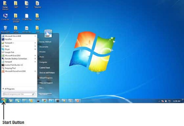
Step 2 − Click on All Programs option from the menu.

Step 3 − Search for Microsoft Office from the sub menu and click it.

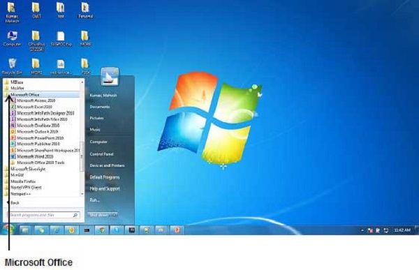
Step 4 − Search for Microsoft Excel 2010 from the submenu and click it.

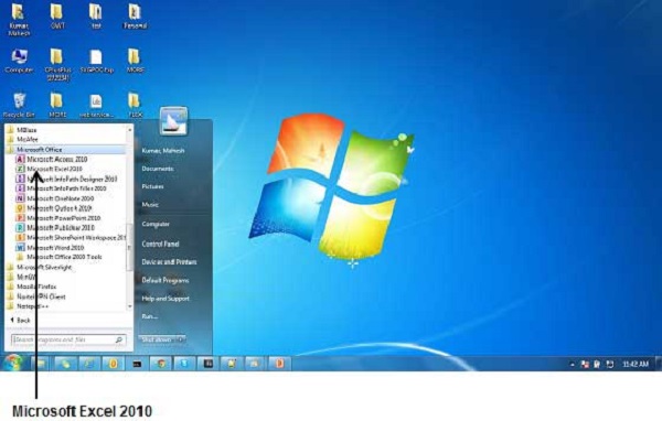
This will launch the Microsoft Excel 2010 application and you will see the following excel window.

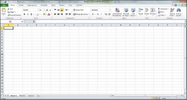
Explore Window in Excel 2010

The following basic window appears when you start the excel application. Let us now understand the various important parts of this window.

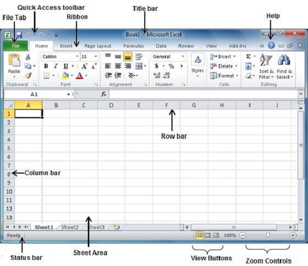
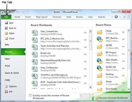
File Tab

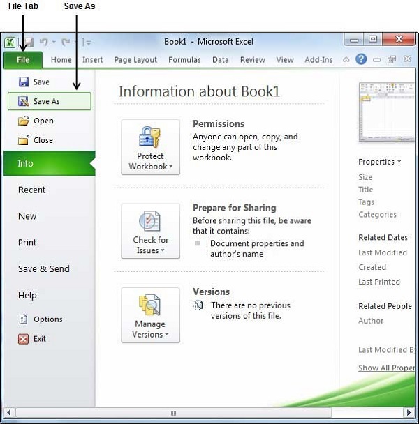
The File tab replaces the Office button from Excel 2007. You can click it to check the Backstage view, where you come when you need to open or save files, create new sheets, print a sheet, and do other file-related operations.

Quick Access Toolbar

You will find this toolbar just above the File tab and its purpose is to provide a convenient resting place for the Excel’s most frequently used commands. You can customize this toolbar based on your comfort.

Ribbon

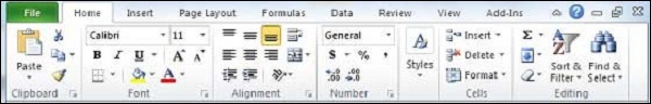
Ribbon contains commands organized in three components −

Tabs − They appear across the top of the Ribbon and contain groups of related commands. Home, Insert, Page Layout are the examples of ribbon tabs.
Groups − They organize related commands; each group name appears below the group on the Ribbon. For example, group of commands related to fonts or group of commands related to alignment etc.
Commands − Commands appear within each group as mentioned above.

Title Bar

This lies in the middle and at the top of the window. Title bar shows the program and the sheet titles.

Help

The Help Icon can be used to get excel related help anytime you like. This provides nice tutorial on various subjects related to excel.

Zoom Control

Zoom control lets you zoom in for a closer look at your text. The zoom control consists of a slider that you can slide left or right to zoom in or out. The + buttons can be clicked to increase or decrease the zoom factor.

View Buttons

The group of three buttons located to the left of the Zoom control, near the bottom of the screen, lets you switch among excel’s various sheet views.

Normal Layout view − This displays the page in normal view.
Page Layout view − This displays pages exactly as they will appear when printed. This gives a full screen look of the document.
Page Break view − This shows a preview of where pages will break when printed.

Sheet Area

The area where you enter data. The flashing vertical bar is called the insertion point and it represents the location where text will appear when you type.

Row Bar

Rows are numbered from 1 onwards and keeps on increasing as you keep entering data. Maximum limit is 1,048,576 rows.

Column Bar

Columns are numbered from A onwards and keeps on increasing as you keep entering data. After Z, it will start the series of AA, AB and so on. Maximum limit is 16,384 columns.

Status Bar

This displays the current status of the active cell in the worksheet. A cell can be in either of the fours states (a) Ready mode which indicates that the worksheet is ready to accept user inpu (b) Edit mode indicates that cell is editing mode, if it is not activated the you can activate editing mode by double-clicking on a cell (c) A cell enters into Enter mode when a user types data into a cell (d) Point mode triggers when a formula is being entered using a cell reference by mouse pointing or the arrow keys on the keyboard.

Dialog Box Launcher

This appears as a very small arrow in the lower-right corner of many groups on the Ribbon. Clicking this button opens a dialog box or task pane that provides more options about the group.

BackStage View in Excel 2010

The Backstage view has been introduced in Excel 2010 and acts as the central place for managing your sheets. The backstage view helps in creating new sheets, saving and opening sheets, printing and sharing sheets, and so on.

Getting to the Backstage View is easy. Just click the File tab located in the upper-left corner of the Excel Ribbon. If you already do not have any opened sheet then you will see a window listing down all the recently opened sheets as follows −

If you already have an opened sheet then it will display a window showing the details about the opened sheet as shown below. Backstage view shows three columns when you select most of the available options in the first column.

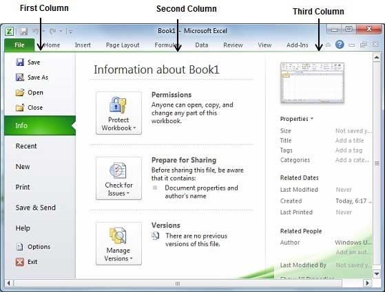
First column of the backstage view will have the following options −

S.No.	Option & Description
1	Save If an existing sheet is opened, it would be saved as is, otherwise it will display a dialogue box asking for the sheet name.
2	Save As A dialogue box will be displayed asking for sheet name and sheet type. By default, it will save in sheet 2010 format with extension .xlsx.
3	Open This option is used to open an existing excel sheet.
4	Close This option is used to close an opened sheet.
5	Info This option displays the information about the opened sheet.
6	Recent This option lists down all the recently opened sheets.
7	New This option is used to open a new sheet.
8	Print This option is used to print an opened sheet.
9	Save & Send This option saves an opened sheet and displays options to send the sheet using email etc.
10	Help You can use this option to get the required help about excel 2010.
11	Options Use this option to set various option related to excel 2010.
12	Exit Use this option to close the sheet and exit.

Sheet Information

When you click Info option available in the first column, it displays the following information in the second column of the backstage view −

Compatibility Mode − If the sheet is not a native excel 2007/2010 sheet, a Convert button appears here, enabling you to easily update its format. Otherwise, this category does not appear.
Permissions − You can use this option to protect the excel sheet. You can set a password so that nobody can open your sheet, or you can lock the sheet so that nobody can edit your sheet.
Prepare for Sharing − This section highlights important information you should know about your sheet before you send it to others, such as a record of the edits you made as you developed the sheet.
Versions − If the sheet has been saved several times, you may be able to access previous versions of it from this section.

Sheet Properties

When you click Info option available in the first column, it displays various properties in the third column of the backstage view. These properties include sheet size, title, tags, categories etc.

You can also edit various properties. Just try to click on the property value and if property is editable, then it will display a text box where you can add your text like title, tags, comments, Author.

Exit Backstage View

It is simple to exit from the Backstage View. Either click on the File tab or press the Esc button on the keyboard to go back to excel working mode.

Entering Values in Excel 2010

Entering values in excel sheet is a child’s play and this chapter shows how to enter values in an excel sheet. A new sheet is displayed by default when you open an excel sheet as shown in the below screen shot.

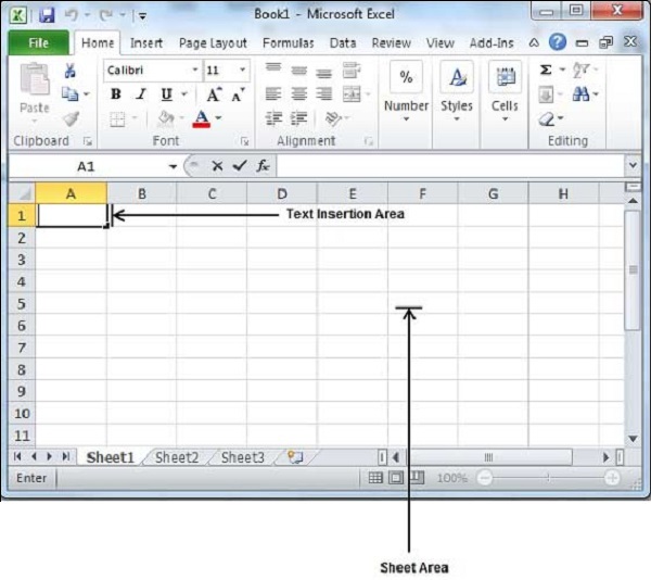
Sheet area is the place where you type your text. The flashing vertical bar is called the insertion point and it represents the location where text will appear when you type. When you click on a box then the box is highlighted. When you double click the box, the flashing vertical bar appears and you can start entering your data.

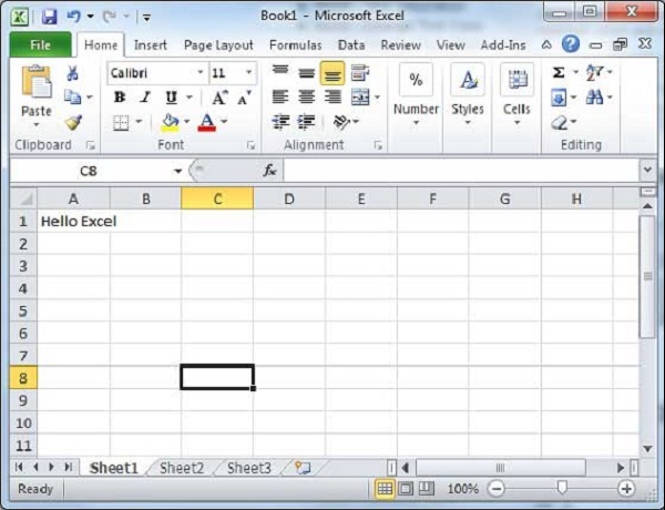
So, just keep your mouse cursor at the text insertion point and start typing whatever text you would like to type. We have typed only two words «Hello Excel» as shown below. The text appears to the left of the insertion point as you type.

There are following three important points, which would help you while typing −

Press Tab to go to next column.
Press Enter to go to next row.
Press Alt + Enter to enter a new line in the same column.

Move Around in Excel 2010

Excel provides a number of ways to move around a sheet using the mouse and the keyboard.

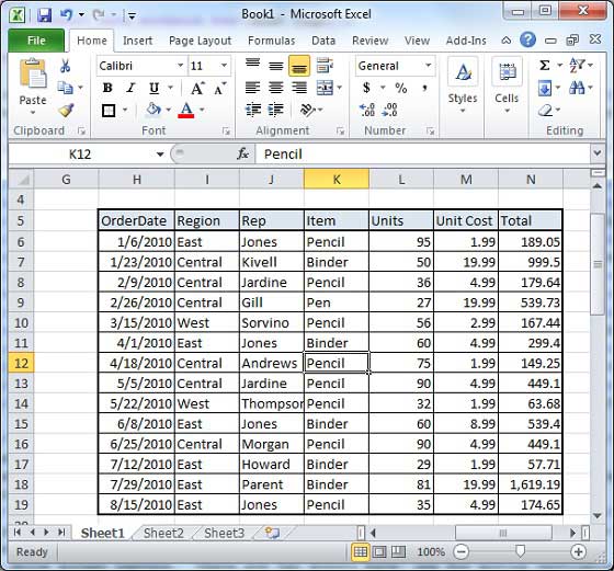
First of all, let us create some sample text before we proceed. Open a new excel sheet and type any data. We’ve shown a sample data in the screenshot.

OrderDate	Region	Rep	Item	Units	Unit Cost	Total
1/6/2010	East	Jones	Pencil	95	1.99	189.05
1/23/2010	Central	Kivell	Binder	50	19.99	999.5
2/9/2010	Central	Jardine	Pencil	36	4.99	179.64
2/26/2010	Central	Gill	Pen	27	19.99	539.73
3/15/2010	West	Sorvino	Pencil	56	2.99	167.44
4/1/2010	East	Jones	Binder	60	4.99	299.4
4/18/2010	Central	Andrews	Pencil	75	1.99	149.25
5/5/2010	Central	Jardine	Pencil	90	4.99	449.1
5/22/2010	West	Thompson	Pencil	32	1.99	63.68
6/8/2010	East	Jones	Binder	60	8.99	539.4
6/25/2010	Central	Morgan	Pencil	90	4.99	449.1
7/12/2010	East	Howard	Binder	29	1.99	57.71
7/29/2010	East	Parent	Binder	81	19.99	1,619.19
8/15/2010	East	Jones	Pencil	35	4.99	174.65

Moving with Mouse

You can easily move the insertion point by clicking in your text anywhere on the screen. Sometime if the sheet is big then you cannot see a place where you want to move. In such situations, you would have to use the scroll bars, as shown in the following screen shot −

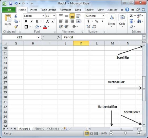
You can scroll your sheet by rolling your mouse wheel, which is equivalent to clicking the up-arrow or down-arrow buttons in the scroll bar.

Moving with Scroll Bars

As shown in the above screen capture, there are two scroll bars: one for moving vertically within the sheet, and one for moving horizontally. Using the vertical scroll bar, you may −

Move upward by one line by clicking the upward-pointing scroll arrow.
Move downward by one line by clicking the downward-pointing scroll arrow.
Move one next page, using next page button (footnote).
Move one previous page, using previous page button (footnote).
Use Browse Object button to move through the sheet, going from one chosen object to the next.

Moving with Keyboard

The following keyboard commands, used for moving around your sheet, also move the insertion point −

Keystroke	Where the Insertion Point Moves
	Forward one box
	Back one box
	Up one box
	Down one box
PageUp	To the previous screen
PageDown	To the next screen
Home	To the beginning of the current screen
End	To the end of the current screen

You can move box by box or sheet by sheet. Now click in any box containing data in the sheet. You would have to hold down the Ctrl key while pressing an arrow key, which moves the insertion point as described here −

Key Combination	Where the Insertion Point Moves
Ctrl +	To the last box containing data of the current row.
Ctrl +	To the first box containing data of the current row.
Ctrl +	To the first box containing data of the current column.
Ctrl +	To the last box containing data of the current column.
Ctrl + PageUp	To the sheet in the left of the current sheet.
Ctrl + PageDown	To the sheet in the right of the current sheet.
Ctrl + Home	To the beginning of the sheet.
Ctrl + End	To the end of the sheet.

Moving with Go To Command

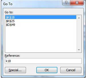
Press F5 key to use Go To command, which will display a dialogue box where you will find various options to reach to a particular box.

Normally, we use row and column number, for example K5 and finally press Go To button.

Save Workbook in Excel 2010

Saving New Sheet

Once you are done with typing in your new excel sheet, it is time to save your sheet/workbook to avoid losing work you have done on an Excel sheet. Following are the steps to save an edited excel sheet −

Step 1 − Click the File tab and select Save As option.

Step 2 − Select a folder where you would like to save the sheet, Enter file name, which you want to give to your sheet and Select a Save as type, by default it is .xlsx format.

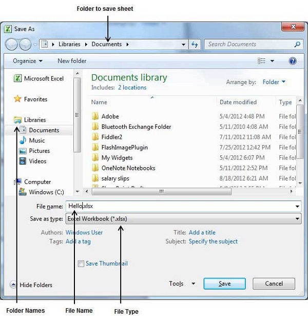
Step 3 − Finally, click on Save button and your sheet will be saved with the entered name in the selected folder.

Saving New Changes

There may be a situation when you open an existing sheet and edit it partially or completely, or even you would like to save the changes in between editing of the sheet. If you want to save this sheet with the same name, then you can use either of the following simple options −

Just press Ctrl + S keys to save the changes.
Optionally, you can click on the floppy icon available at the top left corner and just above the File tab. This option will also save the changes.
You can also use third method to save the changes, which is the Save option available just above the Save As option as shown in the above screen capture.

If your sheet is new and it was never saved so far, then with either of the three options, word would display you a dialogue box to let you select a folder, and enter sheet name as explained in case of saving new sheet.

Create Worksheet in Excel 2010

Creating New Worksheet

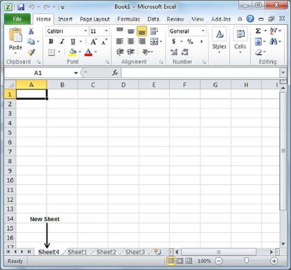
Three new blank sheets always open when you start Microsoft Excel. Below steps explain you how to create a new worksheet if you want to start another new worksheet while you are working on a worksheet, or you closed an already opened worksheet and want to start a new worksheet.

Step 1 − Right Click the Sheet Name and select Insert option.

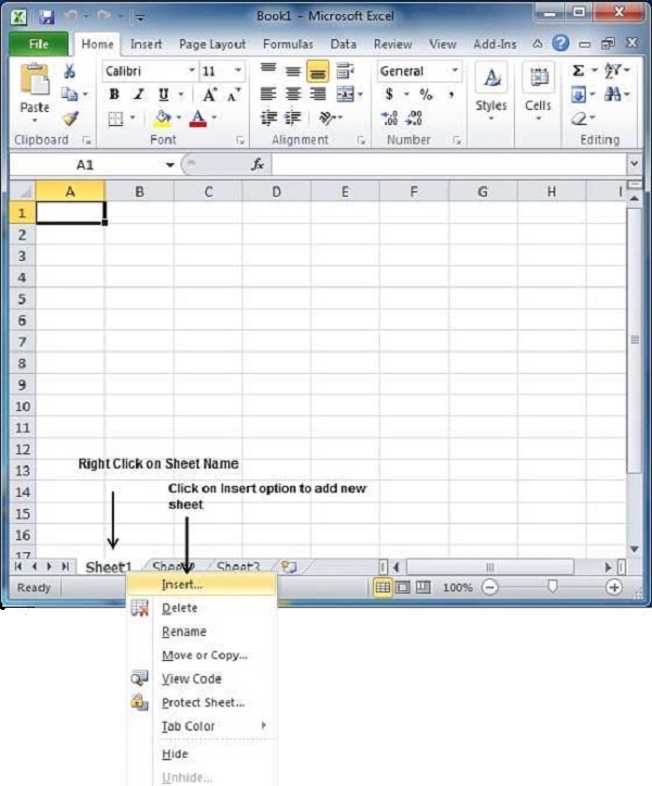
Step 2 − Now you’ll see the Insert dialog with select Worksheet option as selected from the general tab. Click the Ok button.

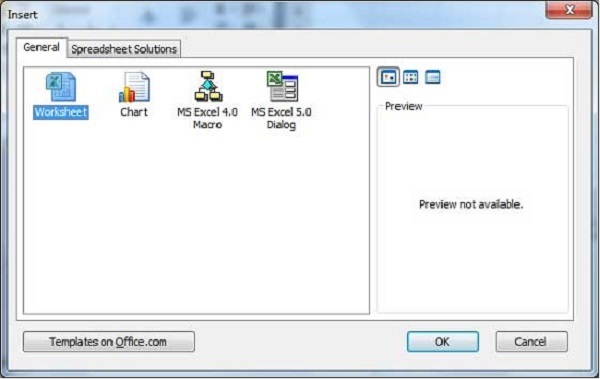
Now you should have your blank sheet as shown below ready to start typing your text.

You can use a short cut to create a blank sheet anytime. Try using the Shift+F11 keys and you will see a new blank sheet similar to the above sheet is opened.

Copy Worksheet in Excel 2010

Copy Worksheet

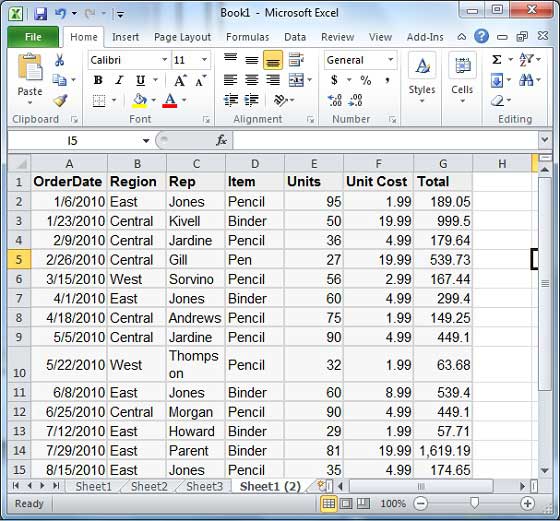
First of all, let us create some sample text before we proceed. Open a new excel sheet and type any data. We’ve shown a sample data in the screenshot.

OrderDate	Region	Rep	Item	Units	Unit Cost	Total
1/6/2010	East	Jones	Pencil	95	1.99	189.05
1/23/2010	Central	Kivell	Binder	50	19.99	999.5
2/9/2010	Central	Jardine	Pencil	36	4.99	179.64
2/26/2010	Central	Gill	Pen	27	19.99	539.73
3/15/2010	West	Sorvino	Pencil	56	2.99	167.44
4/1/2010	East	Jones	Binder	60	4.99	299.4
4/18/2010	Central	Andrews	Pencil	75	1.99	149.25
5/5/2010	Central	Jardine	Pencil	90	4.99	449.1
5/22/2010	West	Thompson	Pencil	32	1.99	63.68
6/8/2010	East	Jones	Binder	60	8.99	539.4
6/25/2010	Central	Morgan	Pencil	90	4.99	449.1
7/12/2010	East	Howard	Binder	29	1.99	57.71
7/29/2010	East	Parent	Binder	81	19.99	1,619.19
8/15/2010	East	Jones	Pencil	35	4.99	174.65

Here are the steps to copy an entire worksheet.

Step 1 − Right Click the Sheet Name and select the Move or Copy option.

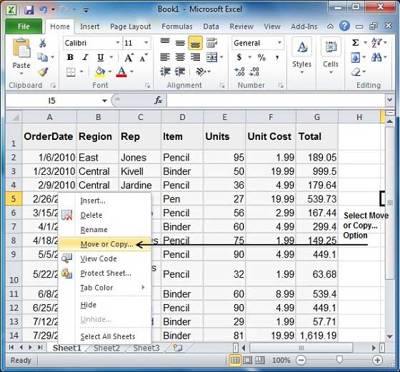
Step 2 − Now you’ll see the Move or Copy dialog with select Worksheet option as selected from the general tab. Click the Ok button.

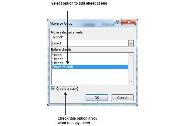
Select Create a Copy Checkbox to create a copy of the current sheet and Before sheet option as (move to end) so that new sheet gets created at the end.

Press the Ok Button.

Now you should have your copied sheet as shown below.

You can rename the sheet by double clicking on it. On double click, the sheet name becomes editable. Enter any name say Sheet5 and press Tab or Enter Key.

Hiding Worksheet in Excel 2010

Hiding Worksheet

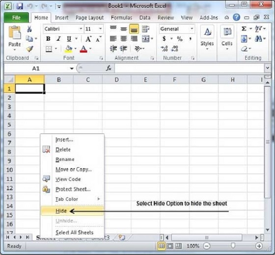
Here is the step to hide a worksheet.

Step − Right Click the Sheet Name and select the Hide option. Sheet will get hidden.

Unhiding Worksheet

Here are the steps to unhide a worksheet.

Step 1 − Right Click on any Sheet Name and select the Unhide… option.

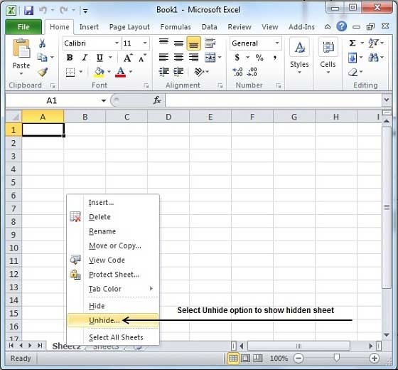
Step 2 − Select Sheet Name to unhide in Unhide dialog to unhide the sheet.

Press the Ok Button.

Now you will have your hidden sheet back.

Delete Worksheet in Excel 2010

Delete Worksheet

Here is the step to delete a worksheet.

Step − Right Click the Sheet Name and select the Delete option.

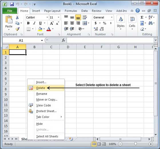
Sheet will get deleted if it is empty, otherwise you’ll see a confirmation message.

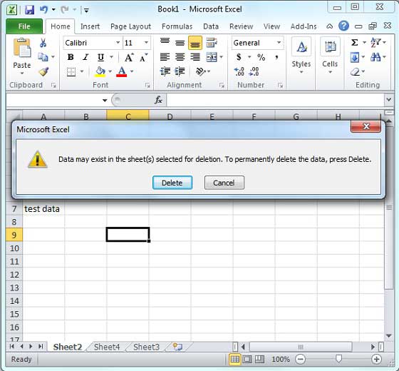
Press the Delete Button.

Now your worksheet will get deleted.

Close Workbook in Excel 2010

Close Workbook

Here are the steps to close a workbook.

Step 1 − Click the Close Button as shown below.

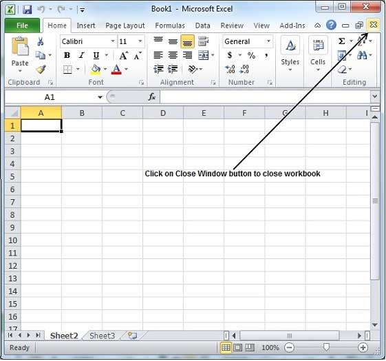
You’ll see a confirmation message to save the workbook.

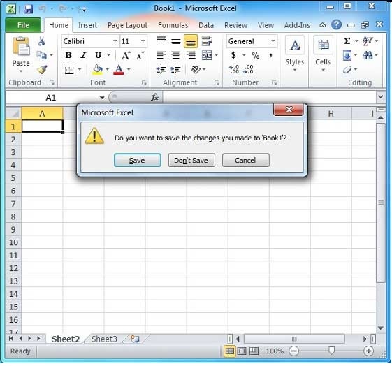
Step 2 − Press the Save Button to save the workbook as we did in MS Excel — Save Workbook chapter.

Now your worksheet will get closed.

Open Workbook in Excel 2010

Let us see how to open workbook from excel in the below mentioned steps.

Step 1 − Click the File Menu as shown below. You can see the Open option in File Menu.

There are two more columns Recent workbooks and Recent places, where you can see the recently opened workbooks and the recent places from where workbooks are opened.

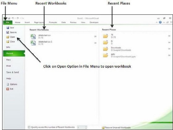
Step 2 − Clicking the Open Option will open the browse dialog as shown below. Browse the directory and find the file you need to open.

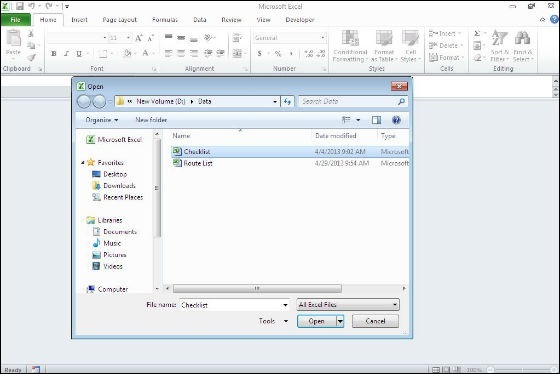
Step 3 − Once you select the workbook your workbook will be opened as below −

Context Help in Excel 2010

MS Excel provides context sensitive help on mouse over. To see context sensitive help for a particular Menu option, hover the mouse over the option for some time. Then you can see the context sensitive Help as shown below.

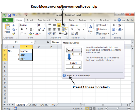
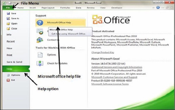
Getting More Help

For getting more help with MS Excel from Microsoft you can press F1 or by File → Help → Support → Microsoft Office Help.

Insert Data in Excel 2010

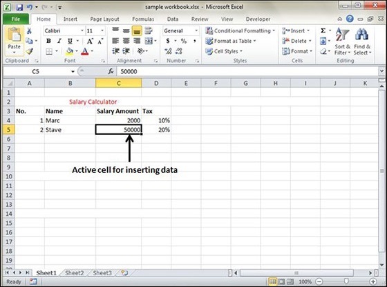
In MS Excel, there are 1048576*16384 cells. MS Excel cell can have Text, Numeric value or formulas. An MS Excel cell can have maximum of 32000 characters.

Inserting Data

For inserting data in MS Excel, just activate the cell type text or number and press enter or Navigation keys.

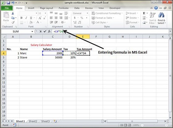
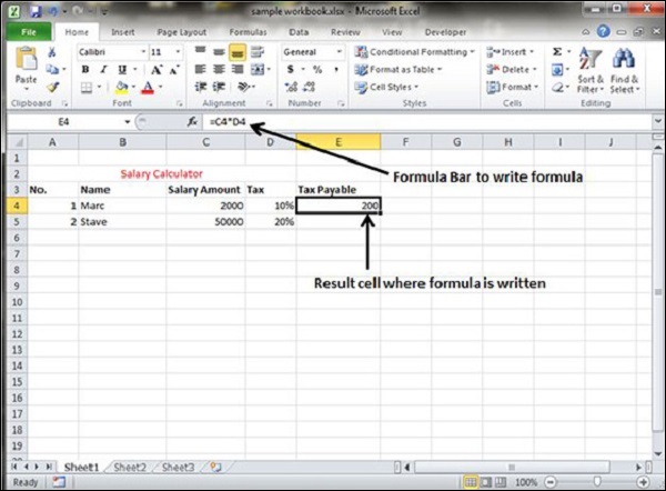
Inserting Formula

For inserting formula in MS Excel go to the formula bar, enter the formula and then press enter or navigation key. See the screen-shot below to understand it.

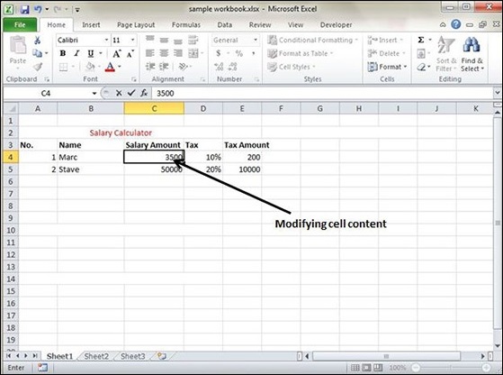
Modifying Cell Content

For modifying the cell content just activate the cell, enter a new value and then press enter or navigation key to see the changes. See the screen-shot below to understand it.

Select Data in Excel 2010

MS Excel provides various ways of selecting data in the sheet. Let us see those ways.

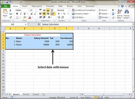
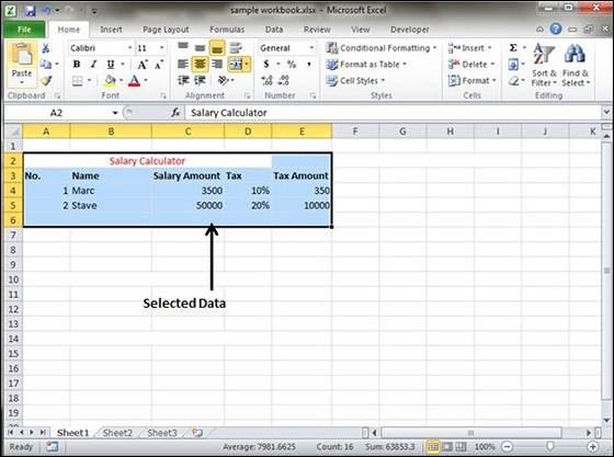
Select with Mouse

Drag the mouse over the data you want to select. It will select those cells as shown below.

Select with Special

If you want to select specific region, select any cell in that region. Pressing F5 will show the below dialogue box.

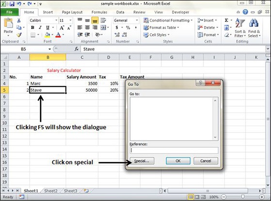
Click on Special button to see the below dialogue box. Select current region from the radio buttons. Click on ok to see the current region selected.

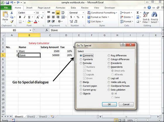
As you can see in the below screen, the data is selected for the current region.

Delete Data in Excel 2010

MS Excel provides various ways of deleting data in the sheet. Let us see those ways.

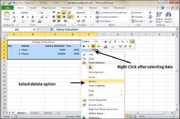
Delete with Mouse

Select the data you want to delete. Right Click on the sheet. Select the delete option, to delete the data.

Delete with Delete Key

Select the data you want to delete. Press on the Delete Button from the keyboard, it will delete the data.

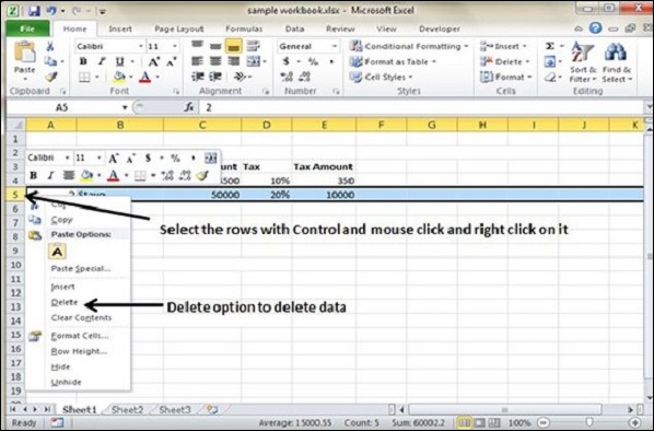
Selective Delete for Rows

Select the rows, which you want to delete with Mouse click + Control Key. Then right click to show the various options. Select the Delete option to delete the selected rows.

Move Data in Excel 2010

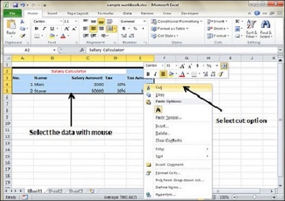
Let us see how we can Move Data with MS Excel.

Step 1 − Select the data you want to Move. Right Click and Select the cut option.

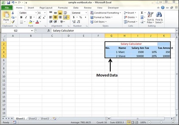
Step 2 − Select the first cell where you want to move the data. Right click on it and paste the data. You can see the data is moved now.

Rows & Columns in Excel 2010

Row and Column Basics

MS Excel is in tabular format consisting of rows and columns.

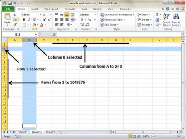
Row runs horizontally while Column runs vertically.
Each row is identified by row number, which runs vertically at the left side of the sheet.
Each column is identified by column header, which runs horizontally at the top of the sheet.

For MS Excel 2010, Row numbers ranges from 1 to 1048576; in total 1048576 rows, and Columns ranges from A to XFD; in total 16384 columns.

Navigation with Rows and Columns

Let us see how to move to the last row or the last column.

You can go to the last row by clicking Control + Down Navigation arrow.
You can go to the last column by clicking Control + Right Navigation arrow.

Cell Introduction

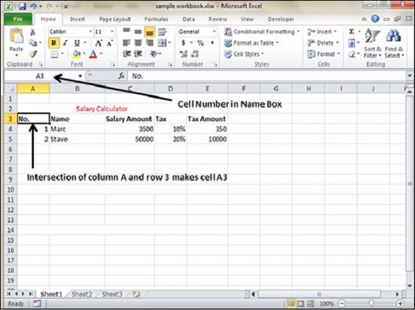
The intersection of rows and columns is called cell.

Cell is identified with Combination of column header and row number.

For example − A1, A2.

Copy & Paste in Excel 2010

MS Excel provides copy paste option in different ways. The simplest method of copy paste is as below.

Copy Paste

To copy and paste, just select the cells you want to copy. Choose copy option after right click or press Control + C.
Select the cell where you need to paste this copied content. Right click and select paste option or press Control + V.

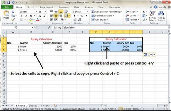
In this case, MS Excel will copy everything such as values, formulas, Formats, Comments and validation. MS Excel will overwrite the content with paste. If you want to undo this, press Control + Z from the keyboard.

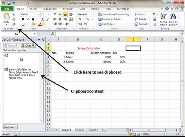
Copy Paste using Office Clipboard

When you copy data in MS Excel, it puts the copied content in Windows and Office Clipboard. You can view the clipboard content by Home → Clipboard. View the clipboard content. Select the cell where you need to paste. Click on paste, to paste the content.

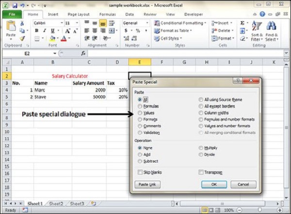
Copy Paste in Special way

You may not want to copy everything in some cases. For example, you want to copy only Values or you want to copy only the formatting of cells. Select the paste special option as shown below.

Below are the various options available in paste special.

All − Pastes the cell’s contents, formats, and data validation from the Windows Clipboard.
Formulas − Pastes formulas, but not formatting.
Values − Pastes only values not the formulas.
Formats − Pastes only the formatting of the source range.
Comments − Pastes the comments with the respective cells.
Validation − Pastes validation applied in the cells.
All using source theme − Pastes formulas, and all formatting.
All except borders − Pastes everything except borders that appear in the source range.
Column Width − Pastes formulas, and also duplicates the column width of the copied cells.
Formulas & Number Formats − Pastes formulas and number formatting only.
Values & Number Formats − Pastes the results of formulas, plus the number.
Merge Conditional Formatting − This icon is displayed only when the copied cells contain conditional formatting. When clicked, it merges the copied conditional formatting with any conditional formatting in the destination range.
Transpose − Changes the orientation of the copied range. Rows become columns, and columns become rows. Any formulas in the copied range are adjusted so that they work properly when transposed.

Find & Replace in Excel 2010

MS Excel provides Find & Replace option for finding text within the sheet.

Find and Replace Dialogue

Let us see how to access the Find & Replace Dialogue.

To access the Find & Replace, Choose Home → Find & Select → Find or press Control + F Key. See the image below.

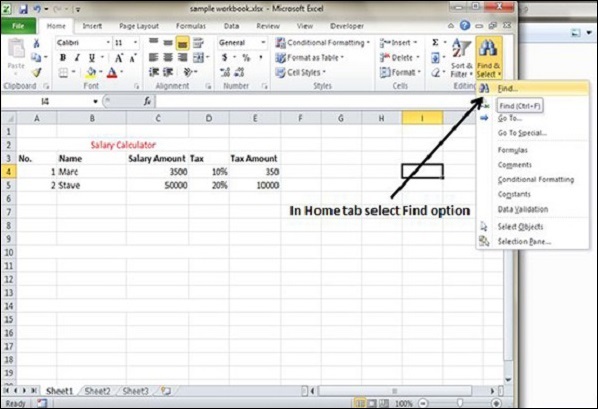
You can see the Find and Replace dialogue as below.

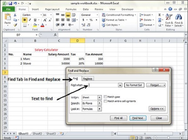
You can replace the found text with the new text in the Replace tab.

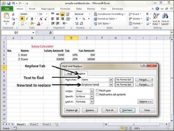
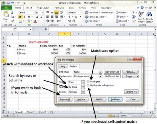
Exploring Options

Now, let us see the various options available under the Find dialogue.

Within − Specifying the search should be in Sheet or workbook.
Search By − Specifying the internal search method by rows or by columns.
Look In − If you want to find text in formula as well, then select this option.
Match Case − If you want to match the case like lower case or upper case of words, then check this option.
Match Entire Cell Content − If you want the exact match of the word with cell, then check this option.

Spell Check in Excel 2010

MS Excel provides a feature of Word Processing program called Spelling check. We can get rid of the spelling mistakes with the help of spelling check feature.

Spell Check Basis

Let us see how to access the spell check.

To access the spell checker, Choose Review ➪ Spelling or press F7.
To check the spelling in just a particular range, select the range before you activate the spell checker.
If the spell checker finds any words it does not recognize as correct, it displays the Spelling dialogue with suggested options.

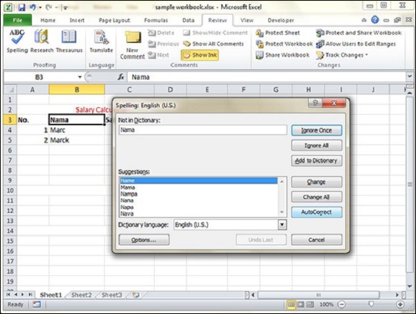
Exploring Options

Let us see the various options available in spell check dialogue.

Ignore Once − Ignores the word and continues the spell check.
Ignore All − Ignores the word and all subsequent occurrences of it.
Add to Dictionary − Adds the word to the dictionary.
Change − Changes the word to the selected word in the Suggestions list.
Change All − Changes the word to the selected word in the Suggestions list and changes all subsequent occurrences of it without asking.
AutoCorrect − Adds the misspelled word and its correct spelling (which you select from the list) to the AutoCorrect list.

Zoom In/Out in Excel 2010

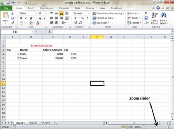
Zoom Slider

By default, everything on screen is displayed at 100% in MS Excel. You can change the zoom percentage from 10% (tiny) to 400% (huge). Zooming doesn’t change the font size, so it has no effect on the printed output.

You can view the zoom slider at the right bottom of the workbook as shown below.

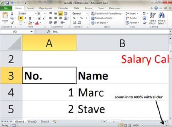
Zoom In

You can zoom in the workbook by moving the slider to the right. It will change the only view of the workbook. You can have maximum of 400% zoom in. See the below screen-shot.

Zoom In

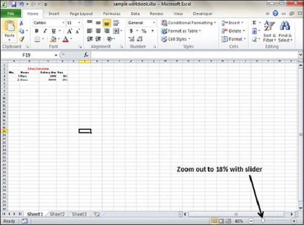
Zoom Out

You can zoom out the workbook by moving the slider to the left. It will change the only view of the workbook. You can have maximum of 10% zoom in. See the below screen-shot.

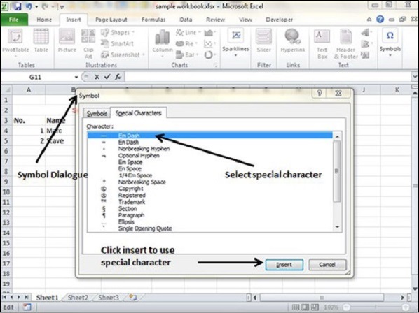
Special Symbols in Excel 2010

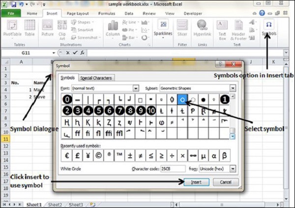
If you want to insert some symbols or special characters that are not found on the keyboard in that case you need to use the Symbols option.

Using Symbols

Go to Insert » Symbols » Symbol to view available symbols. You can see many symbols available there like Pi, alpha, beta, etc.

Select the symbol you want to add and click insert to use the symbol.

Symbols

Using Special Characters

Go to Insert » Symbols » Special Characters to view the available special characters. You can see many special characters available there like Copyright, Registered etc.

Select the special character you want to add and click insert, to use the special character.

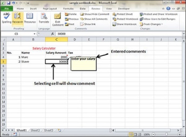
Insert Comments in Excel 2010

Adding Comment to Cell

Adding comment to cell helps in understanding the purpose of cell, what input it should have, etc. It helps in proper documentation.

To add comment to a cell, select the cell and perform any of the actions mentioned below.

Choose Review » Comments » New Comment.
Right-click the cell and choose Insert Comment from available options.
Press Shift+F2.

Initially, a comment consists of Computer’s user name. You have to modify it with text for the cell comment.

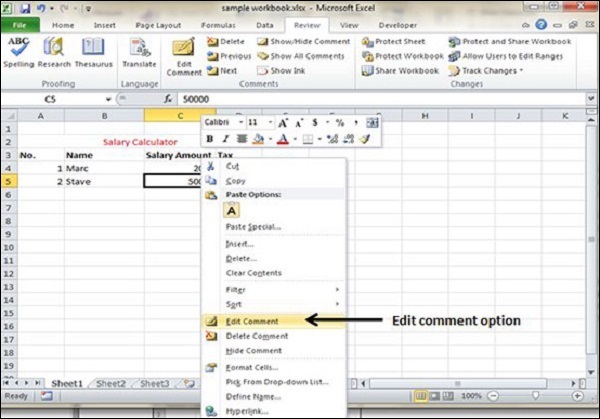
Modifying Comment

You can modify the comment you have entered before as mentioned below.

Select the cell on which the comment appears.
Right-click the cell and choose the Edit Comment from the available options.
Modify the comment.

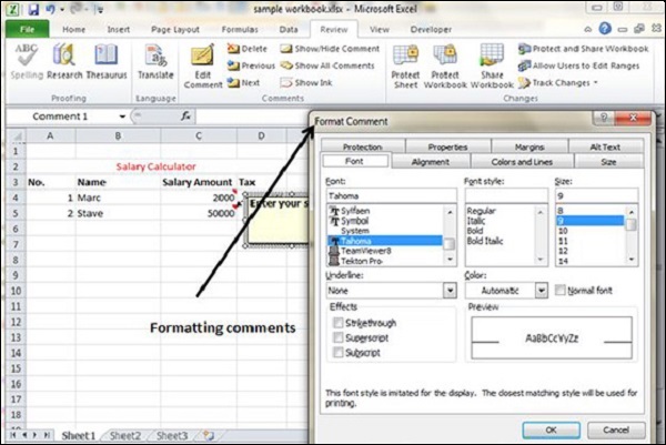
Formatting Comment

Various formatting options are available for comments. For formatting a comment, Right click on cell » Edit comment » Select comment » Right click on it » Format comment. With formatting of comment you can change the color, font, size, etc of the comment.

Add Text Box in Excel 2010

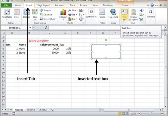
Text Boxes

Text boxes are special graphic objects that combine the text with a rectangular graphic object. Text boxes and cell comments are similar in displaying the text in rectangular box. But text boxes are always visible, while cell comments become visible after selecting the cell.

Adding Text Boxes

To add a text box, perform the below actions.

Choose Insert » Text Box » choose text box or draw it.

Initially, the comment consists of Computer’s user name. You have to modify it with text for the cell comment.

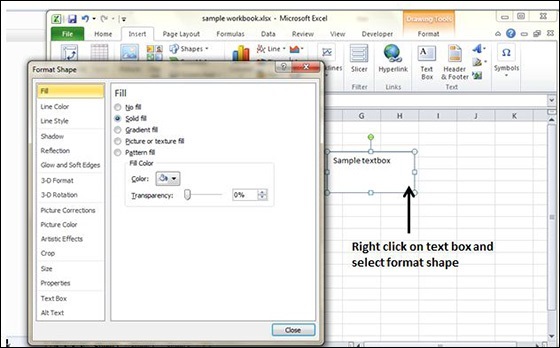
Formatting Text Box

After you have added the text box, you can format it by changing the font, font size, font style, and alignment, etc. Let us see some of the important options of formatting a text box.

Fill − Specifies the filling of text box like No fill, solid fill. Also specifying the transparency of text box fill.
Line Colour − Specifies the line colour and transparency of the line.
Line Style − Specifies the line style and width.
Size − Specifies the size of the text box.
Properties − Specifies some properties of the text box.
Text Box − Specifies text box layout, Auto-fit option and internal margins.

Undo Changes in Excel 2010

Undo Changes

You can reverse almost every action in Excel by using the Undo command. We can undo changes in following two ways.

From the Quick access tool-bar » Click Undo.
Press Control + Z.

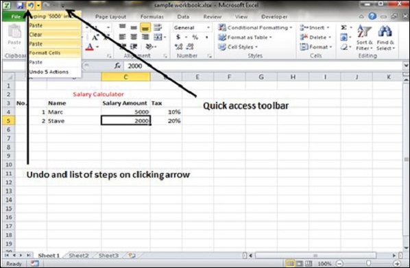
You can reverse the effects of the past 100 actions that you performed by executing Undo more than once. If you click the arrow on the right side of the Undo button, you see a list of the actions that you can reverse. Click an item in that list to undo that action and all the subsequent actions you performed.

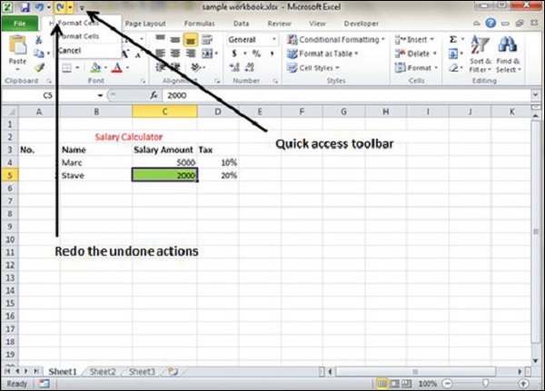
Redo Changes

You can again reverse back the action done with undo in Excel by using the Redo command. We can redo changes in following two ways.

From the Quick access tool-bar » Click Redo.
Press Control + Y.

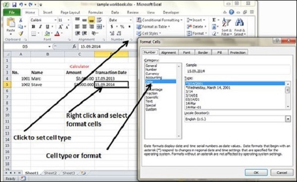
Setting Cell Type in Excel 2010

Formatting Cell

MS Excel Cell can hold different types of data like Numbers, Currency, Dates, etc. You can set the cell type in various ways as shown below −

Right Click on the cell » Format cells » Number.
Click on the Ribbon from the ribbon.

Various Cell Formats

Below are the various cell formats.

General − This is the default cell format of Cell.
Number − This displays cell as number with separator.
Currency − This displays cell as currency i.e. with currency sign.
Accounting − Similar to Currency, used for accounting purpose.
Date − Various date formats are available under this like 17-09-2013, 17^th-Sep-2013, etc.
Time − Various Time formats are available under this, like 1.30PM, 13.30, etc.
Percentage − This displays cell as percentage with decimal places like 50.00%.
Fraction − This displays cell as fraction like 1/4, 1/2 etc.
Scientific − This displays cell as exponential like 5.6E+01.
Text − This displays cell as normal text.
Special − Special formats of cell like Zip code, Phone Number.
Custom − You can use custom format by using this.

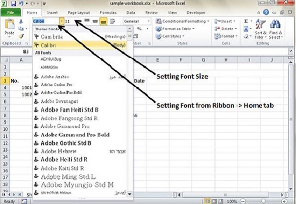
Setting Fonts in Excel 2010

You can assign any of the fonts that is installed for your printer to cells in a worksheet.

Setting Font from Home

You can set the font of the selected text from Home » Font group » select the font.

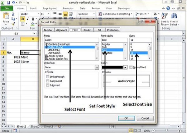
Setting Font From Format Cell Dialogue

Right click on cell » Format cells » Font Tab
Press Control + 1 or Shift + Control + F

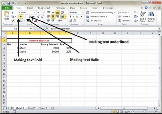
Text Decoration in Excel 2010

You can change the text decoration of the cell to change its look and feel.

Text Decoration

Various options are available in Home tab of the ribbon as mentioned below.

Bold − It makes the text in bold by choosing Home » Font Group » Click B or Press Control + B.
Italic − It makes the text italic by choosing Home » Font Group » Click I or Press Control + I.
Underline − It makes the text to be underlined by choosing Home » Font Group » Click U or Press Control + U.
Double Underline − It makes the text highlighted as double underlined by choose Home » Font Group » Click arrow near U » Select Double Underline.

More Text Decoration Options

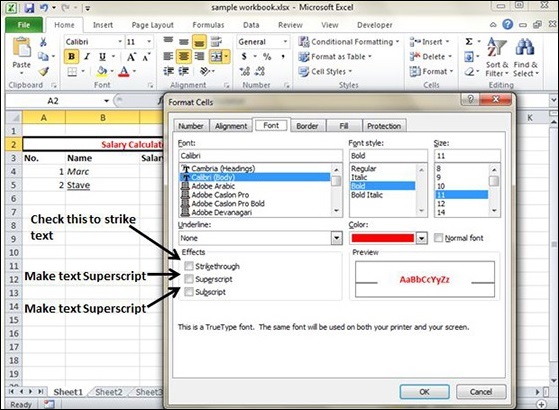
There are more options available for text decoration in Formatting cells » Font Tab »Effects cells as mentioned below.

Strike-through − It strikes the text in the center vertically.
Super Script − It makes the content to appear as a super script.
Sub Script − It makes content to appear as a sub script.

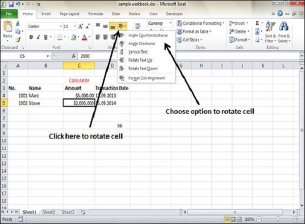
Rotate Cells in Excel 2010

You can rotate the cell by any degree to change the orientation of the cell.

Rotating Cell from Home Tab

Click on the orientation in the Home tab. Choose options available like Angle CounterClockwise, Angle Clockwise, etc.

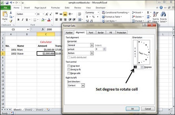
Rotating Cell from Formatting Cell

Right Click on the cell. Choose Format cells » Alignment » Set the degree for rotation.

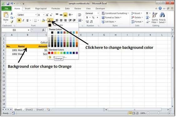
Setting Colors in Excel 2010

You can change the background color of the cell or text color.

Changing Background Color

By default the background color of the cell is white in MS Excel. You can change it as per your need from Home tab » Font group » Background color.

Changing Foreground Color

By default, the foreground or text color is black in MS Excel. You can change it as per your need from Home tab » Font group » Foreground color.

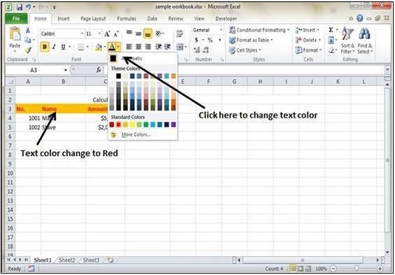
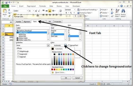
Also you can change the foreground color by selecting the cell Right click » Format cells » Font Tab » Color.

Text Alignments in Excel 2010

If you don’t like the default alignment of the cell, you can make changes in the alignment of the cell. Below are the various ways of doing it.

Change Alignment from Home Tab

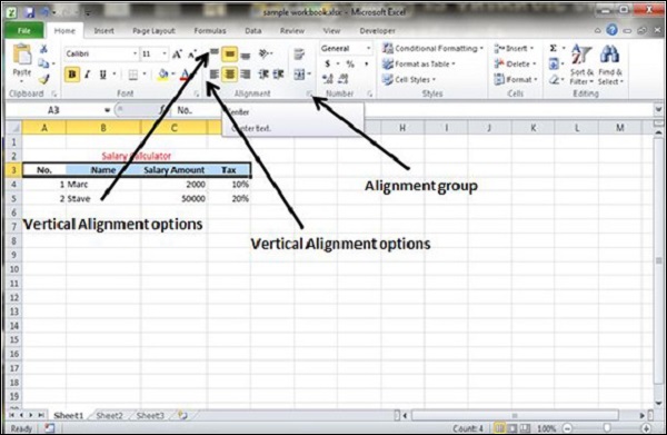
You can change the Horizontal and vertical alignment of the cell. By default, Excel aligns numbers to the right and text to the left. Click on the available option in the Alignment group in Home tab to change alignment.

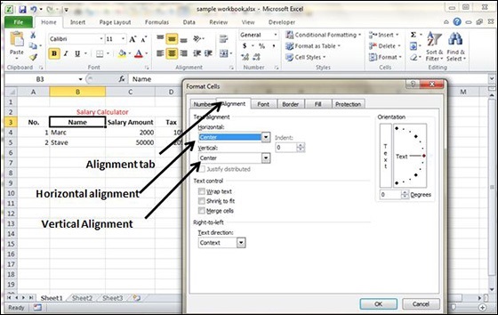
Change Alignment from Format Cells

Right click on the cell and choose format cell. In format cells dialogue, choose Alignment Tab. Select the available options from the Vertical alignment and Horizontal alignment options.

Exploring Alignment Options

1. Horizontal Alignment − You can set horizontal alignment to Left, Centre, Right, etc.

Left − Aligns the cell contents to the left side of the cell.
Center − Centers the cell contents in the cell.
Right − Aligns the cell contents to the right side of the cell.
Fill − Repeats the contents of the cell until the cell’s width is filled.
Justify − Justifies the text to the left and right of the cell. This option is applicable only if the cell is formatted as wrapped text and uses more than one line.

2. Vertical Alignment − You can set Vertical alignment to top, Middle, bottom, etc.

Top Aligns the cell contents to the top of the cell.
Center Centers the cell contents vertically in the cell.
Bottom Aligns the cell contents to the bottom of the cell.
Justify Justifies the text vertically in the cell; this option is applicable only if the cell is formatted as wrapped text and uses more than one line.

Merge & Wrap in Excel 2010

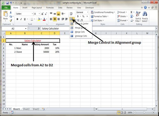
Merge Cells

MS Excel enables you to merge two or more cells. When you merge cells, you don’t combine the contents of the cells. Rather, you combine a group of cells into a single cell that occupies the same space.

You can merge cells by various ways as mentioned below.

Choose Merge & Center control on the Ribbon, which is simpler. To merge cells, select the cells that you want to merge and then click the Merge & Center button.

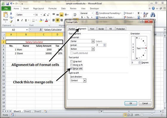
Choose Alignment tab of the Format Cells dialogue box to merge the cells.

Additional Options

The Home » Alignment group » Merge & Center control contains a drop-down list with these additional options −

Merge Across − When a multi-row range is selected, this command creates multiple merged cells — one for each row.
Merge Cells − Merges the selected cells without applying the Center attribute.
Unmerge Cells − Unmerges the selected cells.

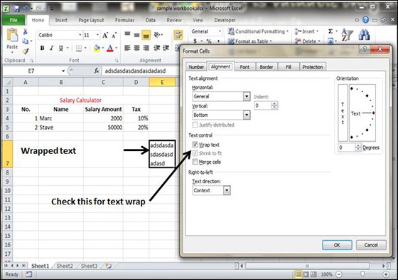
Wrap Text and Shrink to Fit

If the text is too wide to fit the column width but don’t want that text to spill over into adjacent cells, you can use either the Wrap Text option or the Shrink to Fit option to accommodate that text.

Borders and Shades in Excel 2010

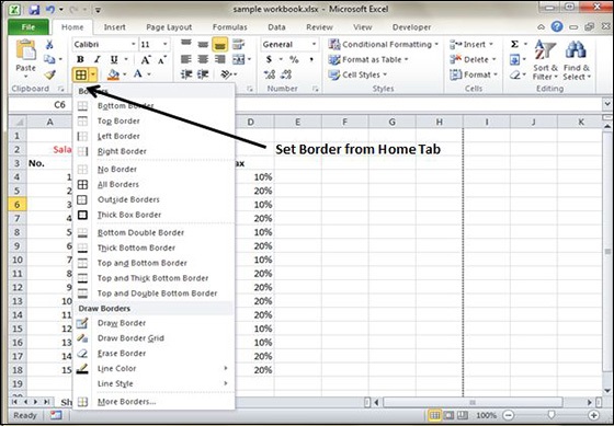
Apply Borders

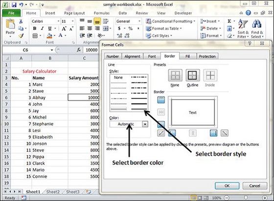
MS Excel enables you to apply borders to the cells. For applying border, select the range of cells Right Click » Format cells » Border Tab » Select the Border Style.

Then you can apply border by Home Tab » Font group »Apply Borders.

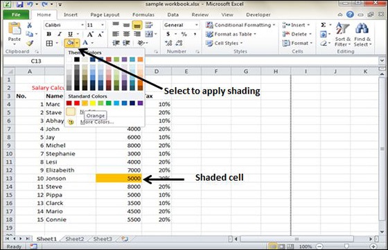
Apply Shading

You can add shading to the cell from the Home tab » Font Group » Select the Color.

Apply Formatting in Excel 2010

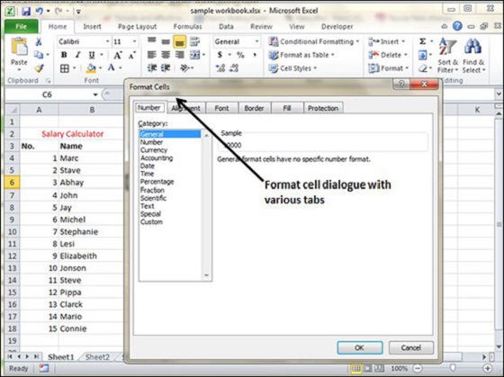
Formatting Cells

In MS Excel, you can apply formatting to the cell or range of cells by Right Click » Format cells » Select the tab. Various tabs are available as shown below

Alternative to Placing Background

Number − You can set the Format of the cell depending on the cell content. Find tutorial on this at MS Excel — Setting Cell Type.
Alignment − You can set the alignment of text on this tab. Find tutorial on this at MS Excel — Text Alignments.
Font − You can set the Font of text on this tab.Find tutorial on this at MS Excel — Setting Fonts.
Border − You can set border of cell with this tab.Find tutorial on this at MS Excel — Borders and Shades.
Fill − You can set fill of cell with this tab. Find tutorial on this at MS Excel — Borders and Shades.
Protection − You can set cell protection option with this tab.

Sheet Options in Excel 2010

Sheet Options

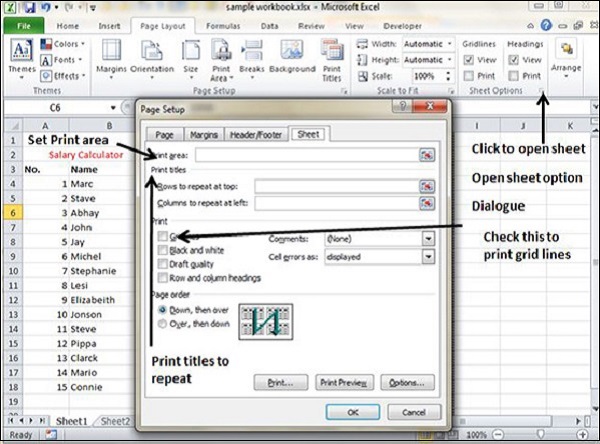
MS Excel provides various sheet options for printing purpose like generally cell gridlines aren’t printed. If you want your printout to include the gridlines, Choose Page Layout » Sheet Options group » Gridlines » Check Print.

Options in Sheet Options Dialogue

Print Area − You can set the print area with this option.
Print Titles − You can set titles to appear at the top for rows and at the left for columns.
Print −
- Gridlines − Gridlines to appear while printing worksheet.
- Black & White − Select this check box to have your color printer print the chart in black and white.
- Draft quality − Select this check box to print the chart using your printer’s draft-quality setting.
- Rows & Column Heading − Select this check box to have rows and column heading to print.
Page Order −
- Down, then Over − It prints the down pages first and then the right pages.
- Over, then Down − It prints right pages first and then comes to print the down pages.

Adjust Margins in Excel 2010

Margins

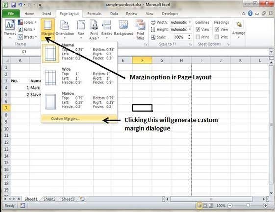
Margins are the unprinted areas along the sides, top, and bottom of a printed page. All printed pages in MS Excel have the same margins. You can’t specify different margins for different pages.

You can set margins by various ways as explained below.

Choose Page Layout » Page Setup » Margins drop-down list, you can select Normal, Wide, Narrow, or the custom Setting.

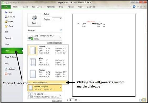
These options are also available when you choose File » Print.

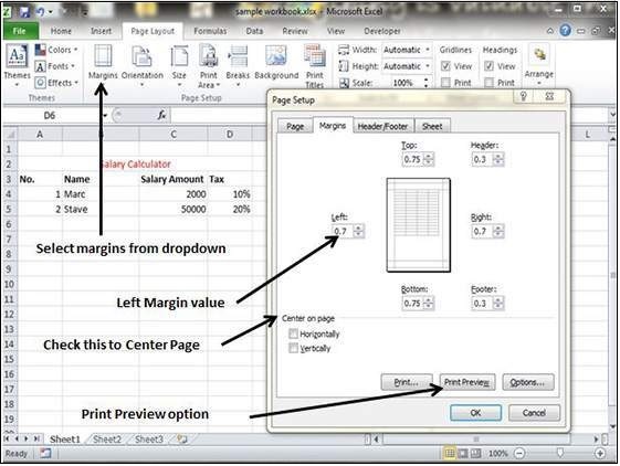
If none of these settings does the job, choose Custom Margins to display the Margins tab of the Page Setup dialog box, as shown below.

Center on Page

By default, Excel aligns the printed page at the top and left margins. If you want the output to be centered vertically or horizontally, select the appropriate check box in the Center on Page section of the Margins tab as shown in the above screenshot.

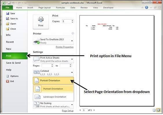
Page Orientation in Excel 2010

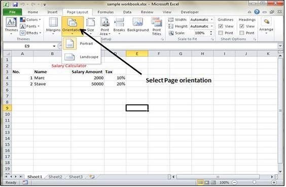
Page Orientation

Page orientation refers to how output is printed on the page. If you change the orientation, the onscreen page breaks adjust automatically to accommodate the new paper orientation.

Types of Page Orientation

Portrait − Portrait to print tall pages (the default).
Landscape − Landscape to print wide pages. Landscape orientation is useful when you have a wide range that doesn’t fit on a vertically oriented page.

Changing Page Orientation

Choose Page Layout » Page Setup » Orientation » Portrait or Landscape.

Choose File » Print.

Header and Footer in Excel 2010

Header and Footer

A header is the information that appears at the top of each printed page and a footer is the information that appears at the bottom of each printed page. By default, new workbooks do not have headers or footers.

Adding Header and Footer

Choose Page Setup dialog box » Header or Footer tab.

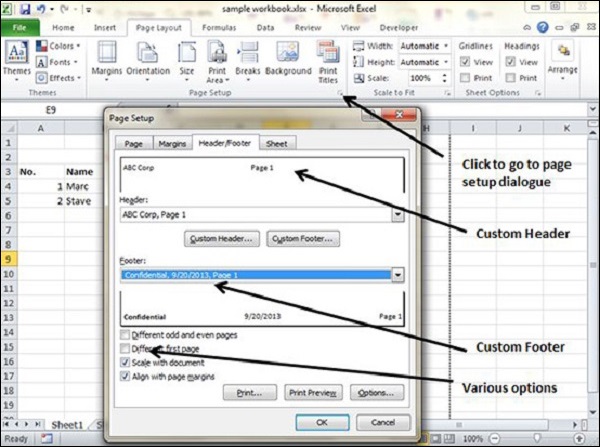
You can choose the predefined header and footer or create your custom ones.

&[Page] − Displays the page number.
&[Pages] − Displays the total number of pages to be printed.
&[Date] − Displays the current date.
&[Time] − Displays the current time.
&[Path]&[File] − Displays the workbook’s complete path and filename.
&[File] − Displays the workbook name.
&[Tab] − Displays the sheet’s name.

Other Header and Footer Options

When a header or footer is selected in Page Layout view, the Header & Footer » Design » Options group contains controls that let you specify other options −

Different First Page − Check this to specify a different header or footer for the first printed page.
Different Odd & Even Pages − Check this to specify a different header or footer for odd and even pages.
Scale with Document − If checked, the font size in the header and footer will be sized. Accordingly if the document is scaled when printed. This option is enabled, by default.
Align with Page Margins − If checked, the left header and footer will be aligned with the left margin, and the right header and footer will be aligned with the right margin. This option is enabled, by default.

Insert Page Break in Excel 2010

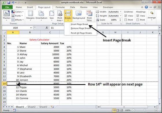
Page Breaks

If you don’t want a row to print on a page by itself or you don’t want a table header row to be the last line on a page. MS Excel gives you precise control over page breaks.

MS Excel handles page breaks automatically, but sometimes you may want to force a page break either a vertical or a horizontal one. so that the report prints the way you want.

For example, if your worksheet consists of several distinct sections, you may want to print each section on a separate sheet of paper.

Inserting Page Breaks

Insert Horizontal Page Break − For example, if you want row 14 to be the first row of a new page, select cell A14. Then choose Page Layout » Page Setup Group » Breaks» Insert Page Break.

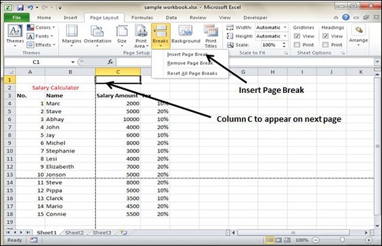
Insert vertical Page break − In this case, make sure to place the pointer in row 1. Choose Page Layout » Page Setup » Breaks » Insert Page Break to create the page break.

Removing Page Breaks

Remove a page break you’ve added − Move the cell pointer to the first row beneath the manual page break and then choose Page Layout » Page Setup » Breaks » Remove Page Break.
Remove all manual page breaks − Choose Page Layout » Page Setup » Breaks » Reset All Page Breaks.

Set Background in Excel 2010

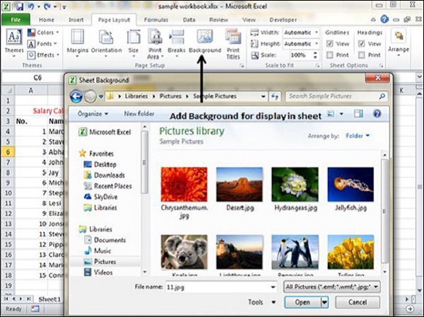
Background Image

Unfortunately, you cannot have a background image on your printouts. You may have noticed the Page Layout » Page Setup » Background command. This button displays a dialogue box that lets you select an image to display as a background. Placing this control among the other print-related commands is very misleading. Background images placed on a worksheet are never printed.

Alternative to Placing Background

You can insert a Shape, WordArt, or a picture on your worksheet and then adjust its transparency. Then copy the image to all printed pages.
You can insert an object in a page header or footer.

Freeze Panes in Excel 2010

Freezing Panes

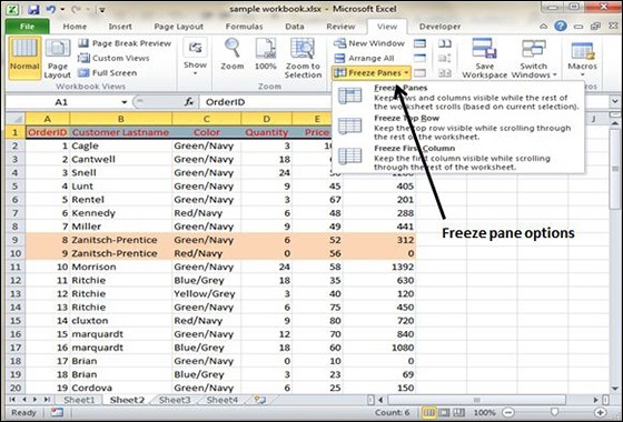
If you set up a worksheet with row or column headings, these headings will not be visible when you scroll down or to the right. MS Excel provides a handy solution to this problem with freezing panes. Freezing panes keeps the headings visible while you’re scrolling through the worksheet.

Using Freeze Panes

Follow the steps mentioned below to freeze panes.

Select the First row or First Column or the row Below, which you want to freeze, or Column right to area, which you want to freeze.
Choose View Tab » Freeze Panes.
Select the suitable option −
- Freeze Panes − To freeze area of cells.
- Freeze Top Row − To freeze first row of worksheet.
- Freeze First Column − To freeze first Column of worksheet.

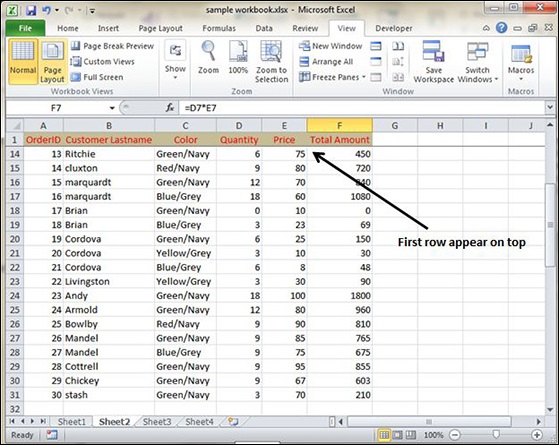
If you have selected Freeze top row you can see the first row appears at the top, after scrolling also. See the below screen-shot.

Unfreeze Panes

To unfreeze Panes, choose View Tab » Unfreeze Panes.

Conditional Format in Excel 2010

Conditional Formatting

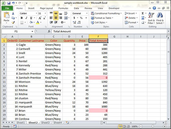
MS Excel 2010 Conditional Formatting feature enables you to format a range of values so that the values outside certain limits, are automatically formatted.

Choose Home Tab » Style group » Conditional Formatting dropdown.

Various Conditional Formatting Options

Highlight Cells Rules − It opens a continuation menu with various options for defining the formatting rules that highlight the cells in the cell selection that contain certain values, text, or dates, or that have values greater or less than a particular value, or that fall within a certain ranges of values.

Suppose you want to find cell with Amount 0 and Mark them as red.Choose Range of cell » Home Tab » Conditional Formatting DropDown » Highlight Cell Rules » Equal To.

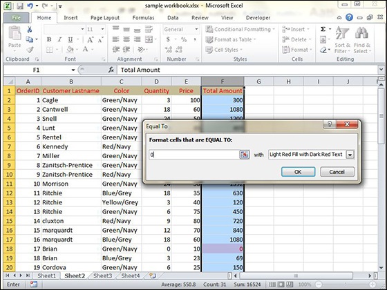
After Clicking ok, the cells with value zero are marked as red.

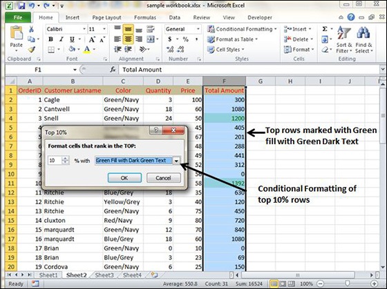
Top/Bottom Rules − It opens a continuation menu with various options for defining the formatting rules that highlight the top and bottom values, percentages, and above and below average values in the cell selection.

Suppose you want to highlight the top 10% rows you can do this with these Top/Bottom rules.

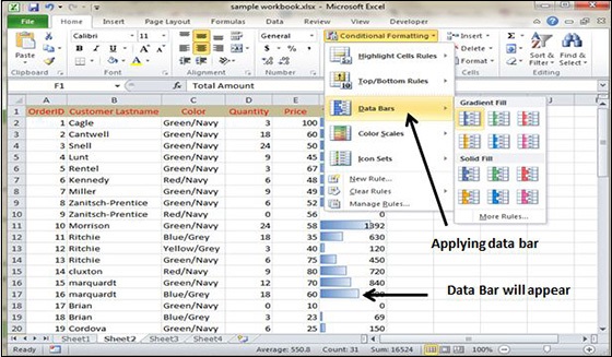
Data Bars − It opens a palette with different color data bars that you can apply to the cell selection to indicate their values relative to each other by clicking the data bar thumbnail.

With this conditional Formatting data Bars will appear in each cell.

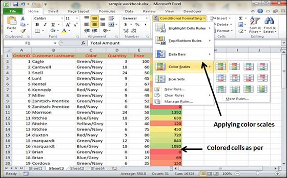
Color Scales − It opens a palette with different three- and two-colored scales that you can apply to the cell selection to indicate their values relative to each other by clicking the color scale thumbnail.

See the below screenshot with Color Scales, conditional formatting applied.

Icon Sets − It opens a palette with different sets of icons that you can apply to the cell selection to indicate their values relative to each other by clicking the icon set.

See the below screenshot with Icon Sets conditional formatting applied.

New Rule − It opens the New Formatting Rule dialog box, where you define a custom conditional formatting rule to apply to the cell selection.
Clear Rules − It opens a continuation menu, where you can remove the conditional formatting rules for the cell selection by clicking the Selected Cells option, for the entire worksheet by clicking the Entire Sheet option, or for just the current data table by clicking the This Table option.
Manage Rules − It opens the Conditional Formatting Rules Manager dialog box, where you edit and delete particular rules as well as adjust their rule precedence by moving them up or down in the Rules list box.

Creating Formulas in Excel 2010

Formulas in MS Excel

Formulas are the Bread and butter of worksheet. Without formula, worksheet will be just simple tabular representation of data. A formula consists of special code, which is entered into a cell. It performs some calculations and returns a result, which is displayed in the cell.

Formulas use a variety of operators and worksheet functions to work with values and text. The values and text used in formulas can be located in other cells, which makes changing data easy and gives worksheets their dynamic nature. For example, you can quickly change the data in a worksheet and formulas works.

Elements of Formulas

A formula can consist of any of these elements −

Mathematical operators, such as +(for addition) and *(for multiplication)

Example −
- =A1+A2 Adds the values in cells A1 and A2.
Values or text

Example −
- =200*0.5 Multiplies 200 times 0.15. This formula uses only values, and it always returns the same result as 100.
Cell references (including named cells and ranges)

Example −
- =A1=C12 Compares cell A1 with cell C12. If the cells are identical, the formula returns TRUE; otherwise, it returns FALSE.
Worksheet functions (such as SUMor AVERAGE)

Example −
- =SUM(A1:A12) Adds the values in the range A1:A12.

Creating Formula

For creating a formula you need to type in the Formula Bar. Formula begins with ‘=’ sign. When building formulas manually, you can either type in the cell addresses or you can point to them in the worksheet. Using the Pointing method to supply the cell addresses for formulas is often easier and more powerful method of formula building. When you are using built-in functions, you click the cell or drag through the cell range that you want to use when defining the function’s arguments in the Function Arguments dialog box. See the below screen shot.

As soon as you complete a formula entry, Excel calculates the result, which is then displayed inside the cell within the worksheet (the contents of the formula, however, continue to be visible on the Formula bar anytime the cell is active). If you make an error in the formula that prevents Excel from being able to calculate the formula at all, Excel displays an Alert dialog box suggesting how to fix the problem.

Copying Formulas in Excel 2010

Copying Formulas in MS Excel

Copying formulas is one of the most common tasks that you do in a typical spreadsheet that relies primarily on formulas. When a formula uses cell references rather than constant values, Excel makes the task of copying an original formula to every place that requires a similar formula.

Relative Cell Addresses

MS Excel does it automatically adjusting the cell references in the original formula to suit the position of the copies that you make. It does this through a system known as relative cell addresses, where by the column references in the cell address in the formula change to suit their new column position and the row references change to suit their new row position.

Let us see this with the help of example. Suppose we want the sum of all the rows at last, then we will write a formula for first column i.e. B. We want sum of the rows from 3 to 8 in the 9^th row.

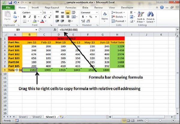
After writing formula in the 9^th row, we can drag it to remaining columns and the formula gets copied. After dragging we can see the formula in the remaining columns as below.

column C : =SUM(C3:C8)
column D : =SUM(D3:D8)
column E : =SUM(E3:E8)
column F : =SUM(F3:F8)
column G : =SUM(G3:G8)

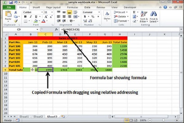
Formula Reference in Excel 2010

Cell References in Formulas

Most formulas you create include references to cells or ranges. These references enable your formulas to work dynamically with the data contained in those cells or ranges. For example, if your formula refers to cell C2 and you change the value contained in C2, the formula result reflects new value automatically. If you didn’t use references in your formulas, you would need to edit the formulas themselves in order to change the values used in the formulas.

When you use a cell (or range) reference in a formula, you can use three types of references − relative, absolute, and mixed references.

Relative Cell References

The row and column references can change when you copy the formula to another cell because the references are actually offsets from the current row and column. By default, Excel creates relative cell references in formulas.

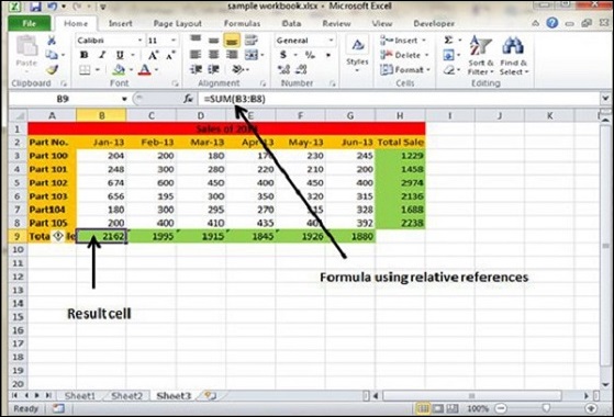
Absolute Cell References

The row and column references do not change when you copy the formula because the reference is to an actual cell address. An absolute reference uses two dollar signs in its address: one for the column letter and one for the row number (for example, $A$5).

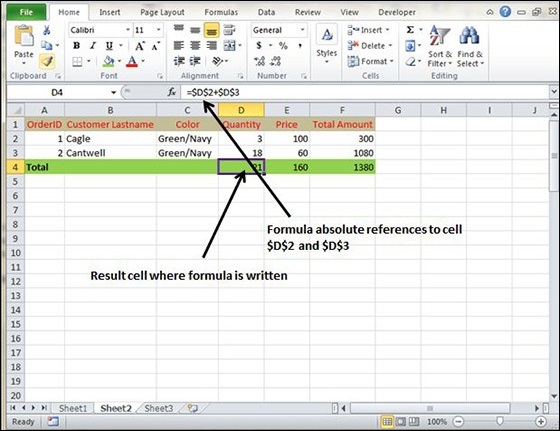
Mixed Cell References

Both the row or column reference is relative and the other is absolute. Only one of the address parts is absolute (for example, $A5 or A$5).

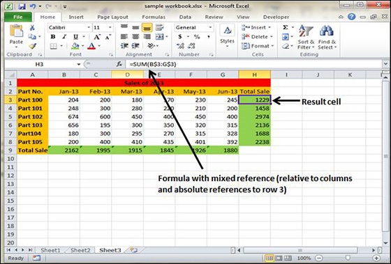
Using Functions in Excel 2010

Functions in Formula

Many formulas you create use available worksheet functions. These functions enable you to greatly enhance the power of your formulas and perform calculations that are difficult if you use only the operators. For example, you can use the LOG or SIN function to calculate the Logarithm or Sin ratio. You can’t do this complicated calculation by using the mathematical operators alone.

Using Functions

When you type = sign and then type any alphabet you will see the searched functions as below.

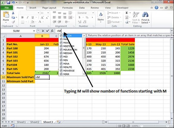
Suppose you need to determine the largest value in a range. A formula can’t tell you the answer without using a function. We will use formula that uses the MAX function to return the largest value in the range B3:B8 as =MAX(A1:D100).

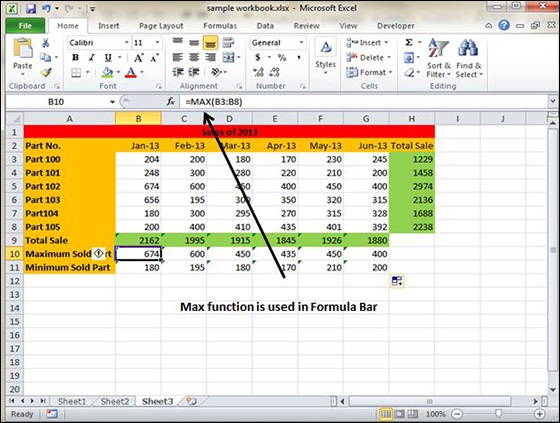
Another example of functions. Suppose you want to find if the cell of month is greater than 1900 then we can give Bonus to Sales representative. The we can achieve it with writing formula with IF functions as =IF(B9>1900,»Yes»,»No»)

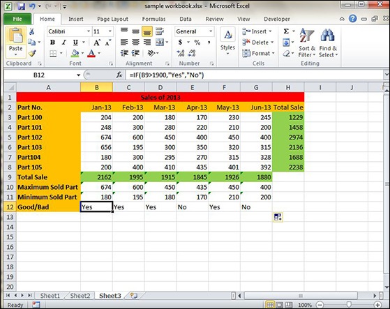
Function Arguments

In the above examples, you may have noticed that all the functions used parentheses. The information inside the parentheses is the list of arguments.

Functions vary in how they use arguments. Depending on what it has to do, a function may use.

No arguments − Examples − Now(), Date(), etc.
One argument − UPPER(), LOWER(), etc.
A fixed number of arguments − IF(), MAX(), MIN(), AVERGAGE(), etc.
Infinite number of arguments
Optional arguments

Built-in Functions in Excel 2010

Built In Functions

MS Excel has many built in functions, which we can use in our formula. To see all the functions by category, choose Formulas Tab » Insert Function. Then Insert function Dialog appears from which we can choose the function.

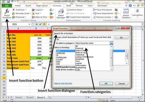
Functions by Categories

Let us see some of the built in functions in MS Excel.

Text Functions
- LOWER − Converts all characters in a supplied text string to lower case
- UPPER − Converts all characters in a supplied text string to upper case
- TRIM − Removes duplicate spaces, and spaces at the start and end of a text string
- CONCATENATE − Joins together two or more text strings.
- LEFT − Returns a specified number of characters from the start of a supplied text string.
- MID − Returns a specified number of characters from the middle of a supplied text string
- RIGHT − Returns a specified number of characters from the end of a supplied text string.
- LEN − Returns the length of a supplied text string
- FIND − Returns the position of a supplied character or text string from within a supplied text string (case-sensitive).
Date & Time
- DATE − Returns a date, from a user-supplied year, month and day.
- TIME − Returns a time, from a user-supplied hour, minute and second.
- DATEVALUE − Converts a text string showing a date, to an integer that represents the date in Excel’s date-time code.
- TIMEVALUE − Converts a text string showing a time, to a decimal that represents the time in Excel.
- NOW − Returns the current date & time.
- TODAY − Returns today’s date.
Statistical
- MAX − Returns the largest value from a list of supplied numbers.
- MIN − Returns the smallest value from a list of supplied numbers.
- AVERAGE − Returns the Average of a list of supplied numbers.
- COUNT − Returns the number of numerical values in a supplied set of cells or values.
- COUNTIF − Returns the number of cells (of a supplied range), that satisfies a given criteria.
- SUM − Returns the sum of a supplied list of numbers
Logical
- AND − Tests a number of user-defined conditions and returns TRUE if ALL of the conditions evaluate to TRUE, or FALSE otherwise
- OR − Tests a number of user-defined conditions and returns TRUE if ANY of the conditions evaluate to TRUE, or FALSE otherwise.
- NOT − Returns a logical value that is the opposite of a user supplied logical value or expression i.e. returns FALSE if the supplied argument is TRUE and returns TRUE if the supplied argument is FAL

Math & Trig
- ABS − Returns the absolute value (i.e. the modulus) of a supplied number.
- SIGN − Returns the sign (+1, -1 or 0) of a supplied number.
- SQRT − Returns the positive square root of a given number.
- MOD − Returns the remainder from a division between two supplied numbers.

Data Filtering in Excel 2010

Filters in MS Excel

Filtering data in MS Excel refers to displaying only the rows that meet certain conditions. (The other rows gets hidden.)

Using the store data, if you are interested in seeing data where Shoe Size is 36, then you can set filter to do this. Follow the below mentioned steps to do this.

Place a cursor on the Header Row.
Choose Data Tab » Filter to set filter.

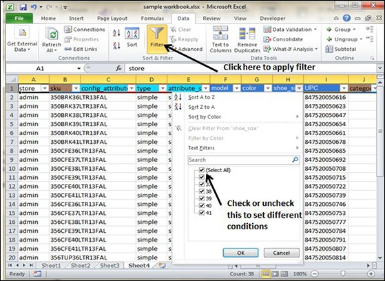
Click the drop-down arrow in the Area Row Header and remove the check mark from Select All, which unselects everything.
Then select the check mark for Size 36 which will filter the data and displays data of Shoe Size 36.
Some of the row numbers are missing; these rows contain the filtered (hidden) data.
There is drop-down arrow in the Area column now shows a different graphic — an icon that indicates the column is filtered.

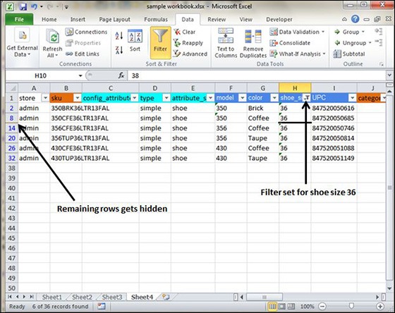
Using Multiple Filters

You can filter the records by multiple conditions i.e. by multiple column values. Suppose after size 36 is filtered, you need to have the filter where color is equal to Coffee. After setting filter for Shoe Size, choose Color column and then set filter for color.

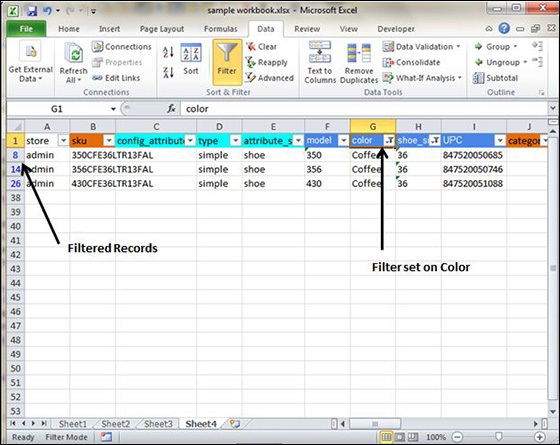
Data Sorting in Excel 2010

Sorting in MS Excel

Sorting data in MS Excel rearranges the rows based on the contents of a particular column. You may want to sort a table to put names in alphabetical order. Or, maybe you want to sort data by Amount from smallest to largest or largest to smallest.

To Sort the data follow the steps mentioned below.

Select the Column by which you want to sort data.
Choose Data Tab » Sort Below dialog appears.

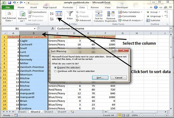
If you want to sort data based on a selected column, Choose Continue with the selection or if you want sorting based on other columns, choose Expand Selection.
You can Sort based on the below Conditions.
- Values − Alphabetically or numerically.
- Cell Color − Based on Color of Cell.
- Font Color − Based on Font color.
- Cell Icon − Based on Cell Icon.

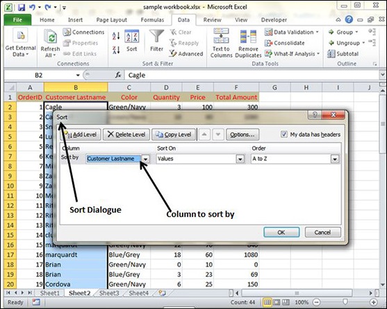
Clicking Ok will sort the data.

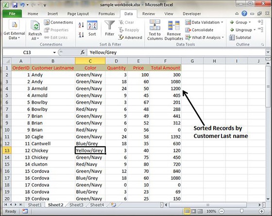
Sorting option is also available from the Home Tab. Choose Home Tab » Sort & Filter. You can see the same dialog to sort records.

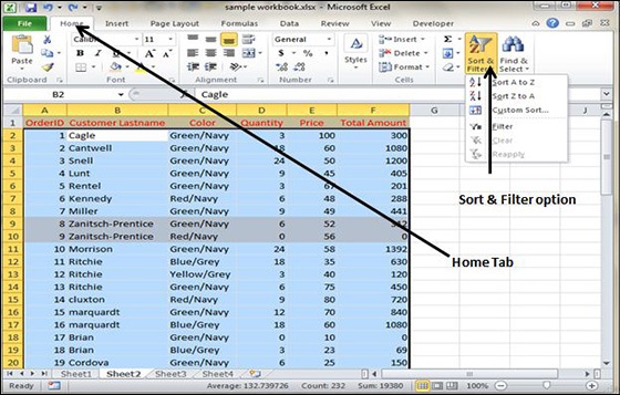
Using Ranges in Excel 2010

Ranges in MS Excel

A cell is a single element in a worksheet that can hold a value, some text, or a formula. A cell is identified by its address, which consists of its column letter and row number. For example, cell B1 is the cell in the second column and the first row.

A group of cells is called a range. You designate a range address by specifying its upper-left cell address and its lower-right cell address, separated by a colon.

Example of Ranges −

C24 − A range that consists of a single cell.
A1:B1 − Two cells that occupy one row and two columns.
A1:A100 − 100 cells in column A.
A1:D4 − 16 cells (four rows by four columns).

Selecting Ranges

You can select a range in several ways −

Press the left mouse button and drag, highlighting the range. Then release the mouse button. If you drag to the end of the screen, the worksheet will scroll.
Press the Shift key while you use the navigation keys to select a range.
Press F8 and then move the cell pointer with the navigation keys to highlight the range. Press F8 again to return the navigation keys to normal movement.
Type the cell or range address into the Name box and press Enter. Excel selects the cell or range that you specified.

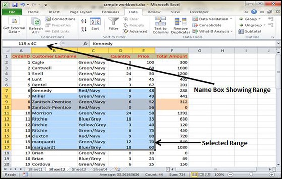
Selecting Complete Rows and Columns

When you need to select an entire row or column. You can select entire rows and columns in much the same manner as you select ranges −

Click the row or column border to select a single row or column.
To select multiple adjacent rows or columns, click a row or column border and drag to highlight additional rows or columns.
To select multiple (nonadjacent) rows or columns, press Ctrl while you click the row or column borders that you want.

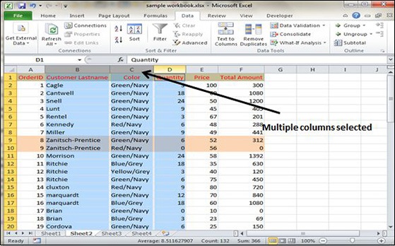
Data Validation in Excel 2010

Data Validation

MS Excel data validation feature allows you to set up certain rules that dictate what can be entered into a cell. For example, you may want to limit data entry in a particular cell to whole numbers between 0 and 10. If the user makes an invalid entry, you can display a custom message as shown below.

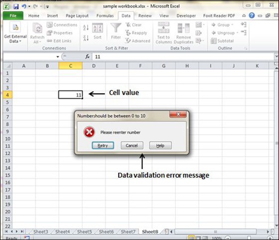
Validation Criteria

To specify the type of data allowable in a cell or range, follow the steps below, which shows all the three tabs of the Data Validation dialog box.

Select the cell or range.
Choose Data » Data Tools » Data Validation. Excel displays its Data Validation dialog box having 3 tabs settings, Input Message and Error alert.

Settings Tab

Here you can set the type of validation you need. Choose an option from the Allow drop-down list. The contents of the Data Validation dialog box will change, displaying controls based on your choice.

Any Value − Selecting this option removes any existing data validation.
Whole Number − The user must enter a whole number.For example, you can specify that the entry must be a whole number greater than or equal to 50.
Decimal − The user must enter a number. For example, you can specify that the entry must be greater than or equal to 10 and less than or equal to 20.
List − The user must choose from a list of entries you provide. You will create drop-down list with this validation. You have to give input ranges then those values will appear in the drop-down.
Date − The user must enter a date. You specify a valid date range from choices in the Data drop-down list. For example, you can specify that the entered data must be greater than or equal to January 1, 2013, and less than or equal to December 31, 2013.
Time − The user must enter a time. You specify a valid time range from choices in the Data drop-down list. For example, you can specify that the entered data must be later than 12:00 p.m.
Text Length − The length of the data (number of characters) is limited. You specify a valid length by using the Data drop-down list. For example, you can specify that the length of the entered data be 1 (a single alphanumeric character).
Custom − To use this option, you must supply a logical formula that determines the validity of the user’s entry (a logical formula returns either TRUE or FALSE).

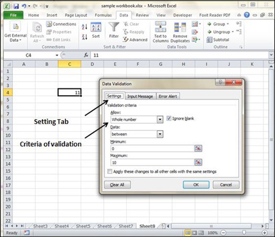
Input Message Tab

You can set the input help message with this tab. Fill the title and Input message of the Input message tab and the input message will appear when the cell is selected.

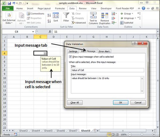
Error Alert Tab

You can specify an error message with this tab. Fill the title and error message. Select the style of the error as stop, warning or Information as per you need.

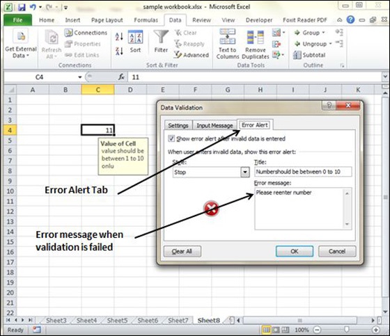
Using Styles in Excel 2010

Using Styles in MS Excel

With MS Excel 2010 Named styles make it very easy to apply a set of predefined formatting options to a cell or range. It saves time as well as make sure that look of the cells are consistent.

A Style can consist of settings for up to six different attributes −

Number format
Font (type, size, and color)
Alignment (vertical and horizontal)
Borders
Pattern
Protection (locked and hidden)

Now, let us see how styles are helpful. Suppose that you apply a particular style to some twenty cells scattered throughout your worksheet. Later, you realize that these cells should have a font size of 12 pt. rather than 14 pt. Rather than changing each cell, simply edit the style. All cells with that particular style change automatically.

Applying Styles

Choose Home » Styles » Cell Styles. Note that this display is a live preview, that is, as you move your mouse over the style choices, the selected cell or range temporarily displays the style. When you see a style you like, click it to apply the style to the selection.

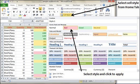
Creating Custom Style in MS Excel

We can create new custom style in Excel 2010. To create a new style, follow these steps −

Select a cell and click on Cell styles from Home Tab.
Click on New Cell Style and give style name.
Click on Format to apply formatting to the cell.

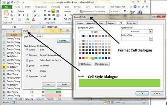
After applying formatting click on OK. This will add new style in the styles. You can view it on Home » Styles.

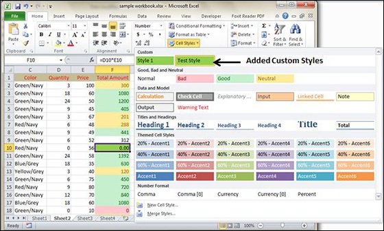
Using Themes in Excel 2010

Using Themes in MS Excel

To help users create more professional-looking documents, MS Excel has incorporated a concept known as document themes. By using themes, it is easy to specify the colors, fonts, and a variety of graphic effects in a document. And best of all, changing the entire look of your document is a breeze. A few mouse clicks is all it takes to apply a different theme and change the look of your workbook.

Applying Themes

Choose Page layout Tab » Themes Dropdown. Note that this display is a live preview, that is, as you move your mouse over the Theme, it temporarily displays the theme effect. When you see a style you like, click it to apply the style to the selection.

Creating Custom Theme in MS Excel

We can create new custom Theme in Excel 2010. To create a new style, follow these steps −

Click on the save current theme option under Theme in Page Layout Tab.
This will save the current theme to office folder.
You can browse the theme later to load the theme.

Using Templates in Excel 2010

Using Templates in MS Excel

Template is essentially a model that serves as the basis for something. An Excel template is a workbook that’s used to create other workbooks.

Viewing Available Templates

To view the Excel templates, choose File » New to display the available templates screen in Backstage View. You can select a template stored on your hard drive, or a template from Microsoft Office Online. If you choose a template from Microsoft Office Online, you must be connected to the Internet to download it. The Office Online Templates section contains a number of icons, which represents various categories of templates. Click an icon, and you’ll see the available templates. When you select a template thumbnail, you can see a preview in the right panel.

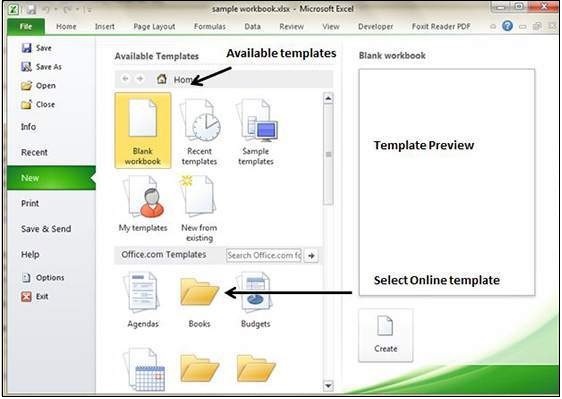
On-line Templates

These template data is available online at the Microsoft server. When you select the template and click on it, it will download the template data from Microsoft server and opens it as shown below.

Using Templates in MS Excel

Template is essentially a model that serves as the basis for something. An Excel template is a workbook that’s used to create other workbooks.

Viewing Available Templates

On-line Templates

These template data is available online at the Microsoft server. When you select the template and click on it, it will download the template data from Microsoft server and opens it as shown below.

Using Macros in Excel 2010

Macros in MS Excel

Macros enable you to automate almost any task that you can undertake in Excel 2010. By using macro recorder from View Tab » Macro Dropdown to record tasks that you perform routinely, you not only speed up the procedure considerably but you are assured that each step in a task is carried out the same way each and every time you perform a task.

To view macros choose View Tab » Macro dropdown.

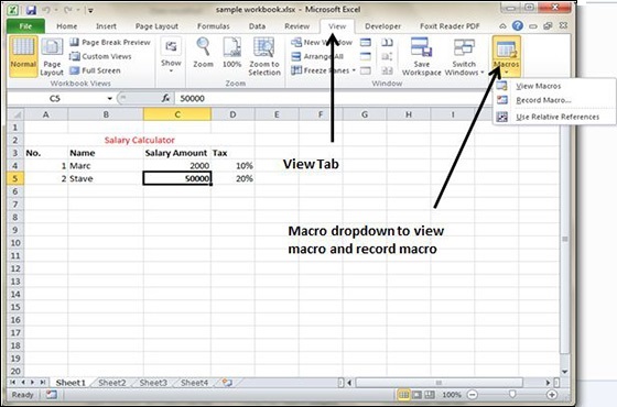
Macro Options

View tab contains a Macros command button to which a dropdown menu containing the following three options.

View Macros − Opens the Macro dialog box where you can select a macro to run or edit.
Record Macro − Opens the Record Macro dialog box where you define the settings for your new macro and then start the macro recorder; this is the same as clicking the Record Macro button on the Status bar.
Use Relative References − Uses relative cell addresses when recording a macro, making the macro more versatile by enabling you to run it in areas of a worksheet other than the ones originally used in the macro’s recording.

Creating Macros

You can create macros in one of two ways −

Use MS Excel’s macro recorder to record your actions as you undertake them in a worksheet.
Enter the instructions that you want to be followed in a VBA code in the Visual Basic Editor.

Now let’s create a simple macro that will automate the task of making cell content Bold and apply cell color.

Choose View Tab » Macro dropdown.
Click on Record Macro as below.

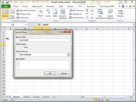
Now Macro recording will start.
Do the steps of action, which you want to perform repeatedly. Macro will record those steps.
You can stop the macro recording once done with all steps.

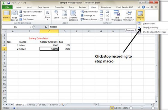
Edit Macro

You can edit the created Macro at any time. Editing macro will take you to the VBA programming editor.

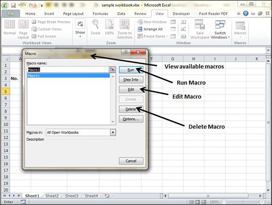
Adding Graphics in Excel 2010

Graphic Objects in MS Excel

MS Excel supports various types of graphic objects like Shapes gallery, SmartArt, Text Box, and WordArt available on the Insert tab of the Ribbon.Graphics are available in the Insert Tab. See the screenshots below for various available graphics in MS Excel 2010.

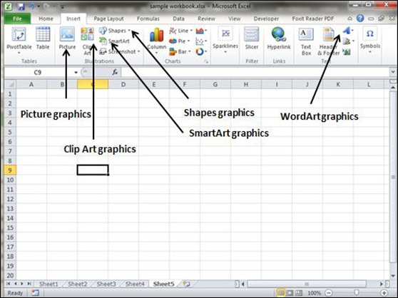
Insert Shape

Choose Insert Tab » Shapes dropdown.
Select the shape you want to insert. Click on shape to insert it.
To edit the inserted shape just drag the shape with the mouse. Shape will adjust the shape.

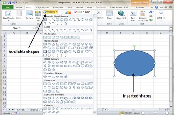
Insert Smart Art

Choose Insert Tab » SmartArt.
Clicking SmartArt will open the SmartArt dialogue as shown below in the screen-shot. Choose from the list of available smartArts.
Click on SmartArt to Insert it in the worksheet.
Edit the SmartArt as per your need.

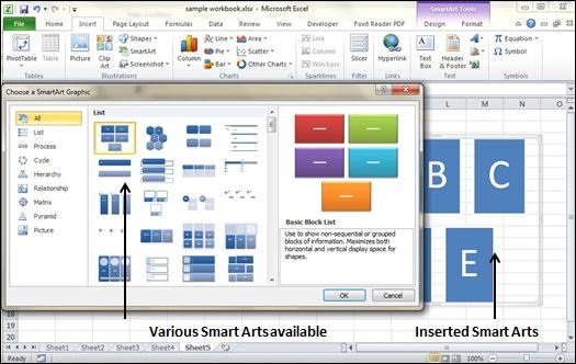
Insert Clip Art

Choose Insert Tab » Clip Art.
Clicking Clip Art will open the search box as shown in the below screen-shot. Choose from the list of available Clip Arts.
Click on Clip Art to Insert it in the worksheet.

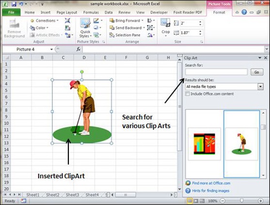
Insert Word Art

Choose Insert Tab » WordArt.
Select the style of WordArt, which you like and click it to enter a text in it.

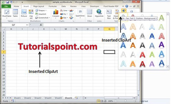
Cross Referencing in Excel 2010

Graphic Objects in MS Excel

When you have information spread across several different spreadsheets, it can seem a daunting task to bring all these different sets of data together into one meaningful list or table. This is where the Vlookup function comes into its own.

VLOOKUP

VlookUp searches for a value vertically down for the lookup table. VLOOKUP(lookup_value,table_array,col_index_num,range_lookup) has 4 parameters as below.

lookup_value − It is the user input. This is the value that the function uses to search on.
The table_array − It is the area of cells in which the table is located. This includes not only the column being searched on, but the data columns for which you are going to get the values that you need.
Col_index_num − It is the column of data that contains the answer that you want.
Range_lookup − It is a TRUE or FALSE value. When set to TRUE, the lookup function gives the closest match to the lookup_value without going over the lookup_value. When set to FALSE, an exact match must be found to the lookup_value or the function will return #N/A. Note, this requires that the column containing the lookup_value be formatted in ascending order.

VLOOKUP Example

Let’s look at a very simple example of cross-referencing two spreadsheets. Each spreadsheet contains information about the same group of people. The first spreadsheet has their dates of birth, and the second shows their favorite color. How do we build a list showing the person’s name, their date of birth and their favorite color? VLOOOKUP will help in this case. First of all, let us see data in both the sheets.

This is data in the first sheet

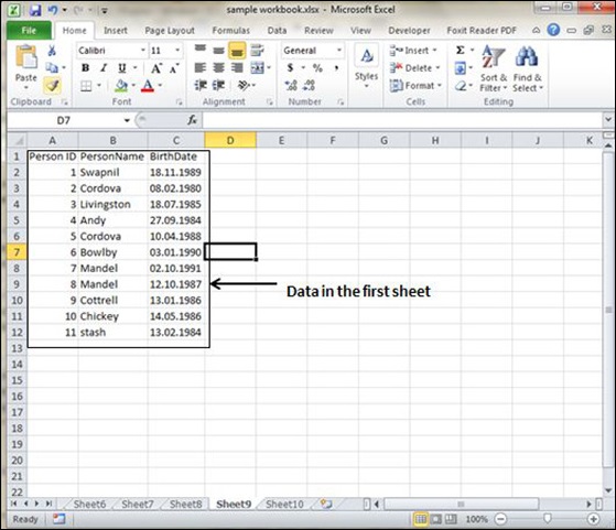
This is data in the second sheet

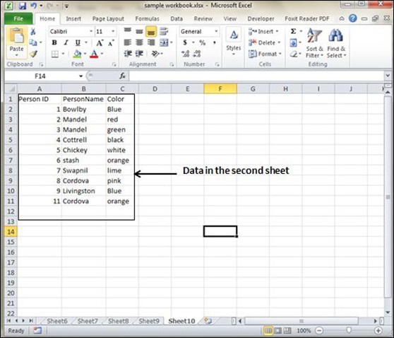
Now for finding the respective favorite color for that person from another sheet we need to vlookup the data. First argument to the VLOOKUP is lookup value (In this case it is person name). Second argument is the table array, which is table in the second sheet from B2 to C11. Third argument to VLOOKUP is Column index num, which is the answer we are looking for. In this case, it is 2 the color column number is 2. The fourth argument is True returning partial match or false returning exact match. After applying VLOOKUP formula it will calculate the color and the results are displayed as below.

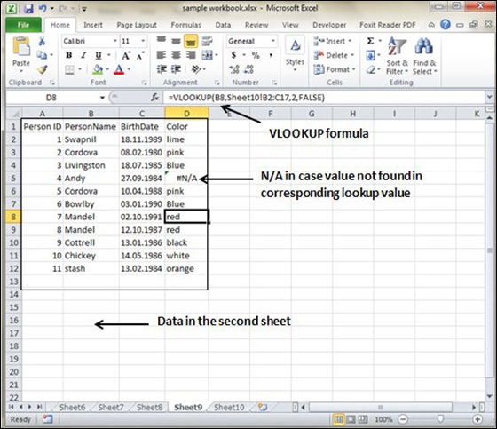
As you can see in the above screen-shot that results of VLOOKUP has searched for color in the second sheet table. It has returned #N/A in case where match is not found. In this case, Andy’s data is not present in the second sheet so it returned #N/A.

Printing Worksheets in Excel 2010

Quick Print

If you want to print a copy of a worksheet with no layout adjustment, use the Quick Print option. There are two ways in which we can use this option.

Choose File » Print (which displays the Print pane), and then click the Print button.
Press Ctrl+P and then click the Print button (or press Enter).

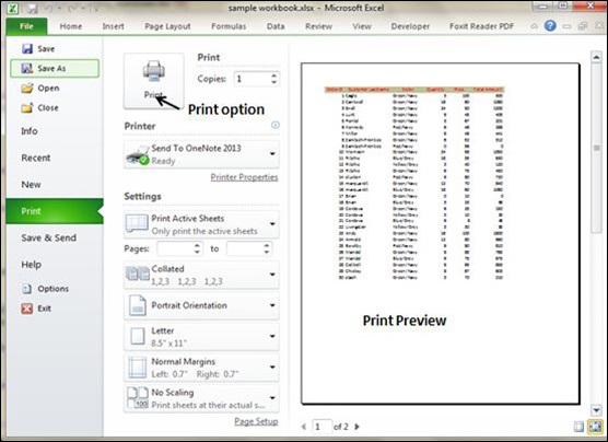
Adjusting Common Page Setup Settings

You can adjust the print settings available in the Page setup dialogue in different ways as discussed below. Page setup options include Page orientation, Page Size, Page Margins, etc.

The Print screen in Backstage View, displayed when you choose File » Print.
The Page Layout tab of the Ribbon.

Choosing Your Printer

To switch to a different printer, choose File » Print and use the drop-down control in the Printer section to select any other installed printer.

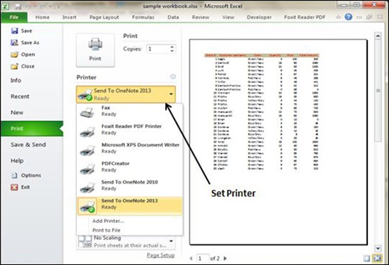
Specifying What You Want to Print

Sometimes you may want to print only a part of the worksheet rather than the entire active area. Choose File » Print and use the controls in the Settings section to specify what to print.

Active Sheets − Prints the active sheet or sheets that you selected.
Entire Workbook − Prints the entire workbook, including chart sheets.
Selection − Prints only the range that you selected before choosing File » Print.

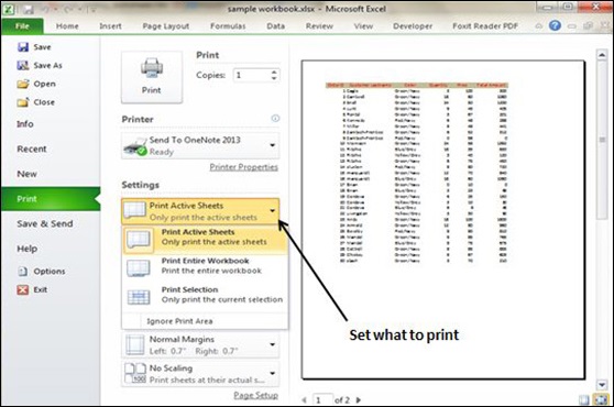
Email Workbooks MS Excel 2010

Email Workbook

MS Excel allows you to email the workbook very easily. To email the workbook to anyone, follow the below mentioned steps.

Choose File » Save and Send. It basically saves the document first and then the emails.

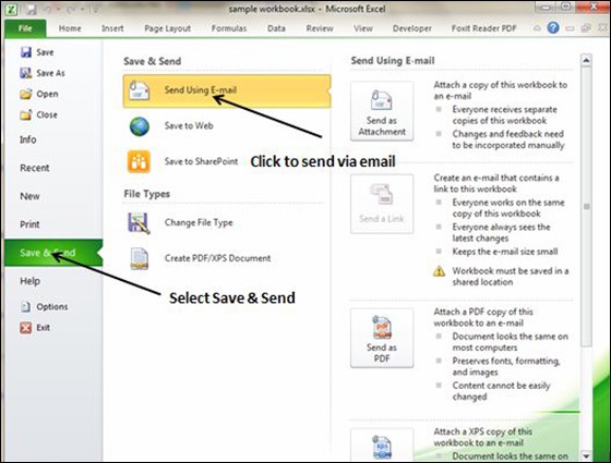
Click on Send using E-mail if your email system is configured. MS Outlook will open with the file as attachment in the New Email Window. You can send mail this workbook to anyone with valid email address.

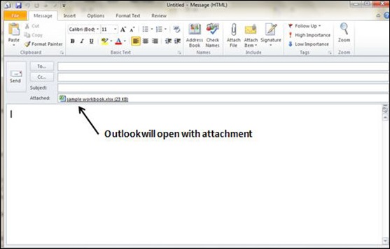
Translate Worksheet in Excel 2010

Translate Worksheet

You can translate the text written in a different language, such as phrases or paragraphs, individual words (by using the Mini Translator), or translate your whole file with MS Excel 2010.

Translation is available in the review tab of the ribbon in MS Excel 2010. You can quickly translate cell into different language with this option.

Performing Translation Step By Step

Select the content, which you want to translate to a different language.
Choose review tab » translation.
It will open the pane from which you can select the language to which you need to translate.
You need to have an internet connection for performing translation. It will translate using the Microsoft Translator.
Click on Insert to apply translation changes.

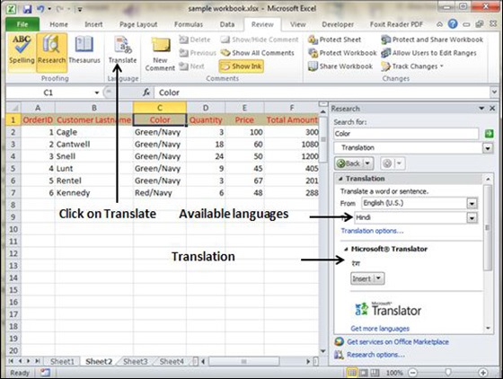
Workbook Security in Excel 2010

Workbook Security

We can apply security to the workbook by the concept of protection available in the Review Tab of ribbon. MS Excel’s protection-related features fall into three categories.

Worksheet protection − Protecting a worksheet from being modified, or restricting the modifications to certain users.
Workbook protection − Protecting a workbook from having sheets inserted or deleted, and also requiring the use of password to open the workbook.

Protect Worksheet

You may want to protect a worksheet for a variety of reasons. One reason is to prevent yourself or others from accidentally deleting the formulas or other critical data. A common scenario is to protect a worksheet, so that the data can be changed, but the formulas can’t be changed.

To protect a worksheet, choose Review » Changes group » Protect Sheet. Excel displays the Protect Sheet dialog box. Note that providing a password is optional. If you enter a password, that password will be required to unprotect the worksheet. You can select various options in which the sheet should be protected. Suppose we checked Format Cells option then Excel will not allow to format cells.

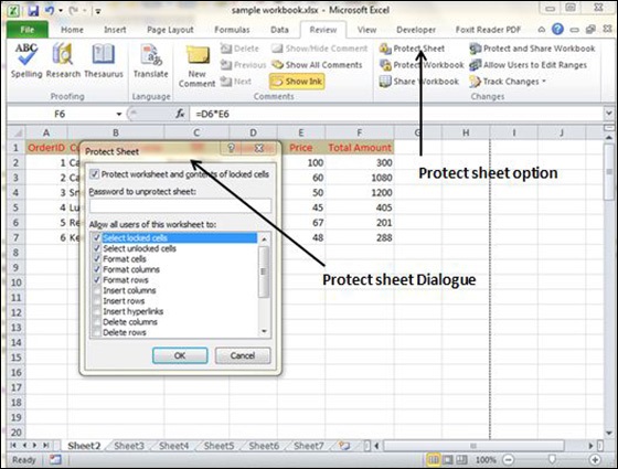
When somebody tries to format the cells, he or she will get the error as shown in the screenshot below.

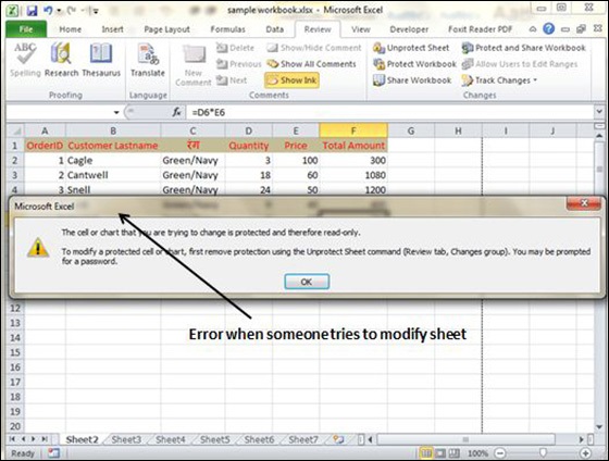
To unprotect a protected sheet, choose Review » Changes group » Unprotect Sheet. If the sheet was protected with a password, you’re prompted to enter that password.

Protecting a Workbook

Excel provides three ways to protect a workbook.

Requires a password to open the workbook.
Prevents the users from adding sheets, deleting sheets, hiding sheets, and unhiding sheets.
Prevents users from changing the size or position of windows.

Requiring a Password to Open a Workbook

Excel lets you save a workbook with a password. After doing so, whoever tries to open the workbook, must enter the password. To add a password to a workbook, follow these steps.

Choose File » Info » Protect Workbook » Encrypt With Password. Excel displays the Encrypt Document dialog box.
Type a password and click OK.
Type the password again and click OK.
Save the workbook.

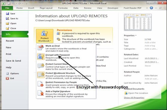
To remove a password from a workbook, repeat the same procedure. In Step 2, however, delete the existing password symbols.

Protecting Workbook’s Structure and Windows

To prevent others (or yourself) from performing certain actions in a workbook, you can protect the workbook’s structure and windows. When a workbook’s structure and windows are protected, the user may not Add a sheet, Delete a sheet, Hide a sheet, unhide a sheet, etc., and may not be allowed to change the size or position of a workbook’s windows respectively.

To protect a worksheet’s structure and windows, follow the below mentioned steps.

Choose Review » Changes group » Protect Workbook to display the Protect Workbook dialog box.
In the Protect Workbook dialog box, select the Structure check box and Windows check box.
(Optional) Enter a password.
Click OK.

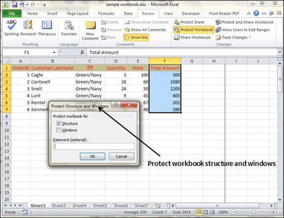
Data Tables in Excel 2010

Data Tables

In Excel, a Data Table is a way to see different results by altering an input cell in your formula. Data tables are available in Data Tab » What-If analysis dropdown » Data table in MS Excel.

Data Table with Example

Now, let us see data table concept with an example. Suppose you have the Price and quantity of many values. Also, you have the discount for that as third variable for calculating the Net Price. You can keep the Net Price value in the organized table format with the help of the data table. Your Price runs horizontally to the right while quantity runs vertically down. We are using a formula to calculate the Net Price as Price multiplied by Quantity minus total discount (Quantity * Discount for each quantity).

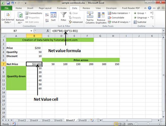
Now, for creation of data table select the range of data table. Choose Data Tab » What-If analysis dropdown » Data table. It will give you dialogue asking for Input row and Input Column. Give the Input row as Price cell (In this case cell B3) and Input column as quantity cell (In this case cell B4). Please see the below screen-shot.

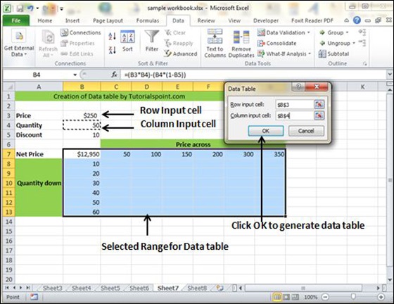
Clicking OK will generate data table as shown in the below screen-shot. It will generate the table formula. You can change the price horizontally or quantity vertically to see the change in the Net Price.

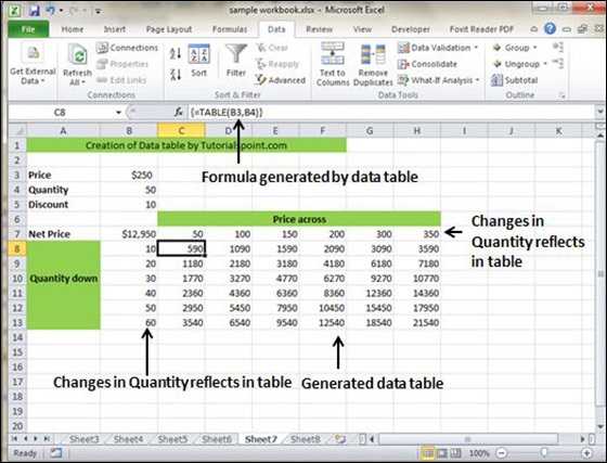
Pivot Tables in Excel 2010

Pivot Tables

A pivot table is essentially a dynamic summary report generated from a database. The database can reside in a worksheet (in the form of a table) or in an external data file. A pivot table can help transform endless rows and columns of numbers into a meaningful presentation of the data. Pivot tables are very powerful tool for summarized analysis of the data.

Pivot tables are available under Insert tab » PivotTable dropdown » PivotTable.

Pivot Table Example

Now, let us see Pivot table with the help of example. Suppose you have huge data of voters and you want to see the summarized data of voter Information per party, then you can use the Pivot table for it. Choose Insert tab » Pivot Table to insert pivot table. MS Excel selects the data of the table. You can select the pivot table location as existing sheet or new sheet.

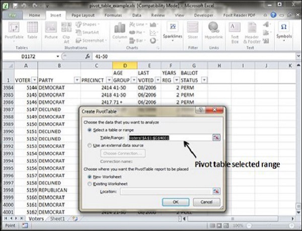
This will generate the Pivot table pane as shown below. You have various options available in the Pivot table pane. You can select fields for the generated pivot table.

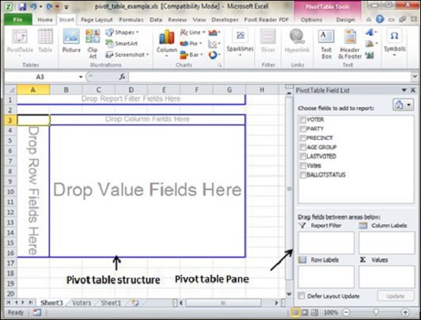
Column labels − A field that has a column orientation in the pivot table. Each item in the field occupies a column.
Report Filter − You can set the filter for the report as year, then data gets filtered as per the year.
Row labels − A field that has a row orientation in the pivot table. Each item in the field occupies a row.
Values area − The cells in a pivot table that contain the summary data. Excel offers several ways to summarize the data (sum, average, count, and so on).

After giving input fields to the pivot table, it generates the pivot table with the data as shown below.

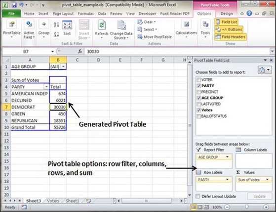
Simple Charts in Excel 2010

Charts

A chart is a visual representation of numeric values. Charts (also known as graphs) have been an integral part of spreadsheets. Charts generated by early spreadsheet products were quite crude, but thy have improved significantly over the years. Excel provides you with the tools to create a wide variety of highly customizable charts. Displaying data in a well-conceived chart can make your numbers more understandable. Because a chart presents a picture, charts are particularly useful for summarizing a series of numbers and their interrelationships.

Types of Charts

There are various chart types available in MS Excel as shown in the below screen-shot.

Charts

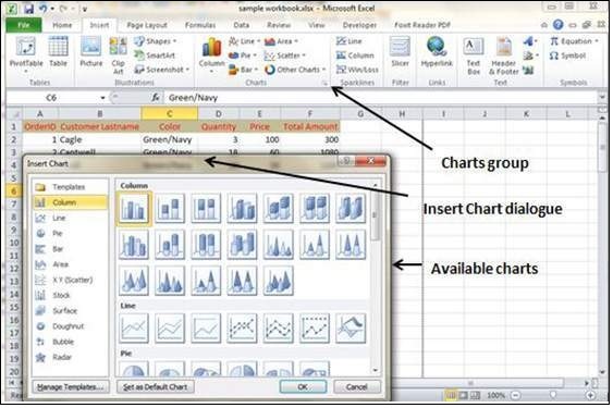
Column − Column chart shows data changes over a period of time or illustrates comparisons among items.
Bar − A bar chart illustrates comparisons among individual items.
Pie − A pie chart shows the size of items that make up a data series, proportional to the sum of the items. It always shows only one data series and is useful when you want to emphasize a significant element in the data.
Line − A line chart shows trends in data at equal intervals.
Area − An area chart emphasizes the magnitude of change over time.
X Y Scatter − An xy (scatter) chart shows the relationships among the numeric values in several data series, or plots two groups of numbers as one series of xy coordinates.
Stock − This chart type is most often used for stock price data, but can also be used for scientific data (for example, to indicate temperature changes).
Surface − A surface chart is useful when you want to find the optimum combinations between two sets of data. As in a topographic map, colors and patterns indicate areas that are in the same range of values.
Doughnut − Like a pie chart, a doughnut chart shows the relationship of parts to a whole; however, it can contain more than one data series.
Bubble − Data that is arranged in columns on a worksheet, so that x values are listed in the first column and corresponding y values and bubble size values are listed in adjacent columns, can be plotted in a bubble chart.
Radar − A radar chart compares the aggregate values of a number of data series.

Creating Chart

To create charts for the data by below mentioned steps.

Select the data for which you want to create the chart.
Choose Insert Tab » Select the chart or click on the Chart group to see various chart types.
Select the chart of your choice and click OK to generate the chart.

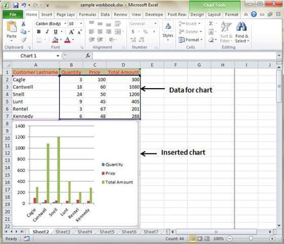
Editing Chart

You can edit the chart at any time after you have created it.

You can select the different data for chart input with Right click on chart » Select data. Selecting new data will generate the chart as per the new data, as shown in the below screen-shot.

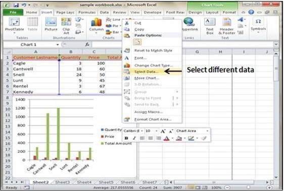
You can change the X axis of the chart by giving different inputs to X-axis of chart.
You can change the Y axis of chart by giving different inputs to Y-axis of chart.

Pivot Charts Excel 2010

Pivot Charts

A pivot chart is a graphical representation of a data summary, displayed in a pivot table. A pivot chart is always based on a pivot table. Although Excel lets you create a pivot table and a pivot chart at the same time, you can’t create a pivot chart without a pivot table. All Excel charting features are available in a pivot chart.

Pivot charts are available under Insert tab » PivotTable dropdown » PivotChart.

Pivot Chart Example

Now, let us see Pivot table with the help of an example. Suppose you have huge data of voters and you want to see the summarized view of the data of voter Information per party in the form of charts, then you can use the Pivot chart for it. Choose Insert tab » Pivot Chart to insert the pivot table.

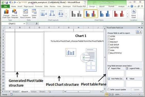
MS Excel selects the data of the table. You can select the pivot chart location as an existing sheet or a new sheet. Pivot chart depends on automatically created pivot table by the MS Excel. You can generate the pivot chart in the below screen-shot.

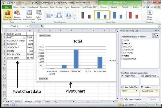
Keyboard Shortcuts in Excel 2010

MS Excel Keyboard Short-cuts

MS Excel offers many keyboard short-cuts. If you are familiar with windows operating system, you should be aware of most of them. Below is the list of all the major shortcut keys in Microsoft Excel.

Ctrl + A − Selects all contents of the worksheet.
Ctrl + B − Bold highlighted selection.
Ctrl + I − Italicizes the highlighted selection.
Ctrl + K − Inserts link.
Ctrl + U − Underlines the highlighted selection.
Ctrl + 1 − Changes the format of selected cells.
Ctrl + 5 − Strikethrough the highlighted selection.
Ctrl + P − Brings up the print dialog box to begin printing.
Ctrl + Z − Undo last action.
Ctrl + F3 − Opens Excel Name Manager.
Ctrl + F9 − Minimizes the current window.
Ctrl + F10 − Maximize currently selected window.
Ctrl + F6 − Switches between open workbooks or windows.
Ctrl + Page up − Moves between Excel work sheets in the same Excel document.
Ctrl + Page down − Moves between Excel work sheets in the same Excel document.
Ctrl + Tab − Moves between Two or more open Excel files.
Alt + = − Creates a formula to sum all of the above cells
Ctrl + ‘ − Inserts the value of the above cell into cell currently selected.
Ctrl + Shift + ! − Formats the number in comma format.
Ctrl + Shift + $ − Formats the number in currency format.
Ctrl + Shift + # − Formats the number in date format.
Ctrl + Shift + % − Formats the number in percentage format.
Ctrl + Shift + ^ − Formats the number in scientific format.
Ctrl + Shift + @ − Formats the number in time format.
Ctrl + Arrow key − Moves to the next section of text.
Ctrl + Space − Selects the entire column.
Shift + Space − Selects the entire row.
Ctrl + — − Deletes the selected column or row.
Ctrl + Shift + = − Inserts a new column or row.
Ctrl + Home − Moves to cell A1.
Ctrl + ~ − Switches between showing Excel formulas or their values in cells.
F2 − Edits the selected cell.
F3 − After a name has been created F3 will paste names.
F4 − Repeat last action. For example, if you changed the color of text in another cell pressing F4 will change the text in cell to the same color.
F5 − Goes to a specific cell. For example, C6.
F7 − Spell checks the selected text or document.
F11 − Creates chart from the selected data.
Ctrl + Shift + ; − Enters the current time.
Ctrl + ; − Enters the current date.
Alt + Shift + F1 − Inserts New Worksheet.
Alt + Enter − While typing text in a cell pressing Alt + Enter will move to the next line allowing for multiple lines of text in one cell.
Shift + F3 − Opens the Excel formula window.
Shift + F5 − Brings up the search box.

Источник