
Split text into different columns with functions
Excel for Microsoft 365 Excel for Microsoft 365 for Mac Excel for the web Excel 2021 Excel 2021 for Mac Excel 2019 Excel 2019 for Mac Excel 2016 Excel 2016 for Mac Excel 2013 Excel Web App Excel 2010 Excel 2007 Excel for Mac 2011 More…Less
You can use the LEFT, MID, RIGHT, SEARCH, and LEN text functions to manipulate strings of text in your data. For example, you can distribute the first, middle, and last names from a single cell into three separate columns.
The key to distributing name components with text functions is the position of each character within a text string. The positions of the spaces within the text string are also important because they indicate the beginning or end of name components in a string.
For example, in a cell that contains only a first and last name, the last name begins after the first instance of a space. Some names in your list may contain a middle name, in which case, the last name begins after the second instance of a space.
This article shows you how to extract various components from a variety of name formats using these handy functions. You can also split text into different columns with the Convert Text to Columns Wizard
|
Example name |
Description |
First name |
Middle name |
Last name |
Suffix |
|
|
1 |
Jeff Smith |
No middle name |
Jeff |
Smith |
||
|
2 |
Eric S. Kurjan |
One middle initial |
Eric |
S. |
Kurjan |
|
|
3 |
Janaina B. G. Bueno |
Two middle initials |
Janaina |
B. G. |
Bueno |
|
|
4 |
Kahn, Wendy Beth |
Last name first, with comma |
Wendy |
Beth |
Kahn |
|
|
5 |
Mary Kay D. Andersen |
Two-part first name |
Mary Kay |
D. |
Andersen |
|
|
6 |
Paula Barreto de Mattos |
Three-part last name |
Paula |
Barreto de Mattos |
||
|
7 |
James van Eaton |
Two-part last name |
James |
van Eaton |
||
|
8 |
Bacon Jr., Dan K. |
Last name and suffix first, with comma |
Dan |
K. |
Bacon |
Jr. |
|
9 |
Gary Altman III |
With suffix |
Gary |
Altman |
III |
|
|
10 |
Mr. Ryan Ihrig |
With prefix |
Ryan |
Ihrig |
||
|
11 |
Julie Taft-Rider |
Hyphenated last name |
Julie |
Taft-Rider |
Note: In the graphics in the following examples, the highlight in the full name shows the character that the matching SEARCH formula is looking for.
This example separates two components: first name and last name. A single space separates the two names.
Copy the cells in the table and paste into an Excel worksheet at cell A1. The formula you see on the left will be displayed for reference, while Excel will automatically convert the formula on the right into the appropriate result.
Hint Before you paste the data into the worksheet, set the column widths of columns A and B to 250.
|
Example name |
Description |
|
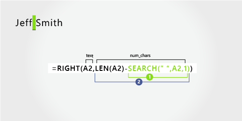
Jeff Smith |
No middle name |
|
Formula |
Result (first name) |
|
‘=LEFT(A2, SEARCH(» «,A2,1)) |
=LEFT(A2, SEARCH(» «,A2,1)) |
|
Formula |
Result (last name) |
|
‘=RIGHT(A2,LEN(A2)-SEARCH(» «,A2,1)) |
=RIGHT(A2,LEN(A2)-SEARCH(» «,A2,1)) |
-
First name
The first name starts with the first character in the string (J) and ends at the fifth character (the space). The formula returns five characters in cell A2, starting from the left.

Use the SEARCH function to find the value for num_chars:
Search for the numeric position of the space in A2, starting from the left.
-
Last name
The last name starts at the space, five characters from the right, and ends at the last character on the right (h). The formula extracts five characters in A2, starting from the right.
Use the SEARCH and LEN functions to find the value for num_chars:
Search for the numeric position of the space in A2, starting from the left. (5)
-
Count the total length of the text string, and then subtract the number of characters to the left of the first space, as found in step 1.

This example uses a first name, middle initial, and last name. A space separates each name component.
Copy the cells in the table and paste into an Excel worksheet at cell A1. The formula you see on the left will be displayed for reference, while Excel will automatically convert the formula on the right into the appropriate result.
Hint Before you paste the data into the worksheet, set the column widths of columns A and B to 250.
|
Example name |
Description |
|
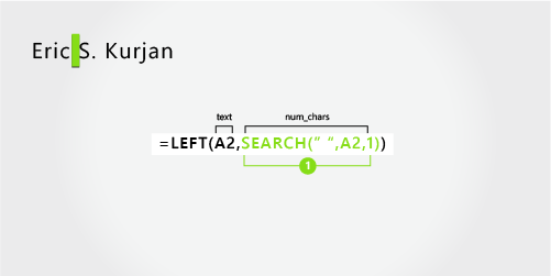
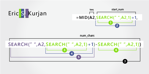
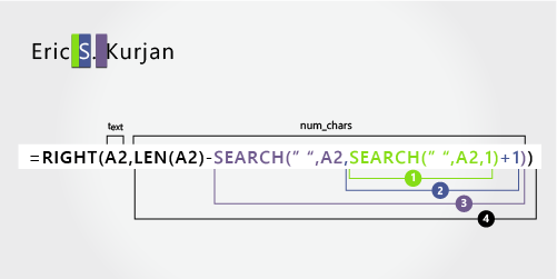
Eric S. Kurjan |
One middle initial |
|
Formula |
Result (first name) |
|
‘=LEFT(A2, SEARCH(» «,A2,1)) |
=LEFT(A2, SEARCH(» «,A2,1)) |
|
Formula |
Result (middle initial) |
|
‘=MID(A2,SEARCH(» «,A2,1)+1,SEARCH(» «,A2,SEARCH(» «,A2,1)+1)-SEARCH(» «,A2,1)) |
=MID(A2,SEARCH(» «,A2,1)+1,SEARCH(» «,A2,SEARCH(» «,A2,1)+1)-SEARCH(» «,A2,1)) |
|
Formula |
Live Result (last name) |
|
‘=RIGHT(A2,LEN(A2)-SEARCH(» «,A2,SEARCH(» «,A2,1)+1)) |
=RIGHT(A2,LEN(A2)-SEARCH(» «,A2,SEARCH(» «,A2,1)+1)) |
-
First name
The first name starts with the first character from the left (E) and ends at the fifth character (the first space). The formula extracts the first five characters in A2, starting from the left.
Use the SEARCH function to find the value for num_chars:
Search for the numeric position of the space in A2, starting from the left. (5)
-
Middle name
The middle name starts at the sixth character position (S), and ends at the eighth position (the second space). This formula involves nesting SEARCH functions to find the second instance of a space.
The formula extracts three characters, starting from the sixth position.
Use the SEARCH function to find the value for start_num:
Search for the numeric position of the first space in A2, starting from the first character from the left. (5).
-
Add 1 to get the position of the character after the first space (S). This numeric position is the starting position of the middle name. (5 + 1 = 6)
Use nested SEARCH functions to find the value for num_chars:
Search for the numeric position of the first space in A2, starting from the first character from the left. (5)
-
Add 1 to get the position of the character after the first space (S). The result is the character number at which you want to start searching for the second instance of space. (5 + 1 = 6)
-
Search for the second instance of space in A2, starting from the sixth position (S) found in step 4. This character number is the ending position of the middle name. (8)
-
Search for the numeric position of space in A2, starting from the first character from the left. (5)
-
Take the character number of the second space found in step 5 and subtract the character number of the first space found in step 6. The result is the number of characters MID extracts from the text string starting at the sixth position found in step 2. (8 – 5 = 3)
-
Last name
The last name starts six characters from the right (K) and ends at the first character from the right (n). This formula involves nesting SEARCH functions to find the second and third instances of a space (which are at the fifth and eighth positions from the left).
The formula extracts six characters in A2, starting from the right.
-
Use the LEN and nested SEARCH functions to find the value for num_chars:
Search for the numeric position of space in A2, starting from the first character from the left. (5)
-
Add 1 to get the position of the character after the first space (S). The result is the character number at which you want to start searching for the second instance of space. (5 + 1 = 6)
-
Search for the second instance of space in A2, starting from the sixth position (S) found in step 2. This character number is the ending position of the middle name. (8)
-
Count the total length of the text string in A2, and then subtract the number of characters from the left up to the second instance of space found in step 3. The result is the number of characters to be extracted from the right of the full name. (14 – 8 = 6).
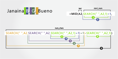
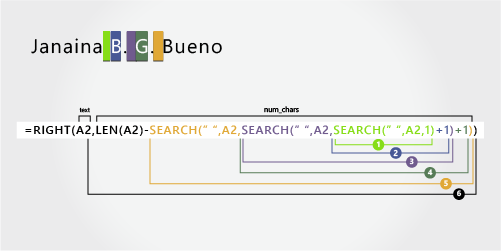
Here’s an example of how to extract two middle initials. The first and third instances of space separate the name components.
Copy the cells in the table and paste into an Excel worksheet at cell A1. The formula you see on the left will be displayed for reference, while Excel will automatically convert the formula on the right into the appropriate result.
Hint Before you paste the data into the worksheet, set the column widths of columns A and B to 250.
|
Example name |
Description |
|
Janaina B. G. Bueno |
Two middle initials |
|
Formula |
Result (first name) |
|
‘=LEFT(A2, SEARCH(» «,A2,1)) |
=LEFT(A2, SEARCH(» «,A2,1)) |
|
Formula |
Result (middle initials) |
|
‘=MID(A2,SEARCH(» «,A2,1)+1,SEARCH(» «,A2,SEARCH(» «,A2,SEARCH(» «,A2,1)+1)+1)-SEARCH(» «,A2,1)) |
=MID(A2,SEARCH(» «,A2,1)+1,SEARCH(» «,A2,SEARCH(» «,A2,SEARCH(» «,A2,1)+1)+1)-SEARCH(» «,A2,1)) |
|
Formula |
Live Result (last name) |
|
‘=RIGHT(A2,LEN(A2)-SEARCH(» «,A2,SEARCH(» «,A2,SEARCH(» «,A2,1)+1)+1)) |
=RIGHT(A2,LEN(A2)-SEARCH(» «,A2,SEARCH(» «,A2,SEARCH(» «,A2,1)+1)+1)) |
-
First name
The first name starts with the first character from the left (J) and ends at the eighth character (the first space). The formula extracts the first eight characters in A2, starting from the left.
Use the SEARCH function to find the value for num_chars:
Search for the numeric position of the first space in A2, starting from the left. (8)
-
Middle name
The middle name starts at the ninth position (B), and ends at the fourteenth position (the third space). This formula involves nesting SEARCH to find the first, second, and third instances of space in the eighth, eleventh, and fourteenth positions.
The formula extracts five characters, starting from the ninth position.
Use the SEARCH function to find the value for start_num:
Search for the numeric position of the first space in A2, starting from the first character from the left. (8)
-
Add 1 to get the position of the character after the first space (B). This numeric position is the starting position of the middle name. (8 + 1 = 9)
Use nested SEARCH functions to find the value for num_chars:
Search for the numeric position of the first space in A2, starting from the first character from the left. (8)
-
Add 1 to get the position of the character after the first space (B). The result is the character number at which you want to start searching for the second instance of space. (8 + 1 = 9)
-
Search for the second space in A2, starting from the ninth position (B) found in step 4. (11).
-
Add 1 to get the position of the character after the second space (G). This character number is the starting position at which you want to start searching for the third space. (11 + 1 = 12)
-
Search for the third space in A2, starting at the twelfth position found in step 6. (14)
-
Search for the numeric position of the first space in A2. (8)
-
Take the character number of the third space found in step 7 and subtract the character number of the first space found in step 6. The result is the number of characters MID extracts from the text string starting at the ninth position found in step 2.
-
Last name
The last name starts five characters from the right (B) and ends at the first character from the right (o). This formula involves nesting SEARCH to find the first, second, and third instances of space.
The formula extracts five characters in A2, starting from the right of the full name.
Use nested SEARCH and the LEN functions to find the value for the num_chars:
Search for the numeric position of the first space in A2, starting from the first character from the left. (8)
-
Add 1 to get the position of the character after the first space (B). The result is the character number at which you want to start searching for the second instance of space. (8 + 1 = 9)
-
Search for the second space in A2, starting from the ninth position (B) found in step 2. (11)
-
Add 1 to get the position of the character after the second space (G). This character number is the starting position at which you want to start searching for the third instance of space. (11 + 1 = 12)
-
Search for the third space in A2, starting at the twelfth position (G) found in step 6. (14)
-
Count the total length of the text string in A2, and then subtract the number of characters from the left up to the third space found in step 5. The result is the number of characters to be extracted from the right of the full name. (19 — 14 = 5)

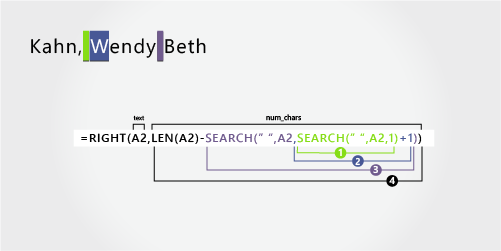
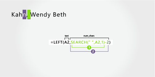
In this example, the last name comes before the first, and the middle name appears at the end. The comma marks the end of the last name, and a space separates each name component.
Copy the cells in the table and paste into an Excel worksheet at cell A1. The formula you see on the left will be displayed for reference, while Excel will automatically convert the formula on the right into the appropriate result.
Hint Before you paste the data into the worksheet, set the column widths of columns A and B to 250.
|
Example name |
Description |
|
Kahn, Wendy Beth |
Last name first, with comma |
|
Formula |
Result (first name) |
|
‘=MID(A2,SEARCH(» «,A2,1)+1,SEARCH(» «,A2,SEARCH(» «,A2,1)+1)-SEARCH(» «,A2,1)) |
=MID(A2,SEARCH(» «,A2,1)+1,SEARCH(» «,A2,SEARCH(» «,A2,1)+1)-SEARCH(» «,A2,1)) |
|
Formula |
Result (middle name) |
|
‘=RIGHT(A2,LEN(A2)-SEARCH(» «,A2,SEARCH(» «,A2,1)+1)) |
=RIGHT(A2,LEN(A2)-SEARCH(» «,A2,SEARCH(» «,A2,1)+1)) |
|
Formula |
Live Result (last name) |
|
‘=LEFT(A2, SEARCH(» «,A2,1)-2) |
=LEFT(A2, SEARCH(» «,A2,1)-2) |
-
First name
The first name starts with the seventh character from the left (W) and ends at the twelfth character (the second space). Because the first name occurs at the middle of the full name, you need to use the MID function to extract the first name.
The formula extracts six characters, starting from the seventh position.
Use the SEARCH function to find the value for start_num:
Search for the numeric position of the first space in A2, starting from the first character from the left. (6)
-
Add 1 to get the position of the character after the first space (W). This numeric position is the starting position of the first name. (6 + 1 = 7)
Use nested SEARCH functions to find the value for num_chars:
Search for the numeric position of the first space in A2, starting from the first character from the left. (6)
-
Add 1 to get the position of the character after the first space (W). The result is the character number at which you want to start searching for the second space. (6 + 1 = 7)
Search for the second space in A2, starting from the seventh position (W) found in step 4. (12)
-
Search for the numeric position of the first space in A2, starting from the first character from the left. (6)
-
Take the character number of the second space found in step 5 and subtract the character number of the first space found in step 6. The result is the number of characters MID extracts from the text string starting at the seventh position found in step 2. (12 — 6 = 6)
-
Middle name
The middle name starts four characters from the right (B), and ends at the first character from the right (h). This formula involves nesting SEARCH to find the first and second instances of space in the sixth and twelfth positions from the left.
The formula extracts four characters, starting from the right.
Use nested SEARCH and the LEN functions to find the value for start_num:
Search for the numeric position of the first space in A2, starting from the first character from the left. (6)
-
Add 1 to get the position of the character after the first space (W). The result is the character number at which you want to start searching for the second space. (6 + 1 = 7)
-
Search for the second instance of space in A2 starting from the seventh position (W) found in step 2. (12)
-
Count the total length of the text string in A2, and then subtract the number of characters from the left up to the second space found in step 3. The result is the number of characters to be extracted from the right of the full name. (16 — 12 = 4)
-
Last name
The last name starts with the first character from the left (K) and ends at the fourth character (n). The formula extracts four characters, starting from the left.
Use the SEARCH function to find the value for num_chars:
Search for the numeric position of the first space in A2, starting from the first character from the left. (6)
-
Subtract 2 to get the numeric position of the ending character of the last name (n). The result is the number of characters you want LEFT to extract. (6 — 2 =4)

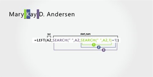
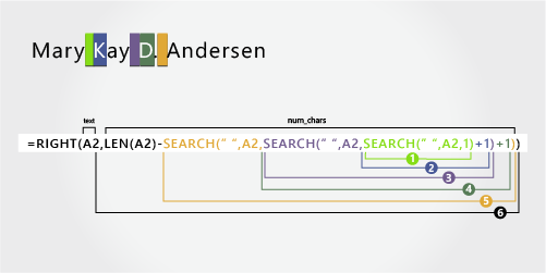
This example uses a two-part first name, Mary Kay. The second and third spaces separate each name component.
Copy the cells in the table and paste into an Excel worksheet at cell A1. The formula you see on the left will be displayed for reference, while Excel will automatically convert the formula on the right into the appropriate result.
Hint Before you paste the data into the worksheet, set the column widths of columns A and B to 250.
|
Example name |
Description |
|
Mary Kay D. Andersen |
Two-part first name |
|
Formula |
Result (first name) |
|
LEFT(A2, SEARCH(» «,A2,SEARCH(» «,A2,1)+1)) |
=LEFT(A2, SEARCH(» «,A2,SEARCH(» «,A2,1)+1)) |
|
Formula |
Result (middle initial) |
|
‘=MID(A2,SEARCH(» «,A2,SEARCH(» «,A2,1)+1)+1,SEARCH(» «,A2,SEARCH(» «,A2,SEARCH(» «,A2,1)+1)+1)-(SEARCH(» «,A2,SEARCH(» «,A2,1)+1)+1)) |
=MID(A2,SEARCH(» «,A2,SEARCH(» «,A2,1)+1)+1,SEARCH(» «,A2,SEARCH(» «,A2,SEARCH(» «,A2,1)+1)+1)-(SEARCH(» «,A2,SEARCH(» «,A2,1)+1)+1)) |
|
Formula |
Live Result (last name) |
|
‘=RIGHT(A2,LEN(A2)-SEARCH(» «,A2,SEARCH(» «,A2,SEARCH(» «,A2,1)+1)+1)) |
=RIGHT(A2,LEN(A2)-SEARCH(» «,A2,SEARCH(» «,A2,SEARCH(» «,A2,1)+1)+1)) |
-
First name
The first name starts with the first character from the left and ends at the ninth character (the second space). This formula involves nesting SEARCH to find the second instance of space from the left.
The formula extracts nine characters, starting from the left.
Use nested SEARCH functions to find the value for num_chars:
Search for the numeric position of the first space in A2, starting from the first character from the left. (5)
-
Add 1 to get the position of the character after the first space (K). The result is the character number at which you want to start searching for the second instance of space. (5 + 1 = 6)
-
Search for the second instance of space in A2, starting from the sixth position (K) found in step 2. The result is the number of characters LEFT extracts from the text string. (9)
-
Middle name
The middle name starts at the tenth position (D), and ends at the twelfth position (the third space). This formula involves nesting SEARCH to find the first, second, and third instances of space.
The formula extracts two characters from the middle, starting from the tenth position.
Use nested SEARCH functions to find the value for start_num:
Search for the numeric position of the first space in A2, starting from the first character from the left. (5)
-
Add 1 to get the character after the first space (K). The result is the character number at which you want to start searching for the second space. (5 + 1 = 6)
-
Search for the position of the second instance of space in A2, starting from the sixth position (K) found in step 2. The result is the number of characters LEFT extracts from the left. (9)
-
Add 1 to get the character after the second space (D). The result is the starting position of the middle name. (9 + 1 = 10)
Use nested SEARCH functions to find the value for num_chars:
Search for the numeric position of the character after the second space (D). The result is the character number at which you want to start searching for the third space. (10)
-
Search for the numeric position of the third space in A2, starting from the left. The result is the ending position of the middle name. (12)
-
Search for the numeric position of the character after the second space (D). The result is the beginning position of the middle name. (10)
-
Take the character number of the third space, found in step 6, and subtract the character number of “D”, found in step 7. The result is the number of characters MID extracts from the text string starting at the tenth position found in step 4. (12 — 10 = 2)
-
Last name
The last name starts eight characters from the right. This formula involves nesting SEARCH to find the first, second, and third instances of space in the fifth, ninth, and twelfth positions.
The formula extracts eight characters from the right.
Use nested SEARCH and the LEN functions to find the value for num_chars:
Search for the numeric position of the first space in A2, starting from the left. (5)
-
Add 1 to get the character after the first space (K). The result is the character number at which you want to start searching for the space. (5 + 1 = 6)
-
Search for the second space in A2, starting from the sixth position (K) found in step 2. (9)
-
Add 1 to get the position of the character after the second space (D). The result is the starting position of the middle name. (9 + 1 = 10)
-
Search for the numeric position of the third space in A2, starting from the left. The result is the ending position of the middle name. (12)
-
Count the total length of the text string in A2, and then subtract the number of characters from the left up to the third space found in step 5. The result is the number of characters to be extracted from the right of the full name. (20 — 12 =


This example uses a three-part last name: Barreto de Mattos. The first space marks the end of the first name and the beginning of the last name.
Copy the cells in the table and paste into an Excel worksheet at cell A1. The formula you see on the left will be displayed for reference, while Excel will automatically convert the formula on the right into the appropriate result.
Hint Before you paste the data into the worksheet, set the column widths of columns A and B to 250.
|
Example name |
Description |
|
Paula Barreto de Mattos |
Three-part last name |
|
Formula |
Result (first name) |
|
‘=LEFT(A2, SEARCH(» «,A2,1)) |
=LEFT(A2, SEARCH(» «,A2,1)) |
|
Formula |
Result (last name) |
|
RIGHT(A2,LEN(A2)-SEARCH(» «,A2,1)) |
=RIGHT(A2,LEN(A2)-SEARCH(» «,A2,1)) |
-
First name
The first name starts with the first character from the left (P) and ends at the sixth character (the first space). The formula extracts six characters from the left.
Use the Search function to find the value for num_chars:
Search for the numeric position of the first space in A2, starting from the left. (6)
-
Last name
The last name starts seventeen characters from the right (B) and ends with first character from the right (s). The formula extracts seventeen characters from the right.
Use the LEN and SEARCH functions to find the value for num_chars:
Search for the numeric position of the first space in A2, starting from the left. (6)
-
Count the total length of the text string in A2, and then subtract the number of characters from the left up to the first space, found in step 1. The result is the number of characters to be extracted from the right of the full name. (23 — 6 = 17)


This example uses a two-part last name: van Eaton. The first space marks the end of the first name and the beginning of the last name.
Copy the cells in the table and paste into an Excel worksheet at cell A1. The formula you see on the left will be displayed for reference, while Excel will automatically convert the formula on the right into the appropriate result.
Hint Before you paste the data into the worksheet, set the column widths of columns A and B to 250.
|
Example name |
Description |
|
James van Eaton |
Two-part last name |
|
Formula |
Result (first name) |
|
‘=LEFT(A2, SEARCH(» «,A2,1)) |
=LEFT(A2, SEARCH(» «,A2,1)) |
|
Formula |
Result (last name) |
|
‘=RIGHT(A2,LEN(A2)-SEARCH(» «,A2,1)) |
=RIGHT(A2,LEN(A2)-SEARCH(» «,A2,1)) |
-
First name
The first name starts with the first character from the left (J) and ends at the eighth character (the first space). The formula extracts six characters from the left.
Use the SEARCH function to find the value for num_chars:
Search for the numeric position of the first space in A2, starting from the left. (6)
-
Last name
The last name starts with the ninth character from the right (v) and ends at the first character from the right (n). The formula extracts nine characters from the right of the full name.
Use the LEN and SEARCH functions to find the value for num_chars:
Search for the numeric position of the first space in A2, starting from the left. (6)
-
Count the total length of the text string in A2, and then subtract the number of characters from the left up to the first space, found in step 1. The result is the number of characters to be extracted from the right of the full name. (15 — 6 = 9)


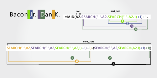
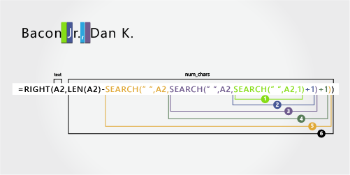
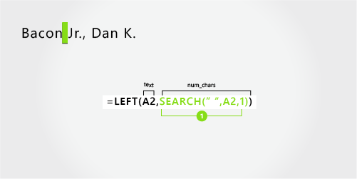
In this example, the last name comes first, followed by the suffix. The comma separates the last name and suffix from the first name and middle initial.
Copy the cells in the table and paste into an Excel worksheet at cell A1. The formula you see on the left will be displayed for reference, while Excel will automatically convert the formula on the right into the appropriate result.
Hint Before you paste the data into the worksheet, set the column widths of columns A and B to 250.
|
Example name |
Description |
|
Bacon Jr., Dan K. |
Last name and suffix first, with comma |
|
Formula |
Result (first name) |
|
‘=MID(A2,SEARCH(» «,A2,SEARCH(» «,A2,1)+1)+1,SEARCH(» «,A2,SEARCH(» «,A2,SEARCH(» «,A2,1)+1)+1)-SEARCH(» «,A2,SEARCH(» «,A2,1)+1)) |
=MID(A2,SEARCH(» «,A2,SEARCH(» «,A2,1)+1)+1,SEARCH(» «,A2,SEARCH(» «,A2,SEARCH(» «,A2,1)+1)+1)-SEARCH(» «,A2,SEARCH(» «,A2,1)+1)) |
|
Formula |
Result (middle initial) |
|
‘=RIGHT(A2,LEN(A2)-SEARCH(» «,A2,SEARCH(» «,A2,SEARCH(» «,A2,1)+1)+1)) |
=RIGHT(A2,LEN(A2)-SEARCH(» «,A2,SEARCH(» «,A2,SEARCH(» «,A2,1)+1)+1)) |
|
Formula |
Result (last name) |
|
‘=LEFT(A2, SEARCH(» «,A2,1)) |
=LEFT(A2, SEARCH(» «,A2,1)) |
|
Formula |
Result (suffix) |
|
‘=MID(A2,SEARCH(» «, A2,1)+1,(SEARCH(» «,A2,SEARCH(» «,A2,1)+1)-2)-SEARCH(» «,A2,1)) |
=MID(A2,SEARCH(» «, A2,1)+1,(SEARCH(» «,A2,SEARCH(» «,A2,1)+1)-2)-SEARCH(» «,A2,1)) |
-
First name
The first name starts with the twelfth character (D) and ends with the fifteenth character (the third space). The formula extracts three characters, starting from the twelfth position.
Use nested SEARCH functions to find the value for start_num:
Search for the numeric position of the first space in A2, starting from the left. (6)
-
Add 1 to get the character after the first space (J). The result is the character number at which you want to start searching for the second space. (6 + 1 = 7)
-
Search for the second space in A2, starting from the seventh position (J), found in step 2. (11)
-
Add 1 to get the character after the second space (D). The result is the starting position of the first name. (11 + 1 = 12)
Use nested SEARCH functions to find the value for num_chars:
Search for the numeric position of the character after the second space (D). The result is the character number at which you want to start searching for the third space. (12)
-
Search for the numeric position of the third space in A2, starting from the left. The result is the ending position of the first name. (15)
-
Search for the numeric position of the character after the second space (D). The result is the beginning position of the first name. (12)
-
Take the character number of the third space, found in step 6, and subtract the character number of “D”, found in step 7. The result is the number of characters MID extracts from the text string starting at the twelfth position, found in step 4. (15 — 12 = 3)
-
Middle name
The middle name starts with the second character from the right (K). The formula extracts two characters from the right.
Search for the numeric position of the first space in A2, starting from the left. (6)
-
Add 1 to get the character after the first space (J). The result is the character number at which you want to start searching for the second space. (6 + 1 = 7)
-
Search for the second space in A2, starting from the seventh position (J), found in step 2. (11)
-
Add 1 to get the character after the second space (D). The result is the starting position of the first name. (11 + 1 = 12)
-
Search for the numeric position of the third space in A2, starting from the left. The result is the ending position of the middle name. (15)
-
Count the total length of the text string in A2, and then subtract the number of characters from the left up to the third space, found in step 5. The result is the number of characters to be extracted from the right of the full name. (17 — 15 = 2)
-
Last name
The last name starts at the first character from the left (B) and ends at sixth character (the first space). Therefore, the formula extracts six characters from the left.
Use the SEARCH function to find the value for num_chars:
Search for the numeric position of the first space in A2, starting from the left. (6)
-
Suffix
The suffix starts at the seventh character from the left (J), and ends at ninth character from the left (.). The formula extracts three characters, starting from the seventh character.
Use the SEARCH function to find the value for start_num:
Search for the numeric position of the first space in A2, starting from the left. (6)
-
Add 1 to get the character after the first space (J). The result is the starting position of the suffix. (6 + 1 = 7)
Use nested SEARCH functions to find the value for num_chars:
Search for the numeric position of the first space in A2, starting from the left. (6)
-
Add 1 to get the numeric position of the character after the first space (J). The result is the character number at which you want to start searching for the second space. (7)
-
Search for the numeric position of the second space in A2, starting from the seventh character found in step 4. (11)
-
Subtract 1 from the character number of the second space found in step 4 to get the character number of “,”. The result is the ending position of the suffix. (11 — 1 = 10)
-
Search for the numeric position of the first space. (6)
-
After finding the first space, add 1 to find the next character (J), also found in steps 3 and 4. (7)
-
Take the character number of “,” found in step 6, and subtract the character number of “J”, found in steps 3 and 4. The result is the number of characters MID extracts from the text string starting at the seventh position, found in step 2. (10 — 7 = 3)

In this example, the first name is at the beginning of the string and the suffix is at the end, so you can use formulas similar to Example 2: Use the LEFT function to extract the first name, the MID function to extract the last name, and the RIGHT function to extract the suffix.
Copy the cells in the table and paste into an Excel worksheet at cell A1. The formula you see on the left will be displayed for reference, while Excel will automatically convert the formula on the right into the appropriate result.
Hint Before you paste the data into the worksheet, set the column widths of columns A and B to 250.
|
Example name |
Description |
|
Gary Altman III |
First and last name with suffix |
|
Formula |
Result (first name) |
|
‘=LEFT(A2, SEARCH(» «,A2,1)) |
=LEFT(A2, SEARCH(» «,A2,1)) |
|
Formula |
Result (last name) |
|
‘=MID(A2,SEARCH(» «,A2,1)+1,SEARCH(» «,A2,SEARCH(» «,A2,1)+1)-(SEARCH(» «,A2,1)+1)) |
=MID(A2,SEARCH(» «,A2,1)+1,SEARCH(» «,A2,SEARCH(» «,A2,1)+1)-(SEARCH(» «,A2,1)+1)) |
|
Formula |
Result (suffix) |
|
‘=RIGHT(A2,LEN(A2)-SEARCH(» «,A2,SEARCH(» «,A2,1)+1)) |
=RIGHT(A2,LEN(A2)-SEARCH(» «,A2,SEARCH(» «,A2,1)+1)) |
-
First name
The first name starts at the first character from the left (G) and ends at the fifth character (the first space). Therefore, the formula extracts five characters from the left of the full name.
Search for the numeric position of the first space in A2, starting from the left. (5)
-
Last name
The last name starts at the sixth character from the left (A) and ends at the eleventh character (the second space). This formula involves nesting SEARCH to find the positions of the spaces.
The formula extracts six characters from the middle, starting from the sixth character.
Use the SEARCH function to find the value for start_num:
Search for the numeric position of the first space in A2, starting from the left. (5)
-
Add 1 to get the position of the character after the first space (A). The result is the starting position of the last name. (5 + 1 = 6)
Use nested SEARCH functions to find the value for num_chars:
Search for the numeric position of the first space in A2, starting from the left. (5)
-
Add 1 to get the position of the character after the first space (A). The result is the character number at which you want to start searching for the second space. (5 + 1 = 6)
-
Search for the numeric position of the second space in A2, starting from the sixth character found in step 4. This character number is the ending position of the last name. (12)
-
Search for the numeric position of the first space. (5)
-
Add 1 to find the numeric position of the character after the first space (A), also found in steps 3 and 4. (6)
-
Take the character number of the second space, found in step 5, and then subtract the character number of “A”, found in steps 6 and 7. The result is the number of characters MID extracts from the text string, starting at the sixth position, found in step 2. (12 — 6 = 6)
-
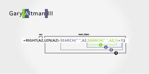
Suffix
The suffix starts three characters from the right. This formula involves nesting SEARCH to find the positions of the spaces.
Use nested SEARCH and the LEN functions to find the value for num_chars:
Search for the numeric position of the first space in A2, starting from the left. (5)
-
Add 1 to get the character after the first space (A). The result is the character number at which you want to start searching for the second space. (5 + 1 = 6)
-
Search for the second space in A2, starting from the sixth position (A), found in step 2. (12)
-
Count the total length of the text string in A2, and then subtract the number of characters from the left up to the second space, found in step 3. The result is the number of characters to be extracted from the right of the full name. (15 — 12 = 3)

In this example, the full name is preceded by a prefix, and you use formulas similar to Example 2: the MID function to extract the first name, the RIGHT function to extract the last name.
Copy the cells in the table and paste into an Excel worksheet at cell A1. The formula you see on the left will be displayed for reference, while Excel will automatically convert the formula on the right into the appropriate result.
Hint Before you paste the data into the worksheet, set the column widths of columns A and B to 250.
|
Example name |
Description |
|
Mr. Ryan Ihrig |
With prefix |
|
Formula |
Result (first name) |
|
‘=MID(A2,SEARCH(» «,A2,1)+1,SEARCH(» «,A2,SEARCH(» «,A2,1)+1)-(SEARCH(» «,A2,1)+1)) |
=MID(A2,SEARCH(» «,A2,1)+1,SEARCH(» «,A2,SEARCH(» «,A2,1)+1)-(SEARCH(» «,A2,1)+1)) |
|
Formula |
Result (last name) |
|
‘=RIGHT(A2,LEN(A2)-SEARCH(» «,A2,SEARCH(» «,A2,1)+1)) |
=RIGHT(A2,LEN(A2)-SEARCH(» «,A2,SEARCH(» «,A2,1)+1)) |
-
First name
The first name starts at the fifth character from the left (R) and ends at the ninth character (the second space). The formula nests SEARCH to find the positions of the spaces. It extracts four characters, starting from the fifth position.
Use the SEARCH function to find the value for the start_num:
Search for the numeric position of the first space in A2, starting from the left. (4)
-
Add 1 to get the position of the character after the first space (R). The result is the starting position of the first name. (4 + 1 = 5)
Use nested SEARCH function to find the value for num_chars:
Search for the numeric position of the first space in A2, starting from the left. (4)
-
Add 1 to get the position of the character after the first space (R). The result is the character number at which you want to start searching for the second space. (4 + 1 = 5)
-
Search for the numeric position of the second space in A2, starting from the fifth character, found in steps 3 and 4. This character number is the ending position of the first name. (9)
-
Search for the first space. (4)
-
Add 1 to find the numeric position of the character after the first space (R), also found in steps 3 and 4. (5)
-
Take the character number of the second space, found in step 5, and then subtract the character number of “R”, found in steps 6 and 7. The result is the number of characters MID extracts from the text string, starting at the fifth position found in step 2. (9 — 5 = 4)
-
Last name
The last name starts five characters from the right. This formula involves nesting SEARCH to find the positions of the spaces.
Use nested SEARCH and the LEN functions to find the value for num_chars:
Search for the numeric position of the first space in A2, starting from the left. (4)
-
Add 1 to get the position of the character after the first space (R). The result is the character number at which you want to start searching for the second space. (4 + 1 = 5)
-
Search for the second space in A2, starting from the fifth position (R), found in step 2. (9)
-
Count the total length of the text string in A2, and then subtract the number of characters from the left up to the second space, found in step 3. The result is the number of characters to be extracted from the right of the full name. (14 — 9 = 5)


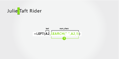
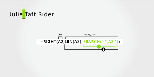
This example uses a hyphenated last name. A space separates each name component.
Copy the cells in the table and paste into an Excel worksheet at cell A1. The formula you see on the left will be displayed for reference, while Excel will automatically convert the formula on the right into the appropriate result.
Hint Before you paste the data into the worksheet, set the column widths of columns A and B to 250.
|
Example name |
Description |
|
Julie Taft-Rider |
Hyphenated last name |
|
Formula |
Result (first name) |
|
‘=LEFT(A2, SEARCH(» «,A2,1)) |
=LEFT(A2, SEARCH(» «,A2,1)) |
|
Formula |
Result (last name) |
|
‘=RIGHT(A2,LEN(A2)-SEARCH(» «,A2,1)) |
=RIGHT(A2,LEN(A2)-SEARCH(» «,A2,1)) |
-
First name
The first name starts at the first character from the left and ends at the sixth position (the first space). The formula extracts six characters from the left.
Use the SEARCH function to find the value of num_chars:
Search for the numeric position of the first space in A2, starting from the left. (6)
-
Last name
The entire last name starts ten characters from the right (T) and ends at the first character from the right (r).
Use the LEN and SEARCH functions to find the value for num_chars:
Search for the numeric position of the space in A2, starting from the first character from the left. (6)
-
Count the total length of the text string to be extracted, and then subtract the number of characters from the left up to the first space, found in step 1. (16 — 6 = 10)
Need more help?
When data is imported into Excel it can be in many formats depending on the source application that has provided it.
For example, it could contain names and addresses of customers or employees, but this all ends up as a continuous text string in one column of the worksheet, instead of being separated out into individual columns e.g. name, street, city.
You can split the data by using a common delimiter character. A delimiter character is usually a comma, tab, space, or semi-colon. This character separates each chunk of data within the text string.
A big advantage of using a delimiter character is that it does not rely on fixed widths within the text. The delimiter indicates exactly where to split the text.
You may need to split the data because you may want to sort the data using a certain part of the address or to be able to filter on a particular component. If the data is used in a pivot table, you may need to have the name and address as different fields within it.
This article shows you eight ways to split the text into the component parts required by using a delimiter character to indicate the split points.
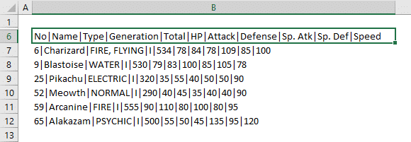
Sample Data
The above sample data will be used in all the following examples. Download the example file to get the sample data plus the various solutions for extracting data based on delimiters.
Excel Functions to Split Text
There are several Excel functions that can be used to split and manipulate text within a cell.
LEFT Function
The LEFT function returns the number of characters from the left of the text.
Syntax
= LEFT ( Text, [Number] )- Text – This is the text string that you wish to extract from. It can also be a valid cell reference within a workbook.
- Number [Optional] – This is the number of characters that you wish to extract from the text string. The value must be greater than or equal to zero. If the value is greater than the length of the text string, then all characters will be returned. If the value is omitted, then the value is assumed to be one.
RIGHT Function
The RIGHT function returns the number of characters from the right of the text.
Syntax
= RIGHT ( Text, [Number] )The parameters work in the same way as for the LEFT function described above.
FIND Function
The FIND function returns the position of specified text within a text string. This can be used for locating a delimiter character. Note that the search is case-sensitive.
Syntax
= FIND (SubText, Text, [Start])- SubText – This is a text string that you want to search for.
- Text – This is the text string which is to be searched.
- Start [Optional] – The starting position for the search.
LEN Function
The LEN function will give the length by number of characters of a text string.
Syntax
= LEN ( Text )- Text – This is the text string of which you want to determine the character count.
Extracting Data with the LEFT, RIGHT, FIND and LEN Functions
Using the first row (B3) of the sample data, these functions can be combined to split a text string into sections using a delimiter character.
= FIND ( ",", B3 )You use the FIND function to get the position of the first delimiter character. This will return the value 18.
= LEFT ( B3, FIND( ",", B3 ) - 1 )You can then use the LEFT function to extract the first component of the text string.
Note that FIND gets the position of the first delimiter, but you need to subtract 1 from it so as to not include the delimiter character.
This will return Tabbie O’Hallagan.
= RIGHT ( B3, LEN ( B3 ) - FIND ( ",", B3 ) )It is more complicated to get the next components of the text string. You need to remove the first component from the text by using the above formula.
This formula takes the length of the original text, finds the first delimiter position, which then calculates how many characters are left in the text string after that delimiter.
The RIGHT function then truncates off all the characters up to and including that first delimiter so that the text string gets shorter and shorter as each delimiter character is found.
This will return 056 Dennis Park, Greda, Croatia, 44273
You can now use FIND to locate the next delimiter and the LEFT function to extract the next component, using the same methodology as above.
Repeat for all delimiters, and this will split the text string into component parts.
FILTERXML Function as a Dynamic Array
If you’re using Excel for Microsoft 365, then you can use the FILTERXML function to split text with output as a dynamic array.
You can split a text string by turning it into an XML string by changing the delimiter characters to XML tags. This way you can use the FILTERXML function to extract data.
XML tags are user defined, but in this example, s will represent a sub-node and t will represent the main node.
= "<t><s>" & SUBSTITUTE ( B2, ",", "</s><s>" ) & "</s></t>"Use the above formula to insert the XML tags into your text string.
<t><s>Name</s><s>Street</s><s>City</s><s>Country</s><s>Post Code</s></t>This will return the above formula in the example.
Note that each of the nodes defined is followed by a closing node with a backslash. These XML tags define the start and finish of each section of the text, and effectively act in the same way as delimiters.
=TRANSPOSE(
    FILTERXML(
        "<t><s>" &
        SUBSTITUTE(
            B3,
            ",",
            "</s><s>"
        ) & "</s></t>",
        "//s"
    )
)
The above formula will insert the XML tags into the original string and then use these to split out the items into an array.
As seen above, the array will spill each item into a separate cell. Using the TRANSPOSE function causes the array to spill horizontally instead of vertically.
FILTERXML Function to Split Text
If your version of Excel doesn’t have dynamic arrays, then you can still use the FILTERXML function to extract individual items.
= FILTERXML (
    "<t><s>" &
    SUBSTITUTE (
        B3,
        ",",
        "</s><s>"
    ) & "</s></t>",
    "//s"
)
You can now break the string into sections using the above FILTERXML formula.
This will return the first section Tabbie O’Hallagan.
= FILTERXML (
    "<t><s>" &
    SUBSTITUTE (
        B3,
        ",",
        "</s><s>"
    ) & "</s></t>",
    "//s[2]"
)
To return the next section, use the above formula.
This will return the second section of the text string 056 Dennis Park.
You can use this same pattern to return any part of the sample text, just change the [2] found in the formula accordingly.
Flash Fill to Split Text
Flash Fill allows you to put in an example of how you want your data split.
You can check out this guide on using flash fill to clean your data for more details.
You then select the first cell of where you want your data to split and click on Flash Fill. Excel will populate the remaining rows from your example.
Using the sample data, enter Name into cell C2, then Tabbie O’Hallagan into cell C3.
Flash fill should automatically fill in the remaining data names from the sample data. If it doesn’t, you can select cell C4, and click on the Flash Fill icon in the Data Tools group of the Data tab of the Excel ribbon.
Similarly, you can add Street into cell D2, City into cell E2, Country into cell F2, and Post Code into cell G2.
Select the subsequent cells (D2 to G2) individually, and click on the Flash Fill icon. The rest of the text components will be populated into these columns.
Text to Columns Command to Split Text
This Excel functionality can be used to split text in a cell into sections based on a delimiter character.
- Select the entire sample data range (B2:B12).
- Click on the Data tab in the Excel ribbon.
- Click on the Text to Columns icon in the Data Tools group of the Excel ribbon and a wizard will appear to help you set up how the text will be split.
- Select Delimited on the option buttons.
- Press the Next button.
- Select Comma as the delimiter, and uncheck any other delimiters.
- Press the Next button.
- The Data Preview window will display how your data will be split. Choose a location to place the output.
- Click on Finish button.
Your data will now be displayed in columns on your worksheet.
Convert the Data into a CSV File
This will only work with commas as delimiters, since a CSV (comma separated value) file depends on commas to separate the values.
Open Notepad and copy and paste the sample data into it. You can open Notepad by typing Notepad into the search box at the left of the Windows task bar or locate it in the application list.
Once you have copied the data into Notepad, save it off by using File ➜ Save As from the menu. Enter a filename with a .csv suffix e.g. Split Data.csv.
You can then open this file in Excel. Select the csv file in the browser file type drop down and click OK. Your data will automatically appear with each component in separate columns.
VBA to Split Text
VBA is the programming language that sits behind Excel and allows you to write your own code to manipulate data, or to even create your own functions.
To access the Visual Basic Editor (VBE), you use Alt + F11.
Sub SplitText()

Dim MyArray() As String, Count As Long, i As Variant

For n = 2 To 12
	MyArray = Split(Cells(n, 2), ",")
	Count = 3
	For Each i In MyArray
		Cells(n, Count) = i
		Count = Count + 1
	Next i
Next n

End Sub
Click on Insert in the menu bar, and click on Module. A new pane will appear for the module. Paste in the above code.
This code creates a single dimensional array called MyArray. It then iterates through the sample data (rows 2 to 12) and uses the VBA Split function to populate MyArray.
The split function uses a comma delimiter, so that each section of the text becomes an element of the array.
A counter variable is set to 3 which represents column C, which will be the first column for the split data to be displayed.
The code then iterates through each element in the array and populates each cell with the element. Cell references are based on n for the row, and Count for the column.
The variable Count is incremented in each loop so that the data fills across the row, and then downwards.
Power Query to Split Text
Power Query in Excel allows a column to be manipulated into sections using a delimiter character.
Related posts:
- Introduction to power query
- Power query tips and tricks
- Introduction to power query M code
The first thing to do is to define your data source, which is the sample data that you entered into you Excel worksheet.
Click on the Data tab in the Excel ribbon, and then click on Get Data in the Get & Transform Data group of the ribbon.
Click on From File in the first drop down, and then click on From Workbook in the second drop down.
This will display a file browser. Locate your sample data file (the file that you have open) and click on OK.
A navigation pop-up will be displayed showing all the worksheets within your workbook. Click on the worksheet which has the sample data and this will show a preview of the data.
Expand the tree of data in the left-hand pane to show the preview of the existing data.
Click on Transform Data and this will display the Power Query Editor.
Make sure that the single column with the data in it is highlighted. Click on the Split Column icon in the Transform group of the ribbon. Click on By Delimiter in the drop down that appears.
This will display a pop-up window which allows you to select your delimiter. The default is a comma.
Click OK and the data will be transformed into separate columns.
Click on Close and Load in the Close group of the ribbon, and a new worksheet will be added to your workbook with a table of the data in the new format.
Power Pivot Calculated Column to Split Text
You can use Power Pivot to split the text by using calculated columns.
Click on the Power Pivot tab in the Excel ribbon and then click on the Add to Data Model icon in the Tables group.
Your data will be automatically detected and a pop-up will show the location. If this is not the correct location, then it can be re-set here.
Leave the My table has headers check box un-ticked in the pop-up, as we want to split the header as well.
Click on OK and a preview screen will be displayed.
Right-click on the header for your data column (Column1) and click on Insert Column in the pop-up menu. This will insert a calculated column where a formula can be entered.
= LEFT ( [Column1], FIND ( ",", [Column1] ) - 1 )In the formula bar, insert the above formula.
This works in a similar way to the functions described in method 1 of this article.
This formula will provide the Name component within the text string.
Insert another calculated column using the same methodology as the first calculated column.
= LEFT (
    RIGHT ( [Column1], LEN ( [column1] ) - LEN ( [Calculated Column 1] ) - 1 ),
    FIND (
        ",",
        RIGHT ( [Column1], LEN ( [column1] ) - LEN ( [Calculated Column 1] ) - 1 )
    ) - 1
)
Insert the above formula into the formula bar.
This is a complicated formula, and you may wish to break it into sections using several calculated columns.
This will provide the Street component in the text string.
You can continue modifying the formula to create calculated columns for all the other components of the text string.
The problem with a pivot table is that it needs a numeric value as well as text values. As the sample data is text only, a numeric value needs to be added.
Click on the first cell in the Add Column column and enter the formula =1 in the formula bar.
This will add the value of 1 all the way down that column. Click on the Pivot Table icon in the Home tab of the ribbon.
Click on Pivot Table in the pop-up menu. Specify the location of your pivot table in the first pop-up window and click OK. If the Pivot Table Fields pane does not automatically display, right click on the pivot table skeleton and select Show Field List.
Click on the Calculated Columns in the Field List and place these in the Rows window.
our pivot table will now show the individual components of the text string.
Conclusions
Dealing with comma or other delimiter separated data can be a big pain if you don’t know how to extract each item into its own cell.
Thankfully, Excel has quite a few options that will help with this common task.
Which one do you prefer to use?
About the Author
John is a Microsoft MVP and qualified actuary with over 15 years of experience. He has worked in a variety of industries, including insurance, ad tech, and most recently Power Platform consulting. He is a keen problem solver and has a passion for using technology to make businesses more efficient.
In this guide, we’re going to show you how to split text in Excel by a delimiter.
Download Workbook
We have a sample data which contains concatenated values separated by “|” characters. It is important that the data includes a specific delimiter character between each chunk of data to make splitting text easier.
Text to Columns feature for splitting text
When splitting text in Excel, the Text to Columns is one of the most common methods. You can use the Text to Columns feature with all versions of Excel. This feature can split text by a specific character count or delimiter.
- Start with selecting your data. You can use more than one cell in a column.
- Click Data > Text to Columns in the Ribbon.
- On the first step of the wizard, you have 2 options to choose from — these are slicing methods. Since our data in this example is split by delimiters, our choice is going to be Delimited.
- Click Next to continue
- Select the delimiters suitable to your data or choose a character length and click Next.
- Choose corresponding data types for the columns and the destination cell. Please note that if the destination cell is the same cell as where your data is, the original data will be overwritten.
- Click Finish to see the outcome.
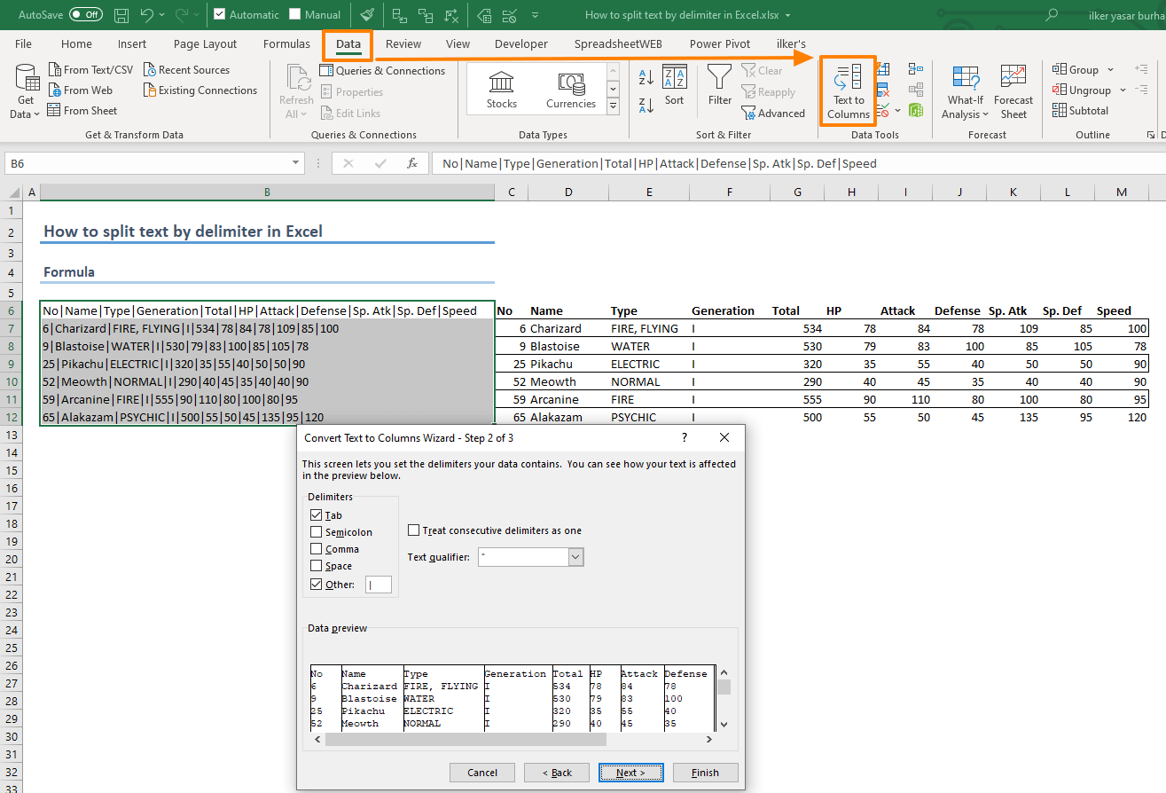
Using formulas to split text
Excel has a variety of text formulas that you can use to locate delimiters and parse data. When using formulas to do so, Excel automatically updates the parsed values when the source is updated.
The formula used in this example uses Microsoft 365’s dynamic array feature, which allows you to populate multiple cells without using array formulas. If you can see the SEQUENCE formula, you can use this method.
Syntax
=TRIM(MID(SUBSTITUTE( text, separator, REPT( “ “, LEN( text ))),(SEQUENCE( 1, column count ) — 1 ) * LEN( text ) + 1,LEN( text )))
How it works
The formula replaces each separator character with space characters first. (see SUBSTITUTE) The number of space characters will be equal to the original string’s character count, which is enough number of spaces to separate each string block (see REPT and LEN).
The SEQUENCE function generates an array of numbers starting with 1, up to the number of maximum columns. Multiplying these sequential numbers with the length of the original string returns character numbers indicating the start of each block.
This approach uses the MID function to parse each string block with given start character number and the number of characters to return. Since the separators are replaced with space characters, each parsed block includes these spaces around the actual string. The TRIM function then removes these spaces.

Flash Fill
The Flash Fill is an Excel tool which can detect the pattern when entering data. A common example is to separate or merge first name and last names. Let’s say column A contains the first name — last name combinations. If you type in the corresponding first name in the same row for column B, Excel shows you a preview for the rest of the column.
Please note that the Flash Fill is available for Excel 2013 and newer versions only.
You can see the same behavior with strings using delimiters to separate data. Just select a cell in the adjacent column and start typing. Occasionally Excel will display a preview. If not, press Ctrl + E like below to split your text.

Power Query
Power Query is a powerful feature, not only for splitting text, but for data management in general. Power Query comes with its own text splitting tool which allows you to split text in multiple ways, like by delimiters, number of characters, or case of letters.
If you are using Excel 2016 or newer — including Microsoft 365 — you can find Power Query options under the Data tab’s Get & Transform section. Excel 2010 and 2013 users should download and install the Power Query as an add-in.
- Select the cells containing the text.
- Click Data > From Sheet. If the data is not in an Excel Table, Excel converts it into an Excel Table first.
- Once the Power Query window is open, find the Split Column under the Transform tab and click to see the options.
- Select the approach that fits your data layout. The data in our example is using By Delimiter since the data is separated by “|”.
- Power Query will show the delimiter character. If you are not seeing the expected delimiter, choose from the list or enter it yourself.
- Click OK to split text.
- If your data includes headers in its first row, like our example does, click Transform > Use First Row as Headers to keep them as headers.
- One you satisfied with the result, click the Home > Close & Load button to move the split data into your workbook.

VBA
VBA is the last text splitting option we want to show in this article. You can use VBA in two ways to split text:
- By calling the Text to Columns feature using VBA,
- Using VBA’s Split function to create array of sub-strings and using a loop to distribute the sub-strings into adjacent cells in the same row.
Text to Columns by VBA
The following code can split data from selected cells into the adjacent columns. Note that each supported delimiter is listed as an argument which you can enable or disable by giving them either True or False. Briefly, True means that you want to set that argument as a delimiter and False means ignore that character.

An easy way to generate a VBA code to split text is to record a macro. Start a recording section using the Record Macro button in the Developer tab, and use the Text to Columns feature. Once the recording is stopped, Excel will save the code for what you did during recording.
The code:
Sub VBATextToColumns_Multiple()
Dim MyRange As Range
Set MyRange = Selection ‘To work on a static range replace Selection via Range object, e.g., Range(“B6:B12”)
MyRange.TextToColumns _
Destination:=MyRange(1, 1).Offset(, 1), _
DataType:=xlDelimited, _
TextQualifier:=xlDoubleQuote, _
ConsecutiveDelimiter:=False, _
Tab:=True, _
SemiColon:=False, _
Comma:=False, _
Space:=False, _
Other:=True, _
OtherChar:=»|»
End Sub
Split Function
Split function can be useful if you want to keep the split blocks in an array. You can only use this method for splitting because of the single delimiter constraint. The following code loops through each cell in a selected column, splits and stores text by the delimiter “|”, and uses another loop to populate the values in the array on cells. The final EntireColumn.AutoFit command adjusts the column widths.

The code:
Sub SplitText()
Dim StringArray() As String, Cell As Range, i As Integer
For Each Cell In Selection ‘To work on a static range replace Selection via Range object, e.g., Range(“B6:B12”)
StringArray = Split(Cell, «|») ‘Change the delimiter with a character suits your data
For i = 0 To UBound(StringArray)
Cell.Offset(, i + 1) = StringArray(i)
Cell.Offset(, i + 1).EntireColumn.AutoFit ‘This is for column width and optional.
Next i
Next
End Sub