
If you find yourself needing to expand or reduce Excel’s row widths and column heights, there are several ways to adjust them. The table below shows the minimum, maximum and default sizes for each based on a point scale.
|
Type |
Min |
Max |
Default |
|---|---|---|---|
|
Column |
0 (hidden) |
255 |
8.43 |
|
Row |
0 (hidden) |
409 |
15.00 |
Notes:
-
If you are working in Page Layout view (View tab, Workbook Views group, Page Layout button), you can specify a column width or row height in inches, centimeters and millimeters. The measurement unit is in inches by default. Go to File > Options > Advanced > Display > select an option from the Ruler Units list. If you switch to Normal view, then column widths and row heights will be displayed in points.
-
Individual rows and columns can only have one setting. For example, a single column can have a 25 point width, but it can’t be 25 points wide for one row, and 10 points for another.

Set a column to a specific width
-
Select the column or columns that you want to change.
-
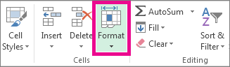
On the Home tab, in the Cells group, click Format.

-
Under Cell Size, click Column Width.
-
In the Column width box, type the value that you want.
-
Click OK.
Tip: To quickly set the width of a single column, right-click the selected column, click Column Width, type the value that you want, and then click OK.
-
Select the column or columns that you want to change.
-
On the Home tab, in the Cells group, click Format.
-
Under Cell Size, click AutoFit Column Width.
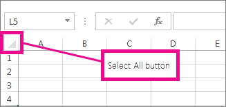
Note: To quickly autofit all columns on the worksheet, click the Select All button, and then double-click any boundary between two column headings.
-
Select a cell in the column that has the width that you want to use.
-
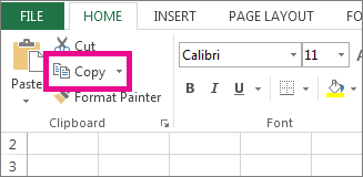
Press Ctrl+C, or on the Home tab, in the Clipboard group, click Copy.
-
Right-click a cell in the target column, point to Paste Special, and then click the Keep Source Columns Widths
button.
 button.
The value for the default column width indicates the average number of characters of the standard font that fit in a cell. You can specify a different number for the default column width for a worksheet or workbook.
-
Do one of the following:
-
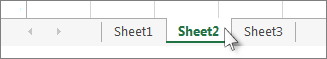
To change the default column width for a worksheet, click its sheet tab.
-
To change the default column width for the entire workbook, right-click a sheet tab, and then click Select All Sheets on the shortcut menu.
-
-
On the Home tab, in the Cells group, click Format.
-
Under Cell Size, click Default Width.
-
In the Standard column width box, type a new measurement, and then click OK.
Do one of the following:
-
To change the width of one column, drag the boundary on the right side of the column heading until the column is the width that you want.
-
To change the width of multiple columns, select the columns that you want to change, and then drag a boundary to the right of a selected column heading.
-
To change the width of columns to fit the contents, select the column or columns that you want to change, and then double-click the boundary to the right of a selected column heading.
-
To change the width of all columns on the worksheet, click the Select All button, and then drag the boundary of any column heading.
-
Select the row or rows that you want to change.
-
On the Home tab, in the Cells group, click Format.
-
Under Cell Size, click Row Height.
-
In the Row height box, type the value that you want, and then click OK.
-
Select the row or rows that you want to change.
-
On the Home tab, in the Cells group, click Format.
-
Under Cell Size, click AutoFit Row Height.
Tip: To quickly autofit all rows on the worksheet, click the Select All button, and then double-click the boundary below one of the row headings.
Do one of the following:
-
To change the row height of one row, drag the boundary below the row heading until the row is the height that you want.
-
To change the row height of multiple rows, select the rows that you want to change, and then drag the boundary below one of the selected row headings.
-
To change the row height for all rows on the worksheet, click the Select All button, and then drag the boundary below any row heading.
-
To change the row height to fit the contents, double-click the boundary below the row heading.
Top of Page
If you prefer to work with column widths and row heights in inches, you should work in Page Layout view (View tab, Workbook Views group, Page Layout button). In Page Layout view, you can specify a column width or row height in inches. In this view, inches are the measurement unit by default, but you can change the measurement unit to centimeters or millimeters.
-
In Excel 2007, click the Microsoft Office Button
> Excel Options> Advanced. -
In Excel 2010, go to File > Options > Advanced.
 > Excel Options> Advanced.
Set a column to a specific width
-
Select the column or columns that you want to change.
-
On the Home tab, in the Cells group, click Format.
-
Under Cell Size, click Column Width.
-
In the Column width box, type the value that you want.

-
Select the column or columns that you want to change.
-
On the Home tab, in the Cells group, click Format.
-
Under Cell Size, click AutoFit Column Width.
Tip To quickly autofit all columns on the worksheet, click the Select All button and then double-click any boundary between two column headings.

-
Select a cell in the column that has the width that you want to use.
-
On the Home tab, in the Clipboard group, click Copy, and then select the target column.
-
On the Home tab, in the Clipboard group, click the arrow below Paste, and then click Paste Special.
-
Under Paste, select Column widths.

The value for the default column width indicates the average number of characters of the standard font that fit in a cell. You can specify a different number for the default column width for a worksheet or workbook.
-
Do one of the following:
-
To change the default column width for a worksheet, click its sheet tab.
-
To change the default column width for the entire workbook, right-click a sheet tab, and then click Select All Sheets on the shortcut menu.
-
-
On the Home tab, in the Cells group, click Format.
-
Under Cell Size, click Default Width.
-
In the Default column width box, type a new measurement.

Tip If you want to define the default column width for all new workbooks and worksheets, you can create a workbook template or a worksheet template, and then base new workbooks or worksheets on those templates. For more information, see Save a workbook or worksheet as a template.
Do one of the following:
-
To change the width of one column, drag the boundary on the right side of the column heading until the column is the width that you want.
-
To change the width of multiple columns, select the columns that you want to change, and then drag a boundary to the right of a selected column heading.
-
To change the width of columns to fit the contents, select the column or columns that you want to change, and then double-click the boundary to the right of a selected column heading.
-
To change the width of all columns on the worksheet, click the Select All button, and then drag the boundary of any column heading.
-
Select the row or rows that you want to change.
-
On the Home tab, in the Cells group, click Format.
-
Under Cell Size, click Row Height.
-
In the Row height box, type the value that you want.
-
Select the row or rows that you want to change.
-
On the Home tab, in the Cells group, click Format.
-
Under Cell Size, click AutoFit Row Height.
Tip To quickly autofit all rows on the worksheet, click the Select All button and then double-click the boundary below one of the row headings.
Do one of the following:
-
To change the row height of one row, drag the boundary below the row heading until the row is the height that you want.
-
To change the row height of multiple rows, select the rows that you want to change, and then drag the boundary below one of the selected row headings.
-
To change the row height for all rows on the worksheet, click the Select All button, and then drag the boundary below any row heading.
-
To change the row height to fit the contents, double-click the boundary below the row heading.
Top of Page
See Also
Change the column width or row height (PC)
Change the column width or row height (Mac)
Change the column width or row height (web)
How to avoid broken formulas
Excel has cells that are neatly divided into rows and columns in a worksheet.
And when you start working with data in Excel, one of the common tasks you have to do is to adjust the row height in Excel based on your data (or adjust the column width).
It’s a really simple thing to do, and in this short Excel tutorial I will show you five ways to change row height in Excel
Change the Row Height with Click and Drag (Using the Mouse)
The easiest and the most popular method to change row height in Excel is to use the mouse.
Suppose you have a data set as shown below, and you want to change the row height of the third row (so that the entire text is visible in the row).

Below are the steps to use the mouse to change the row height in Excel:
- Place the cursor at the bottom edge of the row header for which you want to change the height. You will notice that the cursor would change into a plus icon

- With the cursor on the bottom edge of the row header, press the left mouse key.
- Keep the mouse key pressed and drag it down to increase the row height (or drag it up to decrease the row height)

- Leave the mouse key when done


This is an easy way to change the row height in Excel and is a good method if you only have to do it for one row or a couple of rows.
You can also do this for multiple rows. Just select all the rows for which you want to increase/decrease the height and use the cursor and drag (for any of the selected rows).
One drawback of this method is that it doesn’t give consistent results every time you change the row height. For example, if you change the row height for one row and then again for another row it may not be the same (it may be close but may not exactly be the same)
Let’s look at more methods that are more precise and can be used when you have to change the row height of multiple rows in one go.
Also read: How to Copy Column Widths in Excel (Shortcut)
Using the Mouse Double Click Method
If you want Excel to automatically adjust the row height in such a way that the text nicely fits within the cell, this is the fastest and the easiest method.
Suppose you have a data set as shown below, and you want to change the row height of the third row (so that the entire text is visible in the row).
Below are the steps to automatically adjust the row height using mouse double-click:
- Place the cursor at the bottom edge of the row header for which you want to change the height. You will notice that the cursor would change into a plus icon
- With the cursor on the bottom edge of the row alphabet, double click (press the left mouse key in quick succession)
- Leave the mouse key when done
When you double-click the mouse key, it automatically expands or contracts the row height to make sure that it is enough to display all the text within the cell.

You can also do this for a range of cells.
For example, if you have multiple cells and you need to at just the row height for all the cells, select the row header for these cells and double click on the edge of any of the rows.
Manually Setting the Row Height
You can specify the exact row height you want for a row (or multiple rows).
Let’s say you have a data set as shown below and you want to increase the row height of all the rows in the data set.

Below are the steps to do this:
- Select all the rows by clicking and dragging on the row headers (or select the cells in a column for all the rows for which you want to change the height)

- Click the Home tab

- in the Cells group, click on the Format option

- In the dropdown, click on the Row Height option.

- In the Row Height dialog box, enter the height that you want for each of these selected rows. For this example, I would go with 50.

- Click on OK


The above steps would change the row height of all the selected rows to 50 (the default row height on my system was 14.4)

While you can use the previously covered mouse double click method as well, the difference with this method is that all your rows are of the same height (which some people find better)
Keyboard Shortcut To Specify the Row Height
If you prefer using a keyboard shortcut instead, this method is for you.
Below is the keyboard shortcut that will open the row height dialog box where you can manually insert the row height value that you want
ALT + H + O + H (press one after the other)
Let’s say you have a data set as shown below and you want to increase the row height of all the rows in the data set.
Below are the steps to use this keyboard shortcut to change the row height:
- Select the cells in a column for all the rows for which you want to change the height
- Use the keyboard shortcut – ALT + H + O + H
- In the Row Height dialog box that opens, enter the height that you want for each of these selected rows. For this example, I would go with 50.
- Click on OK
A lot of people prefer this method as you don’t have to leave your keyboard to change the row height (if you have a certain height value in mind that you want to apply for all the selected cells).
While this may look like a long keyboard shortcut, if you get used to it, it’s faster than the other methods covered above.
Autofit Rows
Most of the methods covered so far are dependent on the user specifying the row height (either by clicking and dragging or by entering the value of the row height in the dialog box).
But in many cases, you don’t want to manually do this.
Sometimes you just need to make sure that the row height adjusts to make sure that the text is visible.
This is where you can use the autofit feature.
Suppose you have a data set as shown below where there is more text in each cell and the additional text is being cut off because the height of the cell is not enough.
Below are the steps to use autofit to increase the row height to fit the text in it:
- Select the rows that you want to autofit
- Click the Home tab
- In the Cells group, click on the Format option. Doing this will show an additional dropdown of options
- Click on the Autofit Row Height option


The above steps would change the row height and auto fit the text in such a way that all the text in these rows would now be visible.
In case you change the column height, the row height would automatically adjust to make sure that there are no extra spaces within the row.
There are more ways to use autofit in Excel, and you can read more about it here.
Can We Change the Default Row Height in Excel?
While it would be great to have an option to set the default row height, unfortunately as of writing this article, there is no way to set the default row height.
The Excel version that I’m using currently (Microsoft 365) has the default row height value of 14.4.
One of the articles I found online suggested that I can change the default font size and that would automatically change the row height.
While this does seem to work, it’s too messy (given that it only takes a few seconds to change the row height by any of the methods I’ve covered above in this tutorial)
Bottom line – there is no way to set the default row height in Excel of now.
And since it’s quite easy to change the row height and the column width, I don’t expect Excel to have this feature anytime soon (or ever).
In this tutorial, I’ve shown you 5 easy ways to quickly change the row height (by using the mouse, a keyboard shortcut, or by using the autofit feature).
All the methods covered here can also be used to change the column width as well.
I hope you found this tutorial useful.
Other Excel Tutorials you may like:
- How to Delete All Hidden Rows and Columns in Excel
- How to Indent in Excel
- How to Wrap Text in Excel (with a shortcut, One Click, and a Formula)
- Insert a Blank Row after Every Row in Excel (or Every Nth Row)
- Delete Rows Based on a Cell Value (or Condition) in Excel
- How to Lock Row Height & Column Width in Excel
(Note: This guide on how to change row height in Excel is suitable for all Excel versions including Office 365)
Excel consists of a multitude of cells. These cells are arranged in rows and columns for easy data entry and retrieval.
By default, the rows and columns appear with a specific height and width. Sometimes, when you enter data in the cells, the rows and columns might adjust to the height and width of the content. In most cases, the content will be hidden unless you enter the edit mode or double-click on the cell. In some cases, this can even cause a # error.
When the data in multiple cells exceed the display width, it’ll be hard to view the data. This hinders the readability of the data and makes the data look incomplete.
In such cases, you can change the row height or the column width to make the data in the cell easily readable to the user.
In this article, I will tell you how to change row height in Excel.
You’ll Learn:
- How to Change Row Height in Excel?
- By Clicking and Dragging
- By Double Clicking
- By Using AutoFit Rows
- By Changing the Row Height Manually
- Using Excel Hotkeys
Watch this short video on How to Change Row Height in Excel
Related Reads:
How to Make Excel Track Changes in a Workbook? 4 Easy Tips
How to Split Cells Diagonally in Excel? 2 Easy Ways
How to Merge Cells in Excel? 3 Easy Ways
How to Change Row Height in Excel?
There are a variety of ways to change row height in Excel. Some methods are used to change the row height for particular cells, whereas others help to change the row height or column width to suit the data in the cells.
Let us see each method in detail with an example.
Consider an Excel workbook that has the following data.

At first glance, it seems as though the data perfectly fit in each cell. Upon taking a closer look, it can be seen that the data visible to the user is not the actual data. Some of the text is hidden within the cells, which makes it difficult for the reader to understand and infer the contents of the cell.
In these cases, changing the row height and column width will enable you to understand the complete data. Let us see each method in detail.
By Clicking and Dragging
This is a prevalent and frequently used way to change row height or column width in Excel. By clicking and dragging, you can change the height and width of cells in Excel.
- First, identify the cell that you want to change the height or width of.
- If you want to change the row height, place your cursor on the row headings on the left side of the sheet. And, in case you want to change the column width, move the cursor to the column headings on the top of the sheet.

- Once you hover over the row or column headers, you can see the mouse pointer change to a double-sided resize pointer.
- Now by holding the left mouse button, drag to the desired height/width.
- Leave the mouse button.
- This sets the height of the particular row.
In the same way, you can set the column width to get a perfect readable view.

This method is a simple and easy method to change the row height. However, one drawback to this method is that when data is large, you have to click and drag every row. Also, when you change the height of one particular row, the other row’s height might get altered.
Let us now see the other methods to change the row height in Excel.
By Double Clicking
This is a very fast and easy method to change row height in Excel. Instead of altering the row height or column width, this method sets the height or width to perfectly fit the content in the cell.
- Place the mouse pointer in between the rows where you want to change the height.
- You can see the mouse pointer change to a double-sided resize pointer.
- Double click on the place and you can see the row height change to fit the content in the cell. You can see that if the row or column is expanded, double-clicking on the row shortens it. On the other hand, if the row is shortened, double-clicking expands it.
Note: To adjust the row height for multiple cells together, select all the cells and double-click on the row header.
By Using AutoFit Rows
In most cases when changing the row height, you would aim to make the contents of the cell visible. Double-clicking on the rows/column fits the rows and columns to the perfect height. Let us see how.
- Select the cells you want to adjust the height.
- Navigate to Home. Under the Cells section, click on the dropdown from Format.
- Since we want to adjust the row height, click on AutoFit Row Height.

- This instantly adjusts the row height to fit the content of the cells. This way, you can adjust the row height for any number of cells altogether.

Suggested Reads:
How to Unmerge Cells in Excel? 3 Best Methods
How to Enable Full Screen in Excel? 3 Simple Ways
How to Insert a Hyperlink in Excel? 3 Easy Ways
By Changing the Row Height Manually
When you change the row height by clicking and dragging or by double-clicking, you will not know the height or width value you set the rows or columns to. There might be times when you have to set the row height or column width to a specific value.
- First, select the rows that you want to change the height. To do this, navigate to the row header where you can see the mouse pointer change to an arrow.
- Left-click and hold the mouse button to select the rows.
- Now, right-click on the row headings and select Row Height.

- Another way to select Row Height is by navigating to Home. Under the Cells section, click on the dropdown from Format and select Row Height.
- This opens the Row Height dialog box.
- Specify the row height you want and click OK.

- This sets the row height to the specific units you have entered.
- If you are not satisfied with the row height, you can select the rows, change the value again, and click OK.

One advantage is that when you use this method and set the row height, all the rows will have the same height. This helps the rows and columns look aesthetically similar as they all have uniform spacing.
Using Excel Hotkeys
Keyboard shortcuts always help in quick and efficient ways to solve problems. Using keyboard shortcut keys also known as hotkeys, you can change the row height in Excel.
- Open the worksheet.
- Select the rows you want to change height either by clicking on the left mouse button and dragging them. Or hold shift and use the arrow keys to select the rows.
- Press the ALT key. This opens the hotkeys layout in the Excel window.
- Now press H and then O. This opens the Format dropdown.
- You can see the keyboard shortcut keys which correspond to specific options in the Format dropdown. If you want to set the row height to a specific value, press H. In case you want to autofit the row height to the content in the cells, press A.

Note: In the same way, you can change the column width easily using the shortcut keys. Press the keys Alt + H + O + W one after the other to change the column width.
Also Read:
How to Save Excel Chart as Image? 4 Simple Ways
How to Create Excel Drop Down List With Color?
How to Save Excel as PDF? 5 Useful Ways
Frequently Asked Questions
Why cannot I alter the row height in Excel?
You cannot alter the row height or column width when entering the edit mode in any cell. To exit the edit mode, click anywhere outside the particular cell or click on the row or column headings. When you see a single selection arrow or a double-sided resize arrow, you can change row height in Excel.
What is the easy and efficient way to change row height in Excel so that all content is visible?
The easiest and most efficient way to change the row height to fit the content is by selecting all the rows you want to change the height and double-clicking on the row. This changes the row height to fit the contents of the cell in an instant.
Can I change row height in Excel just by using keyboard shortcuts?
Yes, you can change the row height using the keyboard shortcut keys. Select the rows by holding the Shift key and using the arrow keys to select the cells. Then, press the shortcut keys Alt+H+O+H to set the row height manually. If you want to autofit the row height, press the keys Alt+H+O+A.
Closing Thoughts
Changing the row height or column width is a very essential feature. This helps simplify large amounts of data that may be hidden or intertwined in the cells, confusing the users. Simplified data, on the other hand, is easy for the user to read, understand, and perform operations to.
In this article, we saw how to change row height in Excel in 5 easy ways. Using the same methods, you can also change the column width. Depending on your preference and purpose, choose the method that suits you the best.
If you need more high-quality Excel guides, please check out our free Excel resources center. Simon Sez IT has been teaching Excel for over ten years. For a low, monthly fee you can get access to 140+ IT training courses. Click here for advanced Excel courses with in-depth training modules.

Simon Calder

Chris “Simon” Calder was working as a Project Manager in IT for one of Los Angeles’ most prestigious cultural institutions, LACMA.He taught himself to use Microsoft Project from a giant textbook and hated every moment of it. Online learning was in its infancy then, but he spotted an opportunity and made an online MS Project course — the rest, as they say, is history!
The standard height of a row that you see in an Excel spreadsheet is dependent upon the font size you are using. The row height by default is enough to display one line of data. While additional data can be added in another cell, many times that would not be favorable and the data will have to be added to the same cell. Such as the example of a header of a table; you cannot have a table header in two different rows, the row will have to be shared.
In some situations, you may find that resizing the column width or breaking the data down into subcategories so that the row can be separated, helps. When these fixes aren’t possible or your first way of choice, by all means, it is all good to set the row height in Excel.
This tutorial details setting the row height using the mouse (click & drag and double click), the keyboard, and a couple of options in the Format section of the Ribbon. Find out how to set all selected rows to the same height, or row-specific heights.
 1")
For an example to work on, have a look at the scenario below. In cell B12, we can see just the text «Contact:». In accordance with the font size, the standard row height set for our worksheets is 15.00 (20 pixels). Upon selecting the cell and extending the Formula Bar, it becomes clear that the cell bears more content including a phone number.
 2")
This detail is obviously crucial information that needs to be displayed and for that, we will opt to resize the row by changing the row height. Read our 5 easy methods for setting row height in Excel.
Get set row!
Method #1 – Using Mouse Click & Drag
To change the row height in Excel, use the click-and-drag technique with the mouse. This method lets you manually stretch the row to the required height. The greatest advantage of click and drag is that you can freely set the row height of your preference by eye. The steps below demonstrate how to adjust the row height with the mouse using click and drag:
- Point the cursor to the bottom line of the header of the row that you want to adjust.
- As per our case example, we are adjusting row 12 so we’ll point the cursor below row 12.
- When pointed along a row header’s line, the cursor will change to a double-headed resize arrow.
 3")
- Once the double-headed arrow appears, click and drag to set the row height.
- While holding down the left mouse button, you will see the clicked row banded by darker gray lines. You can shorten or lengthen the row height. We are increasing the row height to 40 pixels (as will be displayed in a bubble) as we want to resize the row to include the text of two rows.
 4")
- Release the mouse button when you have adjusted the row to the preferred size.
- The row height has been adjusted from 20 pixels to 40 pixels by clicking and dragging the mouse button:
 5")
- The same adjustment can be applied to multiple rows by selection. If you select all the rows that need adjusting, their heights can be set together. See how below.
- Point the cursor to the mid of the row header you want to resize until a black rightward arrow appears.
- Click to select the row.
 6")
- For selecting continuous rows, you can click and drag the left mouse button. For discontinuous rows hold down the Ctrl key and select the rows by clicking on the row headers.
 7")
- Once all the rows are selected, position the cursor on the lower line of any of the selected rows to display the resize arrow.
 8")
- Click and drag to set the row height.
 9")
All the selected rows will be resized together:
 10")
While this method lets you decide how much of a row you want increased/decreased, if there are other non-blank cells in the row, you cannot be sure if your resizing is displaying the contents of all the cells in the row completely. What if there’s a cell with three rows of data instead of 2 rows as in our example case? The solver of that problem is the next method.
Method #2 – Using Double Click on Mouse
Set row heights in Excel by double-clicking the left mouse button on the row header line. The double-click method is a more automatic method than click and drag as it gauges the row for the largest data cell that requires the greatest display and sets the row height as per that cell when double-clicked.
To understand that better, consider an example where cell A1 contains data with 2 line breaks and cell B1 with 3 line breaks. When we’ll attempt to resize row 1 by using double-click, the entire row will be expanded according to B1 as it contains the lengthiest content height-wise.
Therefore, this method is a surefire way of knowing that all cells in the row will have their data displayed. A small practical demonstration should clear any doubts:
- Hover the cursor over the row header’s bottom edge. A row resizing arrow will appear.
- Double-click when the resizing arrow appears.
- Instantly, the row will be resized to fit the contents of the largest data cell:
Notes:
Just as the row height will be increased for taller data, if the row height exceeds the height required for the cell with the tallest data, the row height will decrease to fit that cell upon double-clicking.
The height of multiple rows (as shown in the previous section) can be set by double-clicking. Do note that with this method, all the rows will be resized according to the tallest data cell in each of them.
E.g., if one row’s tallest data cell is of 40 pixels and another row’s is of 60 pixels, the double-click will resize them to 40 and 60 pixels respectively. To get all the selected rows to the same height, use method 1 or 3 given in this guide.
Method #3 – Using Row Height Option
Use the Row Height option from the Ribbon to set the row height in Excel. Manually adjust the row height by typing in a value. When you hold down the mouse button on the row header’s edge, the row height is displayed in pixels in parentheses.
There is another value in decimals before that (in points, let’s say) and this is the value that needs to be entered in the Row Height option. These steps will help you set the row height of the selected rows with the Row Height option:
- Select the rows that you want to resize. For this example, we are selecting row 12.
 13")
- Select the Format button from the Ribbon in the Cells group and select Row Height from the menu.
 14")
- A small dialog box will open titled Row Height.
- Enter the value for the row height in the given text box.
- Since by default of our chosen font, the rows are of 15.00 points, to set the row to double the current height, we will enter 30 here.
 15")
- Click on the OK button when done.
The selected rows will be resized to the set height. If you check by holding the mouse button down on the row’s bottom edge, you can see that it has been adjusted as per the value entered in the Row Height dialog box:
 16")
Method #4 – Using Keyboard Shortcut
We can give you a keyboard shortcut that will set the row height of the selected rows in Excel. This method is the keyboard version of applying the Row Height option (elaborated in the above section). The keyboard shortcut is as follows:
Alt, H, O, H
The keys are to be typed in succession, one after the other instead of together.
The Alt key displays the shortcut keys for all the elements above the Ribbon.
The H key selects the Home tab.
The O key opens the Format menu in the Cells group.
The H key selects the Row Height option that opens the Row Height dialog box. If you want to use the Autofit Row Height option instead of setting the row height, press the A key at this point instead of H . What does Autofit Row Height do? Find out in the next section.
For the keyboard shortcut to apply, you are to select the relevant rows first. You can see the complete steps for using the shortcut to set the row height below:
- Select all the rows for setting their heights as one.
- Hit the Alt, H, O, H keys in succession to access the Row Height dialog box.
- Enter the value that you want to set the selected rows to.
- We have set 30 here.
- Select the OK button to close the dialog box and apply the row height.
- The row height will be resized to 30.
 19")
The full keyboard shortcut after selecting the row(s) therefore is:
Alt, H, O, H, (type row height), Enter
Method #5 – Using AutoFit Row Height Feature
And the last method of changing the row height in Excel is by using the Autofit Row Height option. This is another way of applying the mouse double-click technique. Autofit Row Height automatically resizes the row to fit the largest data cell.
In the following steps, you will learn how to use the Autofit Row Height feature to adjust row height in Excel:
- Select all the rows that you want to automatically set the heights of.
- Go to the Home tab > Cells group > Format button > Autofit Row Height
 20")
Instantly, the heights of all selected rows will be AutoFitted according to their data cells:
No problem with row sizes anymore? Great. We hope this tutorial helped with any row height issues your worksheets were having. If said worksheets are giving you any other problems, feel free to bring them up here, we have a world of tricks stacked up, ready to perform. Ready? Tricky? Go!
This wikiHow will show you how to change your row height in Excel to either a specific number or to automatically fit the content.
-
1
Open your project in Excel. You can open your project within Excel by clicking Open from the File tab, or you can right-click on the file in a file browser and click Open With and Excel.
- This method works for newer versions of Excel on either PC or Mac.
-
2
Click the row you want to change. You can click the row number to select the entire row. The row should highlight to indicate that it’s selected.
- You can select multiple rows by dragging your mouse over each row.
-
3
Click the Home tab. You’ll find this in the editing ribbon above your document.
-
4
Click Format. You’ll find this in the Cells grouping with Insert and Delete.
- In the mobile app, tap Format Cell Size.
-
5
Click Row Height. You’ll see this listed under the «Cell Size» header. A box will pop-up after you click this menu item.
- In the mobile app, you’ll see the box to input a row height. Tap in the box to activate your keyboard.
-
6
Enter the height you want. This in in pixels, like font sizes.
-
7
Click OK. You’ll see your changes applied as the pop-up box disappears.[1]


-
1
Open your project in Excel. You can open your project within Excel by clicking Open from the File tab, or you can right-click on the file in a file browser and click Open With and Excel.
- This method works for newer versions of Excel on either PC or Mac.
-
2
Click the row you want to change. You can click the row number to select the entire row. The row should highlight to indicate that it’s selected.
- You can select multiple rows by dragging your mouse over each row.
-
3
Click the Home tab. You’ll find this in the editing ribbon above your document.
-
4
Click Format. You’ll find this in the Cells grouping with Insert and Delete.
- In the mobile app, tap Format Cell Size.
-
5
Click AutoFit Row Height. You’ll see this listed under the «Cell Size» header.
- In the mobile app, tap AutoFit Row Height and your cells will automatically adjust.
- You can also double-click a row boundary in a selected row to auto-fit the content.[2]


Ask a Question
200 characters left
Include your email address to get a message when this question is answered.
Submit
References
About this article
Article SummaryX
1. Open your project in Excel.
2. Click the row you want to change.
3. Click the Home tab.
4. Click Format.
5. Click Row Height.
6. Enter the height you want.
7. Click OK.
Did this summary help you?
Thanks to all authors for creating a page that has been read 1,824 times.