How to round number in excel

Let’s say you want to round a number to the nearest whole number because decimal values are not significant to you. Or, you want to round a number to multiples of 10 to simplify an approximation of amounts. There are several ways to round a number.

Change the number of decimal places displayed without changing the number

On a worksheet

1. Select the cells that you want to format.

2. To display more or fewer digits after the decimal point, on the Home tab, in the Number group, click Increase Decimal or Decrease Decimal .

In a built-in number format

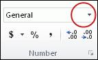
1. On the Home tab, in the Number group, click the arrow next to the list of number formats, and then click More Number Formats.

   

2. In the Category list, depending on the data type of your numbers, click Currency, Accounting, Percentage, or Scientific.

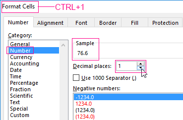
3. In the Decimal places box, enter the number of decimal places that you want to display.

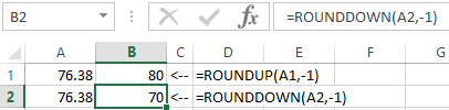
Round a number up

Use the ROUNDUP function. In some cases, you may want to use the EVEN and the ODD functions to round up to the nearest even or odd number.

Round a number down

Use the ROUNDDOWNfunction.

Round a number to the nearest number

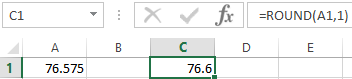
Use the ROUND function.

Round a number to a near fraction

Use the ROUND function.

Round a number to a significant digit

Significant digits are digits that contribute to the accuracy of a number.

The examples in this section use the ROUND, ROUNDUP, and ROUNDDOWN functions. They cover rounding methods for positive, negative, whole, and fractional numbers, but the examples shown represent only a very small list of possible scenarios.

The following list contains some general rules to keep in mind when you round numbers to significant digits. You can experiment with the rounding functions and substitute your own numbers and parameters to return the number of significant digits that you want.

• When rounding a negative number, that number is first converted to its absolute value (its value without the negative sign). The rounding operation then occurs, and then the negative sign is reapplied. Although this may seem to defy logic, it is the way rounding works. For example, using the ROUNDDOWN function to round -889 to two significant digits results in -880. First, -889 is converted to its absolute value of 889. Next, it is rounded down to two significant digits results (880). Finally, the negative sign is reapplied, for a result of -880.

• Using the ROUNDDOWN function on a positive number always rounds a number down, and ROUNDUP always rounds a number up.

• The ROUND function rounds a number containing a fraction as follows: If the fractional part is 0.5 or greater, the number is rounded up. If the fractional part is less than 0.5, the number is rounded down.

• The ROUND function rounds a whole number up or down by following a similar rule to that for fractional numbers; substituting multiples of 5 for 0.5.

• As a general rule, when you round a number that has no fractional part (a whole number), you subtract the length from the number of significant digits to which you want to round. For example, to round 2345678 down to 3 significant digits, you use the ROUNDDOWN function with the parameter -4, as follows: = ROUNDDOWN(2345678,-4). This rounds the number down to 2340000, with the «234» portion as the significant digits.

Round a number to a specified multiple

There may be times when you want to round to a multiple of a number that you specify. For example, suppose your company ships a product in crates of 18 items. You can use the MROUND function to find out how many crates you will need to ship 204 items. In this case, the answer is 12, because 204 divided by 18 is 11.333, and you will need to round up. The 12th crate will contain only 6 items.

There may also be times where you need to round a negative number to a negative multiple or a number that contains decimal places to a multiple that contains decimal places. You can also use the MROUND function in these cases.

You can round numbers in Excel in several ways: with helping the format of cells and with the help of functions. These two methods should be distinguished: the first only to display or print output, and the second one — for computations and calculations.

With helping functions you can accurate rounding — up or down to the user-specified discharge. And the values obtained computationally, can be used in other formulas and functions. At the same time the rounding by using the format cells does not give the desired result, and the results of calculations with these values will be erroneous. Because the format of the cells, in fact, the value does not change, the only change it its display method. To quickly and easily understand and to avoid mistakes, there are some examples.



How to round the number by the format of the cell

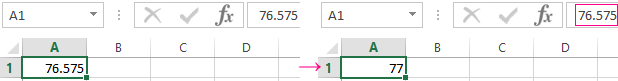
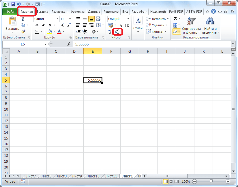
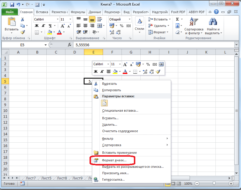
You need to put in the cell A1 the value 76. 575. Clicking with the right mouse button, we called the menu «Format of the cells» to do the same you can through the instrument of «Number» on the main page of the Book. You can also press the hot key combination CTRL+1 for this purpose.

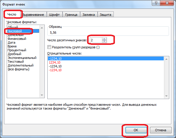
Choose the number format and set decimal places to 0.

The result of rounding:

To assign the number of decimal places we can in the «Accounting» format, «Currency», «Percentage».

Assign the number of decimal places in the «cash» format, «financial», «interest».

As we can see, the rounding occurs according to mathematical laws. The last figure which you need to keep will be increased by one, if it is followed by a figure greater than or equal to «5».

The feature of this option: the more decimal places we leave, the better the result will be got.



How to round a number in Excel

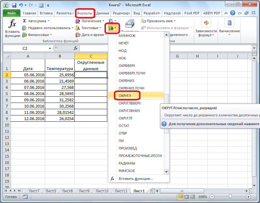
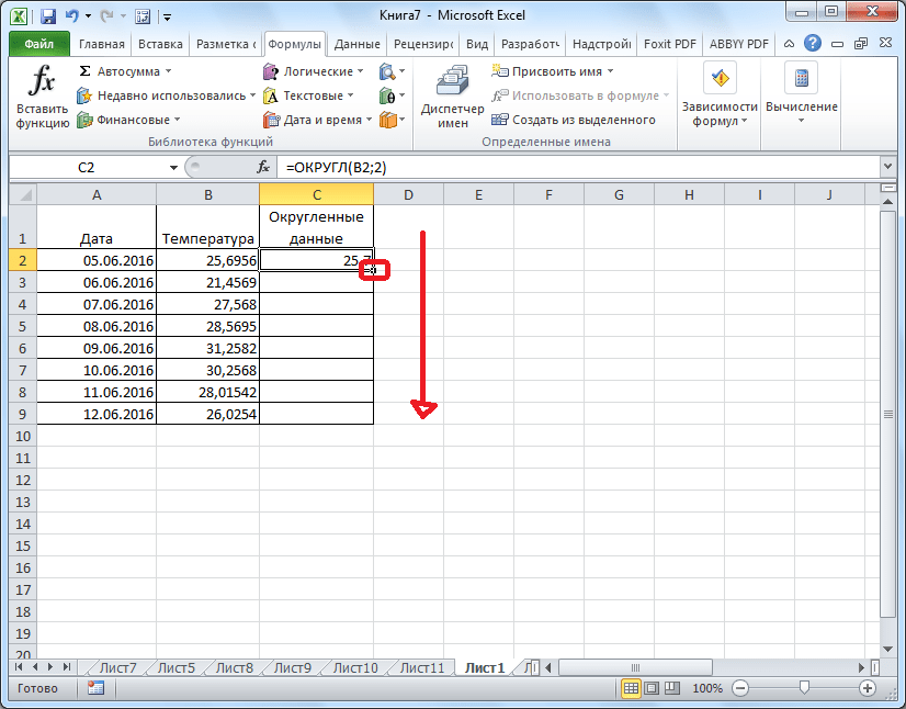
Using the function ROUND (round to user required number of decimal places). To call the «Wizards» we use the fx button. The desired function is in the category of «Mathematical».

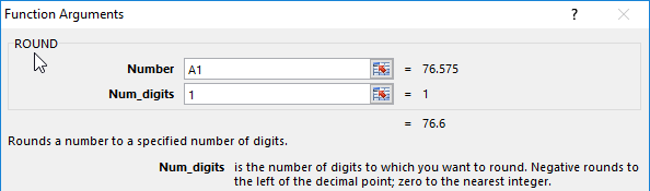
The arguments:

1. «Number» — is a reference to a cell with the desired value (A1).
2. «Number_digits» — is the value of decimal places to which you want to round (0 – to round to a whole number, 1 – it`ll be left a single decimal place, 2 – is two, etc.).

We are rounding to an integer (not a decimal) now. We use the ROUND function:

• the first argument of the function – is a reference to the cell;
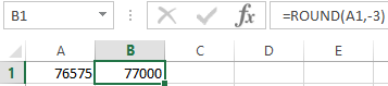
• the second argument is negative «-» (up to tens – is «-1», to hundreds – is «-2», to round a number to thousands – is «-3», etc.).

How to round a number in Excel to thousands?

The example rounding of a number to thousands:

The formula: =ROUND(A1,-3)

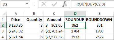
You can round up not only the number but also the value of the expression.

For example, there are findings on price and quantity of good. You need to find a value accurate to ruble (round up to the nearest whole number).

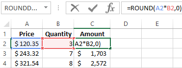
The function’s first argument — is a numeric expression for finding the value.

How to round in large and smaller side in Excel

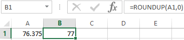
For rounding off in a big way – is the function «ROUNDUP».

The first argument we fill in on the familiar principle – is a reference to a data cell.

The second argument: «0» — round of a decimal to an integer, «1» — the function rounds, leaving one decimal place after the decimal point, etc.

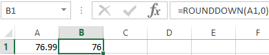
Formula: =ROUNDDOWN(A1,0)

The result:

To round down in Excel, apply the function «ROUNDDOWN».

The example of the formula: =ROUNDDOWN(A1,0).

The result:

The formulas «ROUNDUP» and «ROUNDDOWN» are used for rounding the values of the expressions (product, sum, difference, etc.).

How to round to the nearest whole number in Excel?

To round to the nearest whole in a big way we use the function «ROUNDUP». To round to an integer value in the smaller side we use the function «ROUNDDOWN». The function «ROUND» and format of cells as well allow you to round it to integer, setting the value of digits – is «0» (see above).

In Excel for rounding to the nearest whole number we also apply the function «TRUNC». It just drops the decimal places. In fact, there is no rounding applied. The formula cuts off the numbers to the assigned category.

Compare:

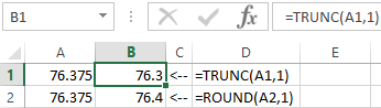
The second argument is «0» — the function cuts off to the nearest whole number; «1» — to the tenth; «2» — to the decimal places, etc.

The special Excel function, which will return only an integer – is «INT». It has the single argument. You can specify a numeric value or a cell reference.

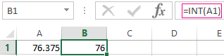
The disadvantage of using function «INT» only rounds down.

Be rounded to an integer in Excel you may using the functions «ROUNDUP» and «ROUNDDOWN». Rounding occurs up or down to the nearest of whole value.

The example of using functions:

The second argument indicates the category to which should be rounded (10 — to tens, 100 — to hundreds, etc.).

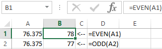
Rounding to the nearest even integer performs the function of «EVEN», to the nearest odd value — is «ODD».

The example of their using:

Why Excel rounds up large numbers?

If cells in a spreadsheet are introduced large numbers (for example, 78568435923100756), the default Excel automatically rounds down them here: 7, 85684 E + 16 – this is a feature of the format cells to «General». To avoid the display of large numbers you need to change the format of the cell with a large number of «Numerical» (the fastest way to press the hot key combination CTRL+SHIFT+1). Then the cell value will display like this: 78 568 435 923 100 756, 00. If you wish, the digit of levels can be reduced: «HOME» — «Decrease Decimal».

При выполнении деления или работе с дробными числами, Excel производит округление. Это связано, прежде всего, с тем, что абсолютно точные дробные числа редко когда бывают нужны, но оперировать громоздким выражением с несколькими знаками после запятой не очень удобно. Кроме того, существуют числа, которые в принципе точно не округляются. В то же время, недостаточно точное округление может привести к грубым ошибкам в ситуациях, где требуется именно точность. К счастью, в программе имеется возможность пользователям самостоятельно устанавливать, как будут округляться числа.

Все числа, с которыми работает Microsoft Excel, делятся на точные и приближенные. В памяти хранятся числа до 15 разряда, а отображаются до того разряда, который укажет сам пользователь. Все расчеты выполняются согласно хранимых в памяти, а не отображаемых на мониторе данных.

С помощью операции округления Эксель отбрасывает некоторое количество знаков после запятой. В нем применяется общепринятый способ округления, когда число меньше 5 округляется в меньшую сторону, а больше или равно 5 – в большую сторону.

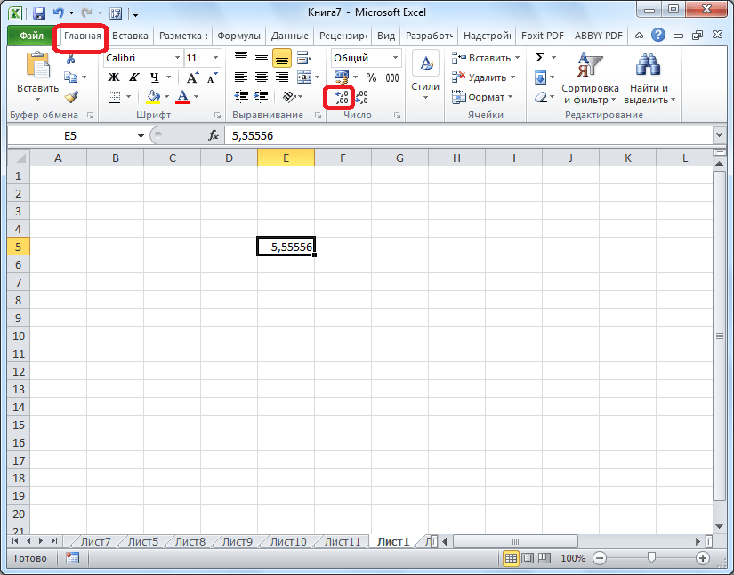
Округление с помощью кнопок на ленте

Самый простой способ изменить округление — это выделить ячейку или группу ячеек и, находясь на вкладке «Главная», нажать на ленте на кнопку «Увеличить разрядность» или «Уменьшить разрядность». Обе кнопки располагаются в блоке инструментов «Число». Будет округляться только отображаемое число, но для вычислений при необходимости будут задействованы до 15 разрядов чисел.

При нажатии на кнопку «Увеличить разрядность» количество внесенных знаков после запятой увеличивается на один.

Кнопка «Уменьшить разрядность», соответственно, уменьшает на одну количество цифр после запятой.

Округление через формат ячеек

Есть возможность также выставить округление с помощью настроек формата ячеек. Для этого нужно выделить диапазон ячеек на листе, кликнуть правой кнопкой мыши и в появившемся меню выбрать пункт «Формат ячеек».

В открывшемся окне настроек формата ячеек следует перейти на вкладку «Число». Если формат данных указан не числовой, необходимо выставить именно его, иначе вы не сможете регулировать округление. В центральной части окна около надписи «Число десятичных знаков» просто укажите цифрой то количество знаков, которое желаете видеть при округлении. После этого примените изменения.

Установка точности расчетов

Если в предыдущих случаях устанавливаемые параметры влияли только на внешнее отображения данных, а при расчетах использовались более точные показатели (до 15 знака), то сейчас мы расскажем, как изменить саму точность расчетов.

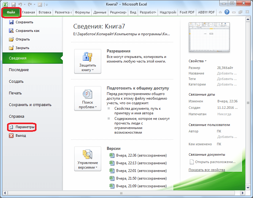
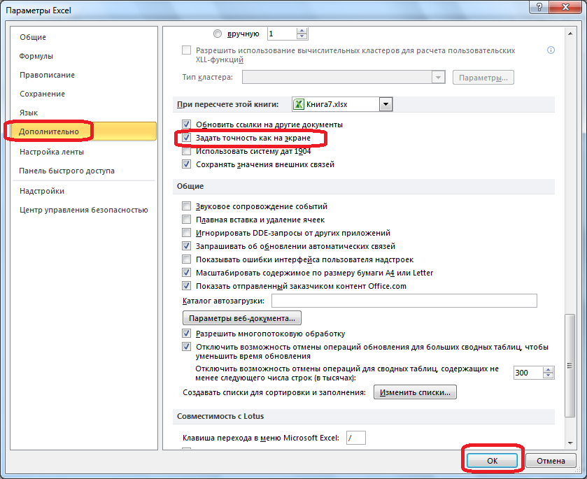
1. Перейдите на вкладку «Файл», оттуда — в раздел «Параметры».





2. Откроется окно параметров Excel. В этом окне зайдите в подраздел «Дополнительно». Отыщите блок настроек под названием «При пересчете этой книги». Настройки в этом блоке применяются не к одному листу, а к книге в целом, то есть ко всему файлу. Поставьте галочку напротив параметра «Задать точность как на экране» и нажмите «OK».



3. Теперь при расчете данных будет учитываться отображаемая величина числа на экране, а не та, которая хранится в памяти Excel. Настройку же отображаемого числа можно провести любым из двух способов, о которых мы говорили выше.

Применение функций

Если же вы хотите изменить величину округления при расчете относительно одной или нескольких ячеек, но не хотите понижать точность расчетов в целом для документа, в этом случае лучше всего воспользоваться возможностями, которые предоставляет функция «ОКРУГЛ» и различные ее вариации, а также некоторые другие функции.

Среди основных функций, которые регулируют округление, следует выделить такие:

Функция	Описание
ОКРУГЛ	Округляет до указанного числа десятичных знаков согласно общепринятым правилам округления
ОКРУГЛВВЕРХ	Округляет до ближайшего числа вверх по модулю
ОКРУГЛВНИЗ	Округляет до ближайшего числа вниз по модулю
ОКРУГЛТ	Округляет число с заданной точностью
ОКРВВЕРХ	Округляет число с заданной точностью вверх по модулю
ОКРВНИЗ	Округляет число вниз по модулю с заданной точностью
ОТБР	Округляет данные до целого числа
ЧЕТН	Округляет данные до ближайшего четного числа
НЕЧЕТН	Округляет данные до ближайшего нечетного числа

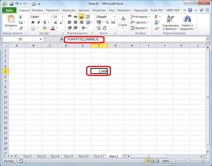
Для функций «ОКРУГЛ», «ОКРУГЛВВЕРХ» и «ОКРУГЛВНИЗ» используется следующий формат ввода: Наименование функции (число;число_разрядов). То есть если вы, к примеру, хотите округлить число 2,56896 до трех разрядов, то применяете функцию «ОКРУГЛ(2,56896;3)». В итоге получается число 2,569.

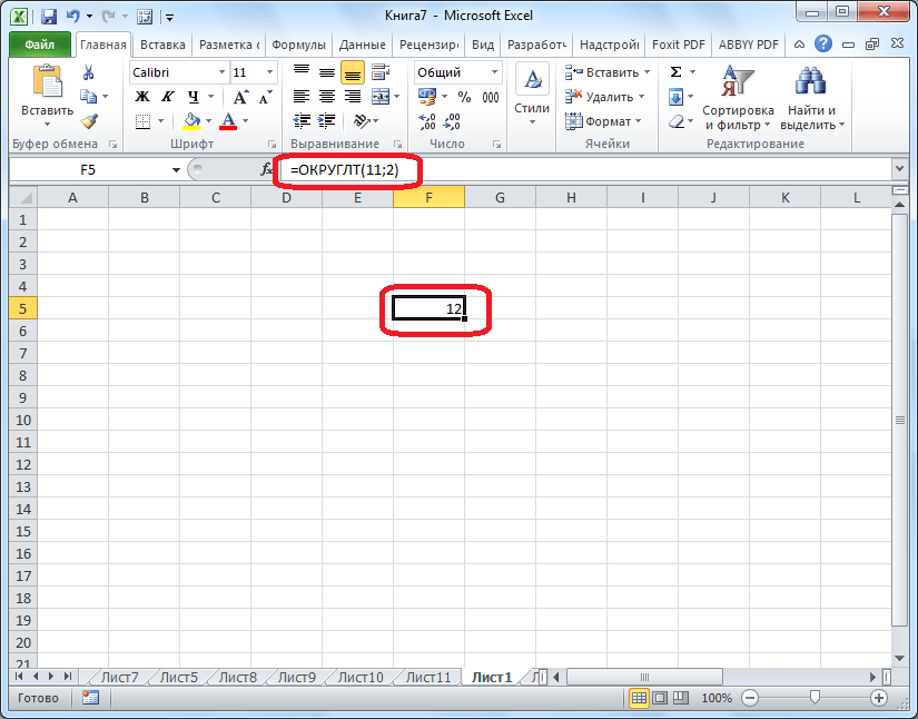
Для функций «ОКРУГЛТ», «ОКРВВЕРХ» и «ОКРВНИЗ» применяется такая формула округления: Наименование функции(число;точность). Так, чтобы округлить цифру 11 до ближайшего числа, кратного 2, вводим функцию «ОКРУГЛТ(11;2)». На выходе получается результат 12.

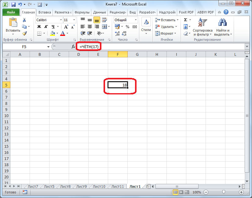
Функции «ОТБР», «ЧЕТН» и «НЕЧЕТ» используют следующий формат: Наименование функции(число). Для того чтобы округлить цифру 17 до ближайшего четного, применяем функцию «ЧЕТН(17)». Получаем результат 18.

Функцию можно вводить, как в ячейку, так и в строку функций, предварительно выделив ту ячейку, в которой она будет находиться. Перед каждой функцией следует ставить знак «=».

Существует и несколько другой способ введения функций округления. Его особенно удобно использовать, когда есть таблица со значениями, которые нужно преобразовать в округленные числа в отдельном столбике.

1. Переходим во вкладку «Формулы» и кликаем по кнопке «Математические». В открывшемся списке выбираем подходящую функцию, например, «ОКРУГЛ».



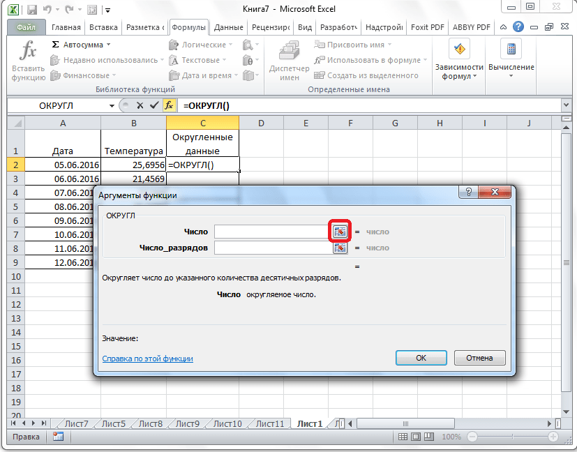
2. После этого открывается окно аргументов функции. В поле «Число» можно ввести число вручную, но если мы хотим автоматически округлить данные всей таблицы, тогда кликаем по кнопке справа от окна введения данных.



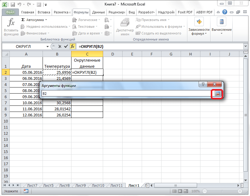
3. Окно аргументов функции сворачивается. Теперь щелкнуте по самой верхней ячейке столбца, данные которого мы собираемся округлить. После того, как значение занесено в окно, жмем по кнопке справа от этого значения.



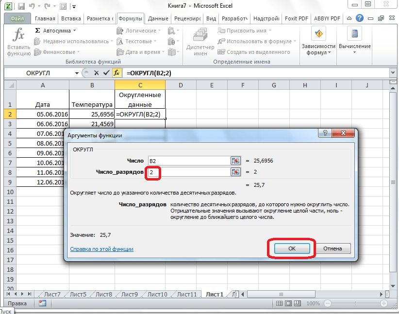
4. Опять открывается окно аргументов функции. В поле «Число разрядов» записываем разрядность, до которой нам нужно сокращать дроби и применяем изменения.



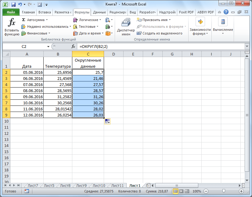
5. Число округлилось. Чтобы таким же образом округлить и все другие данные нужного столбца, наводим курсор на нижний правый угол ячейки с округленным значением, жмем на левую кнопку мыши, и протягиваем ее вниз до конца таблицы.



6. Теперь все значения в столбце будут округлены.

Как видим, существуют два основных способа округлить видимое отображение числа: с помощью кнопки на ленте и путем изменения параметров формата ячеек. Кроме того, можно изменить и округление реально рассчитываемых данных. Это также можно сделать по-разному: изменением настроек книги в целом или применением специальных функций. Выбор конкретного метода зависит от того, собираетесь ли вы применять подобный вид округления для всех данных в файле или только для определенного диапазона ячеек.

Is this article up to date?