
Excel for Microsoft 365 Excel for Microsoft 365 for Mac Excel for the web Excel 2021 Excel 2021 for Mac Excel 2019 Excel 2019 for Mac Excel 2016 Excel 2016 for Mac Excel 2013 Excel 2010 Excel 2007 Excel for Mac 2011 Excel Starter 2010 More…Less
This article describes the formula syntax and usage of the RAND function in Microsoft Excel.
Description
RAND returns an evenly distributed random real number greater than or equal to 0 and less than 1. A new random real number is returned every time the worksheet is calculated.
Syntax
RAND()
The RAND function syntax has no arguments.
Remarks
-
To generate a random real number between a and b, use:
=RAND()*(b-a)+a
-
If you want to use RAND to generate a random number but don’t want the numbers to change every time the cell is calculated, you can enter =RAND() in the formula bar, and then press F9 to change the formula to a random number. The formula will calculate and leave you with just a value.
Example
Copy the example data in the following table, and paste it in cell A1 of a new Excel worksheet. For formulas to show results, select them, press F2, and then press Enter. You can adjust the column widths to see all the data, if needed.
|
Formula |
Description |
Result |
|---|---|---|
|
=RAND() |
A random number greater than or equal to 0 and less than 1 |
varies |
|
=RAND()*100 |
A random number greater than or equal to 0 and less than 100 |
varies |
|
=INT(RAND()*100) |
A random whole number greater than or equal to 0 and less than 100 |
varies |
|
Note: When a worksheet is recalculated by entering a formula or data in a different cell, or by manually recalculating (press F9), a new random number is generated for any formula that uses the RAND function. |
Need more help?
You can always ask an expert in the Excel Tech Community or get support in the Answers community.
See Also
Mersenne Twister algorithm
RANDBETWEEN function
Need more help?
Want more options?
Explore subscription benefits, browse training courses, learn how to secure your device, and more.
Communities help you ask and answer questions, give feedback, and hear from experts with rich knowledge.
There may be cases when you need to generate random numbers in Excel.
For example, to select random winners from a list or to get a random list of numbers for data analysis or to create random groups of students in class.
In this tutorial, you will learn how to generate random numbers in Excel (with and without repetitions).
Generate Random Numbers in Excel
There are two worksheet functions that are meant to generate random numbers in Excel: RAND and RANDBETWEEN.
- RANDBETWEEN function would give you the random numbers, but there is a high possibility of repeats in the result.
- RAND function is more likely to give you a result without repetitions. However, it only gives random numbers between 0 and 1. It can be used with RANK to generate unique random numbers in Excel (as shown later in this tutorial).
Generate Random Numbers using RANDBETWEEN function in Excel
Excel RANDBETWEEN function generates a set of integer random numbers between the two specified numbers.
RANDBETWEEN function takes two arguments – the Bottom value and the top value. It will give you an integer number between the two specified numbers only.
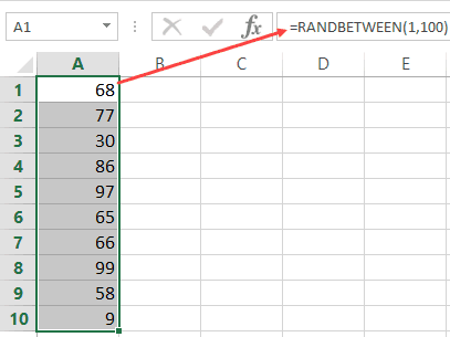
For example, suppose I want to generate 10 random numbers between 1 and 100.
Here are the steps to generate random numbers using RANDBETWEEN:
- Select the cell in which you want to get the random numbers.
- In the active cell, enter =RANDBETWEEN(1,100).
- Hold the Control key and Press Enter.
This will instantly give me 10 random numbers in the selected cells.
While RANDBETWEEN makes it easy to get integers between the specified numbers, there is a high chance of repetition in the result.
For example, when I use the RANDBETWEEN function to get 10 random numbers and use the formula =RANDBETWEEN(1,10), it gives me a couple of duplicates.
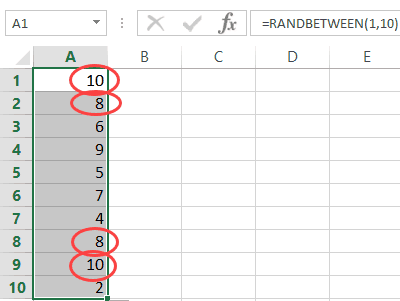
If you’re OK with duplicates, RANDBETWEEN is the easiest way to generate random numbers in Excel.
Note that RANDBETWEEN is a volatile function and recalculates every time there is a change in the worksheet. To avoid getting the random numbers recalculate, again and again, convert the result of the formula to values.
Generate Unique Random Numbers using RAND and RANK function in Excel
I tested the RAND function multiple times and didn’t find duplicate values. But as a caution, I recommend you check for duplicate values when you use this function.
Suppose I want to generate 10 random numbers in Excel (without repeats).
Here are the steps to generate random numbers in Excel without repetition:
Now you can use the values in column B as the random numbers.
Note: RAND is a volatile formula and would recalculate every time there is any change in the worksheet. Make sure you have converted all the RAND function results to values.
Caution: While I checked and didn’t find repetitions in the result of the RAND function, I still recommend you check once you have generated these numbers. You can use Conditional Formatting to highlight duplicates or use the Remove Duplicate option to get rid of it.
You May Also Like the Following Excel Tutorials:
- Automatically Sort Data in Alphabetical Order using Formula.
- Random Group Generator Template
- How to Shuffle a List of Items/Names in Excel?
- How to Do Factorial (!) in Excel (FACT function)
Rand | RandBetween | RandArray
Excel has two very useful functions when it comes to generating random numbers. RAND and RANDBETWEEN.
Rand
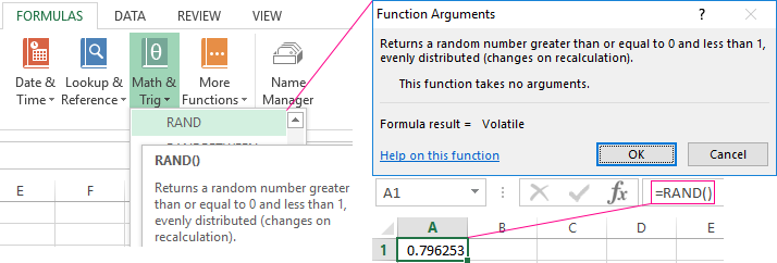
The RAND function generates a random decimal number between 0 and 1.
1. Select cell A1.
2. Type =RAND() and press Enter. The RAND function takes no arguments.

3. To generate a list of random numbers, select cell A1, click on the lower right corner of cell A1 and drag it down.

Note that cell A1 has changed. That is because random numbers change every time a cell on the sheet is calculated.
4. If you don’t want this, simply copy the random numbers and paste them as values.

5. Select cell C1 and look at the formula bar. This cell holds a value now and not the RAND function.

RandBetween
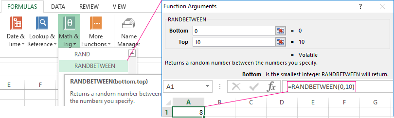
The RANDBETWEEN function generates a random whole number between two boundaries.
1. Select cell A1.
2. Type RANDBETWEEN(50,75) and press Enter.

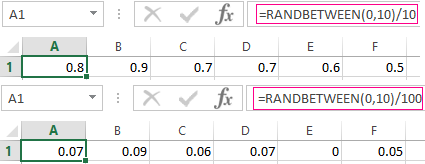
3. If you want to generate random decimal numbers between 50 and 75, modify the RAND function as follows:

RandArray
If you have Excel 365 or Excel 2021, you can use the magic RANDARRAY function.
1. By default, the RANDARRAY function generates random decimal numbers between 0 and 1. The array below consists of 5 rows and 2 columns.

Note: this dynamic array function, entered into cell A1, fills multiple cells. Wow! This behavior in Excel 365/2021 is called spilling.
2. The RANDARRAY function below generates an array of integers, 10 rows by 1 column, between 20 and 80.

Note: the Boolean TRUE (fifth argument) tells the RANDARRAY function to return an array of integers. Use FALSE to return an array of decimal numbers between 20 and 80.
We have got a sequence of numbers consisting of virtually independent elements that obey a certain counting distribution. As a rule, it’s a uniform distribution.
There are different ways to generate random numbers in Excel. Let’s view the best of them.
Random Number Function In Excel
- The function RAND() returns a random real number of a uniform distribution. It will be less than 1, and greater than or equal to 0.
- The function RANDBETWEEN returns a random integer number.
Let’s view some examples of their practical application.
Selection of random numbers using RAND
This function doesn’t require arguments.
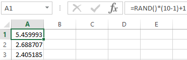
For example, to generate a random real number in the range 1 to 10, use the following formula: =RAND()*(5-1)+1.
The returned random number is distributed uniformly on the interval [1,10].
Each time the sheet is calculated or the value is changed in any cell within the sheet, a new random number is returned. If you want to save the generated set of numbers, replace the formula with its value.
- Click on the cell containing the random number.
- Select the formula in the formula bar.
- Press F9. Then Enter.
Let us check the uniformity of distribution of the random numbers from the first selection using a distribution bar chart.
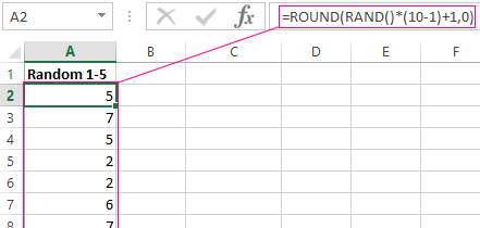
- We round the values that the function =RAND() returns. To do this, we use the function: =ROUND().And fill this formula with the big range: A2:A201.
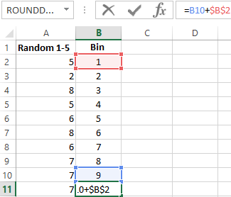
- Form the ranges to contain the values (bin). The first such range is 0-0.1. For the subsequent ones use the formula =B2+$B$2.
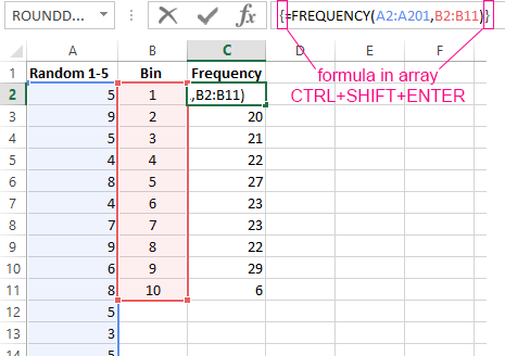
- Determine the frequency of random numbers in range A2:A201. In cell C2 use the array formula:
After input formula, select range C2:C11, press key F2 and press hot keys: CTRL+SHIFT+ENTER. We will execute the formula in the array Excel.
- Form the ranges with the use of the concatenation character (=»[0,0-«&C2&»]»).
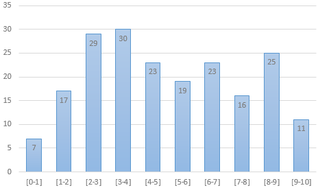
- Build a distribution bar chart for the 200 values obtained with the use of the RAND() function.
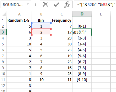
The vertical values represent the frequency. The horizontal ones represent the ranges.
RANDBETWEEN function
The syntax of the RANDBETWEEN function is as follows: (lower limit; upper limit). The first argument must be less than the second. Otherwise, the function will return an error. It is assumed that the limits are integers. The formula discards the fractional part.
An example of the function’s application:
Random numbers with an accuracy of 0.1 and 0.01:
How To Create Random Number Generator In Excel
Let’s create a random number generator that generates values from a certain range. Use a formula of the following form:
The formula randomly selects any of the numbers in the range A1:A10.
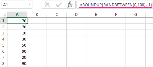
Let’s create a random number generator in the range 0-100, with a step of 10.
It’s required to select 2 random text values from the list. Using the RAND() function, let’s match the text values in the range A1:A7 with random numbers.
Use the =INDEX function to select two random text values from the initial list.
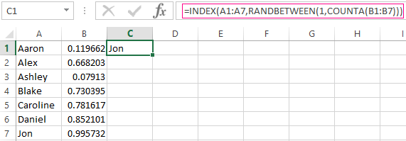
To select one random value from the list, apply the following formula:
Generator Of Standard Distribution Random Numbers
The RAND and RANDBETWEEN functions return random numbers with a single distribution. There’s an equal probability for any value to fall into the lower or upper limit of the requested range. The variation of the target value turns out to be huge.
A standard distribution means most of the generated numbers are close to the target number. Let’s adjust the RANDBETWEEN formula and create an array of data with a standard distribution.
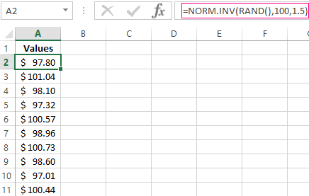
The prime cost of the X product is $100. The entire batch is subject to a standard distribution. The random variable also obeys a standard probability distribution.
Under such conditions, the average value of the range is $100. Let’s generate an array and build a chart that obeys a standard distribution with a standard deviation of $1.5.
Use the function:
Excel calculates the values in the range of probabilities. As the probability of manufacturing a product with a prime cost of $100 is maximal, the formula returns values that are close to 100 more often than other values.
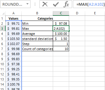
Let’s proceed to building the chart. First of all, you need to create a table containing the categories. To do this, split the array into periods:
- Determine the minimum and maximum values in the range using the =MIN(A2:102) and =MAX(A2:102) functions.
- Indicate the value of each period or step. In our example, it’s equal to 1.
- The number of categories is 10.
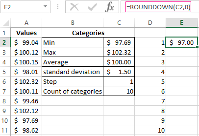
- The lower limit of the table containing the categories is the nearest multiple number rounded down. Enter the formula =ROUNDDOWN(C2,0) into the E1 cell.
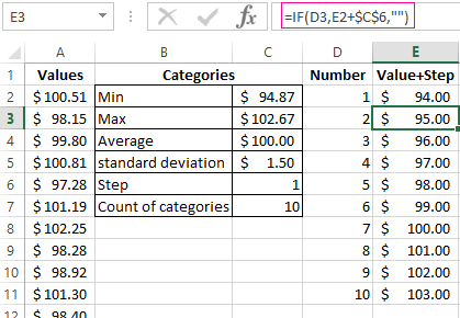
- In the E2 cell and below, the formula will look as follows:
That is, each subsequent value is increased by the specified step size.
- Let’s calculate the number of variables in the given interval. Use the function:
The formula will look as follows:
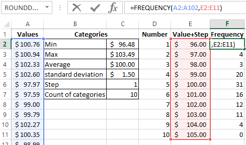
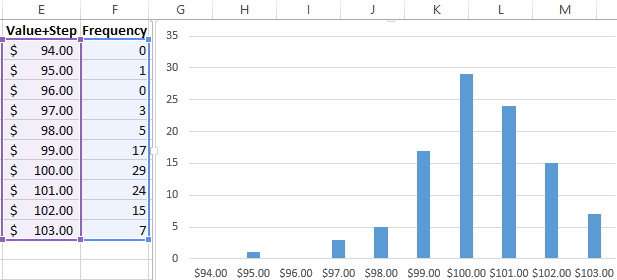
Based on the obtained data, we can build a chart with a normal distribution. The value axis represents the number of variables in the interval; the category axis represents the periods.
A chart with a normal distribution is built. As it should be, its shape resembles a bell.
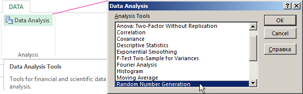
There’s a much simpler way to do the same with the help of the «Data Analysis» package. Select «Random Number Generation».
Click here to learn how to set up the standard feature: «Data Analysis».
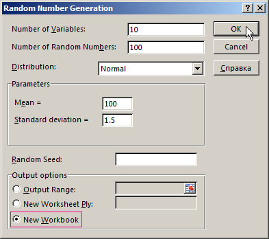
Fill in the generation parameters. Set the distribution as «Normal».
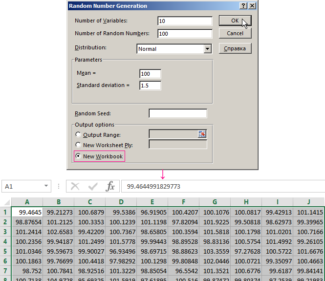
Click OK. It gives us a set of random numbers. Open the «Data Analysis» once again. Select «Histogram». Configure the parameters. Be sure to check the «Chart Output» box.
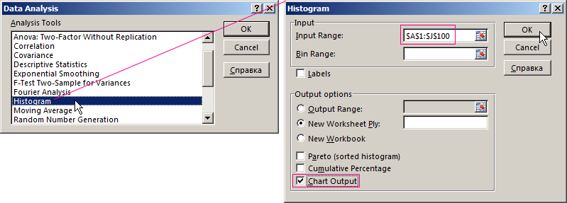
The obtained result is as follows:
Download random number generators in Excel
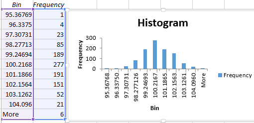
An Excel chart with a standard distribution has been built.
What Are Random Numbers In Excel?
Random numbers in Excel are used when we want to randomize our data for a sample evaluation. These numbers generated randomly. There are two built-in functions in Excel which give us random values in cells, RAND and RANDBETWEEN functions.
RAND() function provides us with any value from the range 0 to 1, whereas =RANDBETWEEN() takes input from the user for an arbitrary number range.
Randomness has many uses in science, art, statistics, cryptography, and other fields.
Generating Random numbers in excel is important because many things in real life are so complicated that they appear random. Therefore, to simulate those processes, we need random numbers.
For instance, we can generate a random number in excel using =RAND().
- Step 1: Insert the =RAND() in cell A1.

- Step 2: Press Enter.

Likewise, we can generate random numbers using random numbers in excel.
Table of contents
- What Are Random Numbers In Excel?
- How To Generate Random Numbers In Excel?
- How To Generate Random Numbers In Excel For More Than One Cell?
- RANDBETWEEN() Function
- Important Things To Remember
- Random Numbers In Excel – Project 1
- Random Numbers In Excel – Project 2 – Head And Tail
- Random Numbers In Excel – Project 3 – Region Allocation
- Random Numbers In Excel – Project 4 – Creating Ludo Dice
- Frequently Asked Questions (FAQs)
- Recommended Articles
- Random Numbers in excel is used to generate numbers in excel.
- The Random numbers in Excel function help in generating random data for sample evaluation.
- Remember, the Random Numbers in excel is a worksheet function (WS function)
- Excel has two built-in Random functions which yield random values. They are =RAND() function and =RANDBETWEEN().
- The =RAND() provides us with any value from the range 0 to 1, whereas the =RANDBETWEEN() function takes input from the user for an arbitrary number range.

You are free to use this image on your website, templates, etc, Please provide us with an attribution linkArticle Link to be Hyperlinked
For eg:
Source: Random Numbers in Excel (wallstreetmojo.com)
How To Generate Random Numbers In Excel?
There are several methods to generate a random number in Excel. We will discuss the two of them: RAND() and RANDBETWEEN() functions.
You can download this Generate Random Number Excel Template here – Generate Random Number Excel Template
#1 – RAND() Function
To generate a random number in Excel between 0 and 1(excluding), we have a RAND() function in Excel.
RAND() functions return a random decimal number that is equal to or greater than 0 but less than 1 (0 ≤ random number <1). In addition, the RAND function recalculates when a worksheet is opened or changed (volatile function).
The RAND function returns the value between 0 and 1 (excluding).
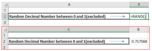
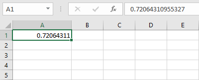
We must type =RAND() in the cell and press Enter. The value will change whenever any change is made in the sheet.
How To Generate Random Numbers In Excel For More Than One Cell?
If we want to generate random numbers in Excel for more than one cell, then we need:
- First, select the required range, type =RAND(), and press Ctrl+Enter to give us the values.
How to Stop Recalculation of Random Numbers in Excel?
As the RAND function recalculates, if any change in the sheet is made, we must copy and then paste the formulas as values if we do not want values to be changed every time. For this, we need to paste the values of the RAND() function using Paste Special so that it would no longer be a result of the “RAND ()” function. It will not be recalculated.
To do this,
- We need to make the selection of the values.
- Press the Ctrl+C keys to copy the values.

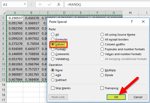
- Without changing the selection, press the Alt+Ctrl+V keys to open the Paste Special dialog box.
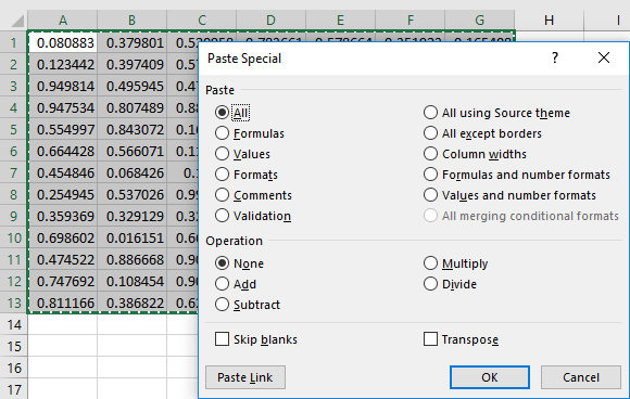
- Choose Values from the options and click on OK.
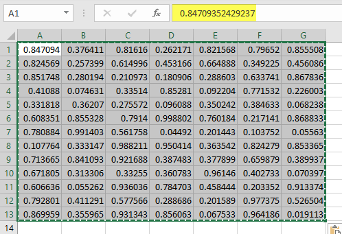
We can see that the value in the formula bar is the value itself, not the RAND() function. Now, these are only values.
There is one more way to get the value, only not the function as a result, but that is only for one cell. If we want the value the very first time, not the function, then the steps are:
- First, type =RAND() in the formula bar, press F9, and press the Enter key.
After pressing F9, we get the value only.
Value From A Different Range Other Than 0 And 1 Using RAND()
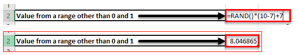
As the RAND function returns a random decimal number between 0 and 1 only, if we want the value from a different range, then we can use the following function:
Let ‘a’ be the start point.
And ‘b’ be the end point
The function would be ‘RAND()*(b-a)+a’
For example, if we have 7 as “a” and 10 as “b,” then the formula would be “=RAND()*(10-7)+7.”
RANDBETWEEN() Function
As the function’s name indicates, this function returns a random integer between given integers. Like the RAND() function, this function also recalculates when a workbook is changed or opened (volatile function).
The formula of the RANDBETWEEN Function is:
- Bottom: An integer representing the lower value of the range.
- Top: An integer representing the lower value of the range.
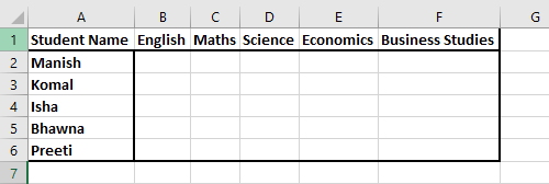
To generate random numbers in Excel for the students between 0 and 100, we will use the RANDBETWEEN function.
First, we must select the data, type the formula, =RANDBETWEEN(0,100), and press the Ctrl + Enter keys. You can prefer the below-given screenshot.
As values will recalculate, we can only use Alt+Ctrl+V to open the Paste Special dialog box to paste as values.
Follow the steps given below in the screenshot.
Like the RAND() function, we can also type the RANDBETWEEN function in the formula bar, pressing F9 to convert the result into value, and then press the Enter key.
Important Things To Remember
- If the bottom is greater than the top, the RANDBETWEEN function will return #NUM! Error.
- If either of the supplied arguments is non-numeric, the function will return #VALUE! Error.
- Both RAND() and RANDBETWEEN() functions are volatile functions (recalculates). Hence, it increases the processing time and can slow down the workbook.
Random Numbers In Excel – Project 1
We can use the RANDBETWEEN() function for getting random dates between two dates.
We will be using two dates as the bottom and top arguments.

After making the selection, we need to copy down the formula using the shortcut (Ctrl+D).

We can change the start date (D1) and end date (E1) to change the top and bottom values for the function.
Random Numbers In Excel – Project 2 – Head And Tail
To randomly choose head and tail, we can use the CHOOSE function in excel with the RANDBETWEEN function.

We need to copy the formula into the next and next cell every time in the game, and Head and Tail will come randomly.
Random Numbers In Excel – Project 3 – Region Allocation
Many times, we have to imagine and create data for various examples. For example, suppose we have data for sales, and we need to allocate three different regions to every sale transaction.
Then, we can use the RANDBETWEEN function with the CHOOSE function.

We can drag the same for the remaining cells.
Random Numbers In Excel – Project 4 – Creating Ludo Dice
Using the RANDBETWEEN function, we can also create dice for Ludo. We need to use the RANDBETWEEN function in Excel VBA for the same. Please follow the below steps:
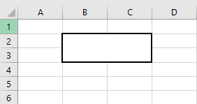
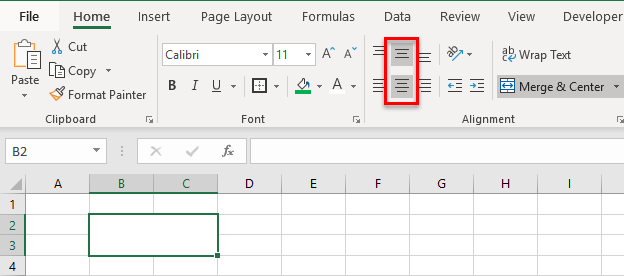
- Merge the four cells (B2:C3) using Home Tab → Alignment Group → Merge & Center.
- Apply the border to the merged cell using the shortcut key (ALT+H+B+T) by pressing one key after another.
- Center and middle align the value using Home Tab → Alignment Group → Center and Middle Align commands.
- To create the button, use Developer tab → Controls Group → Insert → Command Button
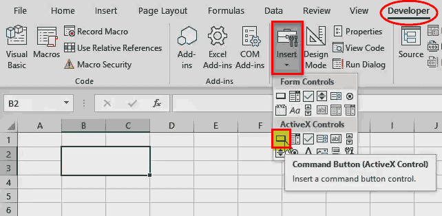
- Create the button and choose View Code from the Controls group on Developer.

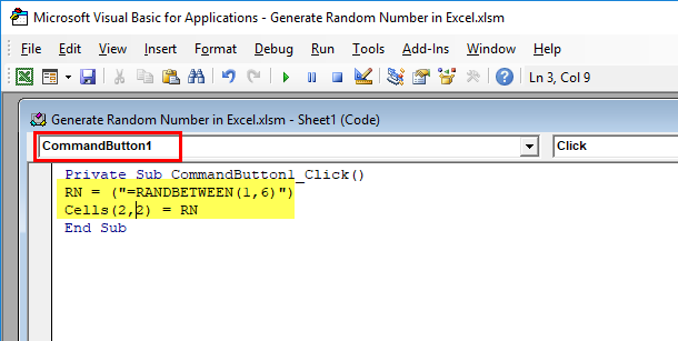
- After choosing CommandButton1 from the dropdown, paste the following code:
RN = (“=RANDBETWEEN(1,6)”)
Cells(2, 2) = RN
Please save the file using the .xlsm extension as we have used the VBA code in the workbook. After coming to the Excel window, deactivate the Design Mode.
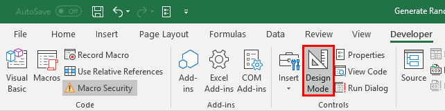
Now, whenever we click the button, we get a random value between 1 and 6.
Frequently Asked Questions (FAQs)
1. What is Random Numbers in excel?
Random Numbers in excel is a built-in function used to generate random values. It is used when we have to calculate sample evaluation for random values.
2. What are the two functions used to generate random numbers in excel?
In excel, we can generate numbers using two functions. They are: =RAND() and =RANDBETWEEN().
The =RAND() provides us with any value from the range 0 to 1, whereas the =RANDBETWEEN() function takes input from the user for an arbitrary number range.
3. How to use RAND function in excel?
RAND() generates random numbers between 0 to 1.
For example, consider the below image where we have inserted the RAND() in a blank cell.

As soon as we press Enter¸ we can see that the function has generated a random number below 1 as shown in the below image.

Similarly, we can generate random numbers between 0 to 1, using random numbers in excel function.
Recommended Articles
This article is a guide to Random Numbers in Excel. Here, we discuss generating random numbers in Excel using the RAND() and RANDBETWEEN functions along with multiple projects and downloadable Excel templates. You may also look at these useful functions in Excel: –
- Randomize List in Excel
- Auto Number in Excel
- VBA Random Number
- RAND Function in Excel
Organizing is good but sometimes a measure of randomness makes things better. That is true for life and Excel and we are here for the Excel side of matters. Excel is quite proficient with sorting lists; alphabetical order, chronological order, ascending and descending order but it’s yet to come up with straight-up randomization (nearly oxymoron-ish). Although we do have functions to help us along with that and that’s what we will be looking up in a bit.
You may want to randomize a list of names of students, employees, contestants, etc. just to prevent tipping the balance that comes from good old alphabetical sorting. You might want to rearrange dates or scramble a list of names or products. Or maybe you’re just randomly aiming to be an Excel nerd.
This tutorial will teach you how to randomize a list in Excel using functions alone and also with the Excel Sort & Filter feature. While we’re at it, you’ll also learn to use functions to make a random pick from the list.
 1")
For our example to be used throughout this guide, we will randomize the following list of names that are arranged in an alphabetical order:
 2")
Let’s start exploring the options and see what we can do to randomize lists.
Using RAND Function & Sort Feature to Randomize a List
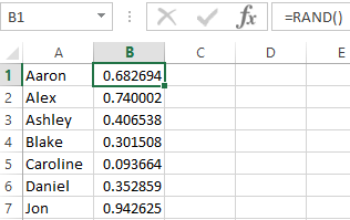
We can’t randomly sort names but we can have an arrangement of random numbers. This is where we will utilize the RAND function. The RAND function returns a random number greater than 0 and less than 1. We will get a list of random numbers lined up with the names and then sort them using the Sort & Filter tool which will then have the names randomly scrambled. Let us show you the steps.
- Enter the RAND function against the first name in a new column. This is the formula you need to enter:
=RAND()
 3")
- This formula is simply the RAND function applied on its own with no arguments. The RAND function returns random values that are greater than 0 but less than 1.
- Select and drag the formula.
 4")
- Select any cell containing the number. Navigate to the Home tab > Editing group, select the Sort & Filter option. From the drop-down, select either of the top two options. We will go with the first one – Sort Smallest to Largest.
 5")
- This will rearrange the names to be randomly jumbled. The numbers will recalculate (which is a part of random functions) and not to worry, since you won’t be needing them much longer.
 6")
- Now that we have our random list ready, we can select the column with the RAND function and delete it.
 7")
Notes:
We mentioned in the steps that recalculation of the numbers is a part of random functions. By that, we mean the RAND is a volatile function and for all volatile functions, Excel triggers recalculation on every worksheet change. This means you can keep scrambling the data (names in this case) using the Sort & Filter tool until the randomness is good to go.
The data in any columns aligned with the RAND function column will also rearrange linearly. Even if there are columns on both sides of the RAND function column, they will all rearrange linearly together.
The upside of this method is that you keep the original list and randomize that instead of creating a new list from the original as a base.
Using RANDBETWEEN Function & Sort Feature to Randomize a List
Not very different from the method above – we’re only switching things up here, swapping the RAND function for the RANDBETWEEN function. The RANDBETWEEN function returns a random number between the specified range.
First, we will use the RANDBETWEEN function to return random numbers against our list of names. Then, we will use the Sort & Filter tool to rearrange those random numbers, which will also rearrange our list of names into a randomized list. We have the steps as follows:
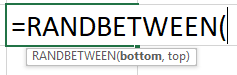
- In the column next to the names, enter the following formula for the RANDBETWEEN function:
=RANDBETWEEN(1,10)
 8")
- In this formula, we use the RANDBETWEEN function to return a random number from 1 to 10.
- Select any cell from the range and navigate to the Home tab > Editing group > Sort & Filter button > Sort Smallest to Largest (any of the two options will work).
 9")
- This will rearrange the names to be randomly jumbled. The numbers will recalculate (RANDBETWEEN too is a volatile function) which is not an issue since you will be deleting the numbers soon.
 10")
- Now that we have our random list ready, we can select the column with the RANDBETWEEN function and delete it.
 11")
Using RANDARRAY, SORTBY, & ROWS Functions to Randomize a List
Using a base list, a randomized list can be created using the RANDARRAY, SORTBY, and ROWS Functions. The RANDARRAY function returns an array of random numbers. The SORTBY function sorts a range based on the values in a corresponding range. The ROWS function returns the number of rows in a reference.
For the formula we will use, the ROWS function will return the number of rows for RANDARRAY to randomize. Then the SORTBY function will sort the list according to the randomized rows.
Let’s see how all of this looks on a sheet. Enter the following formula in a separate column:
=SORTBY(B3:B12,RANDARRAY(ROWS(B3:B12)))
 12")
The ROW function returns the number of rows in B3:B12 which is 10. The RANDARRAY function takes that number and returns an array of 10 random numbers for all 10 rows. Then the SORTBY function sorts B3:B12 according to the randomized numbers which randomly adjusts B3:12 into a new list.
This is quite like the two methods above without having a separate column for random numbers.
There is no need to make the list of names into absolute references in the formula. There is also no need to drag the formula since the results of this formula spill to create the randomized list.
Select the new randomized column, and copy-paste the values on themselves or in a new column to avoid #REF errors when the original column is deleted. Delete rest of the data which is not needed anymore.
 13")
All three methods mentioned up until now are good if you do not want to duplicate values in your finished randomized list.
Recommended Reading: How to count non-blank cells from a list
Using INDEX and RANDBETWEEN Functions to Randomize a List
A randomized list can be created using the INDEX and RANDBETWEEN functions. Before you decide to proceed with this method, there will most probably be a repetition of values (repetitions of names in this case). If that is not an issue, let’s continue.
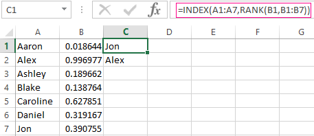
The INDEX function returns a value or its cell reference at the intersection of a particular row and column in a given range. The RANDBETWEEN function returns a random number between the specified range. In our formula, the INDEX function will work to return the value of the cell that RANDBETWEEN randomly specifies.
Let’s crack on with the sheets. Enter the following formula in a separate column:
=INDEX($B$3:$B$12,RANDBETWEEN(1,10),1)
You can use this formula for a single selection:
 14")
Or you can drag the formula for a randomized list:
 15")
The RANDBETWEEN function randomly returns a number from 1 to 10. In the first case, the random number generated is 4. This result is fed to the INDEX function in place of a row number. This means that the INDEX function is set to return the 4th value from the range B3:B12 which in the first instance is “Elton Schon”.
“1” at the end of the formula is not really required here but is useful if the range-fed into the formula is for a table (multiple columns) instead of a list (single column). This number signifies the column number from which the result is to be picked.
The formula has been dragged to fill the rest of the column.
Select the new randomized column, and copy-paste the values on themselves or in a new column to stop the column values from recalculating. Delete the rest of the data not needed anymore.
 16")
Notes:
For randomizing a list this way, the values will repeat. That is because of the nature of the RANDBETWEEN function randomly returning a number from the specified range. This way, each result is mutually exclusive and so the numbers can (and do) repeat.
There are a few tweaks that you can make using the RANDBETWEEN function for a randomized list without duplicates, adding more functions into the works but that would make the process lengthier and unnecessarily complicated when there are other methods that get the work done in much simpler ways. If repetitions are not an issue, then this method is alright to go with and is well suited for a single random pick too.
Also, since RANDBETWEEN function is a volatile function so its value gets recalculated on every worksheet change. This means you can keep scrambling the data (names in this case) until the randomness is good to go.
Using CHOOSE and RANDBETWEEN Functions to Randomize a List
Similar to the above method we can also generate a randomized list using the CHOOSE and RANDBETWEEN functions. A heads-up on this method; the results (names in this case) are most likely to repeat.
If that’s alright, then keep reading.
The CHOOSE function chooses a value from a list of values based on an index number. The RANDBETWEEN function returns a random number between the specified range. In our formula, the CHOOSE function will choose a name from the list of names according to the number that RANDBETWEEN randomly specifies.
Time for working the sheets. Enter the following formula in a separate column:
=CHOOSE(RANDBETWEEN(1,10),$B$3,$B$4,$B$5,$B$6,$B$7,$B$8,$B$9,$B$10,$B$11,$B$12)
You can use this formula for a single selection:
 17")
Or you can drag the formula for a randomized list:
 18")
The RANDBETWEEN function randomly returns a number from 1 to 10. In the first instance, the random number generated 3. The CHOOSE function then selects the 3rd value from the list of values fed into the function. The final result is “Bruce Grimm Dean”.
The formula has been dragged to fill the rest of the column. The list’s cell references are entered as absolute references in the formula so that the references don’t change as the formula is dragged.
Select the new randomized column, and copy-paste the values on themselves or in a new column to stop the column values from recalculating. Delete the rest of the data which is not needed anymore.
 19")
Notes:
Similar to the INDEX and RANDBETWEEN method, this method also can cause the values to repeat because of the nature of the RANDBETWEEN function. So make sure to only use it when having repetitions in the list is not an issue.
Here we come to a not-so-random end of this tutorial. We hope to have delved enough into the ways of randomizing a list in Excel to give you a good grasp of what works for your Excel situation. We will be back with more how-tos and all-about on everything in Excel. Feel free to come back for more problem-solving!
![]()
Download Article
![]()
Download Article
- Assembling the Data
- Creating a Random Sample
- Sorting the Sample
- Q&A
- Tips
- Warnings
|
|
|
|
|
This wikiHow teaches you how to generate a random selection from pre-existing data in Microsoft Excel. Random selections are useful for creating fair, non-biased samples of your data collection.
-

1
Open the Microsoft Excel program. You can also open an existing Microsoft Excel document if you have one that correlates to your random sample needs.
-
2
Select Blank workbook. If you aren’t opening a new document, skip this step.
Advertisement
-
3
Enter your data. To do this, click on a cell into which you wish to input data, then type in your data.
- Depending on the type of data you have, this process will vary. However, you should start all data in the «A» column.
- For example: you might place your users’ names in the «A» column and their responses to a survey (e.g., «yes» or «no») in the «B» column.
-
4
Make sure you have all relevant data entered into your spreadsheet. Once you’re positive that you’ve added all necessary data, you’re ready to generate your random sample.


Advertisement
-
1
Right-click the far left column’s name. For example, if all of your data begins in column «A», you’d right-click the «A» at the top of the page.
-
2
Click Insert. This will add a column to the left of your current left column.
- After doing this, any data that was in the «A» column will be relisted as being in the «B» column and so on.
-
3
Select the new «A1» cell.
-
4
Type «= RAND()» into this cell. Exclude the quotation marks. The «RAND» command applies a number between 0 and 1 to your selected cell.
- If Excel attempts to automatically format your «RAND» command, delete the formatting and re-type the command.
-
5
Press ↵ Enter. You should see a decimal (e.g., 0.5647) appear in your selected cell.
-
6
Select the cell with the random sample number.
-
7
Hold down Control and tap C. Doing this will copy the «RAND» command.
- For a Mac, you’ll hold down ⌘ Command instead of Control.
- You can also right-click the «RAND» cell and then select Copy.
-
8
Select the cell below your random sample number. This will likely be the «A2» cell.
- Clicking the «A1» cell and highlighting from there can cause a sorting error.
-
9
Highlight the rest of the random sample cells. To do this, you’ll hold down ⇧ Shift while clicking the cell at the bottom of your data range.
- For example, if your data in columns «B» and «C» extends all the way down to cell 100, you would hold down ⇧ Shift and click «A100» to select all «A» cells from A2 to A100.
-
10
Hold down Control and tap V. Doing so will paste the random sample command into all selected cells (e.g., A2 through A100). Once this is done, you’ll need to sort your data using the random numbers to reorder your results.
- Again, Mac users will need to hold down ⌘ Command instead of Control.


Advertisement
-
1
Select the top left cell. In most cases, this will be the «A1» cell. Before you can sort your sample, you’ll need to highlight all of your data.
- This includes the random sample numbers to the left of your data as well.
-
2
Hold down ⇧ Shift and select the bottom right cell. Doing so will highlight all of your data, making it ready for sorting.
- For example, if your data takes up two columns of 50 cells each, you would select «C50» while holding down ⇧ Shift.
- You can also click and drag your cursor from the top left corner to the bottom right corner of your data (or vice versa) to highlight it.
-
3
Right-click your data. This will bring up a context menu with options that will allow you to sort your data.
- If you’re using a Mac, you can click using two fingers (or hold down Ctrl and click) to bring up the context menu.
-
4
Hover your cursor over Sort.
-
5
Click Sort Smallest to Largest. You can also click Sort Largest to Smallest here—the only thing that matters is that your data is reorganized randomly according to the «= RAND()» values in the «A» column.
-
6
Review the sorting results. Depending on how many results you need, your process from here will vary. However, you can do a couple of things with the sorted data:
- Select the first, last, or middle half of the data. If your number of data points is too large to warrant this, you can also settle on a lower fraction (for example, the first eighth of the data).
- Select all odd- or even-numbered data. For example, in a set of 10 data points, you would either pick numbers 1, 3, 5, 7, and 9, or 2, 4, 6, 8, and 10.
- Select a number of random data points. This method works best for large sets of data where picking half of the information is too ambitious.
-
7
Choose your random sample participants. Now you have a non-biased sample pool for a survey, product giveaway, or something similar.


Advertisement
Add New Question
-
Question
When I copy the random values from column A and paste them in column B following the paste special -> values instruction, I get a different set of numbers from what I have in column A. Is this correct?

The values in column B should match what was in column A before, but as you paste them, the values in column A will change. That’s expected since the RAND() formula recalculates a new random number each time you do anything else in the spreadsheet. Copying the values only (not the formula) over to column B will prevent them from changing in future.
Ask a Question
200 characters left
Include your email address to get a message when this question is answered.
Submit
Advertisement
-
If you don’t have Microsoft Excel, there are other free programs online (such as Google Sheets or Outlook’s Excel app) that may allow you to create a random sample.
-
Microsoft makes an Excel app for iPhone and Android platforms so you can create spreadsheets on-the-go.
Thanks for submitting a tip for review!
Advertisement
-
Failing to use a random sample when looking for results (e.g., sending out a survey after updating a service) may cause your answers to be biased—and, therefore, inaccurate.
Advertisement
About This Article
Thanks to all authors for creating a page that has been read 442,477 times.