
Suppose that your boss wants you to protect an entire workbook, but also wants to be able to change a few cells after you enable protection on the workbook. Before you enabled password protection, you had unlocked some cells in the workbook. Now that your boss is done with the workbook, you can lock these cells.
Follow these steps to lock cells in a worksheet:
-
Select the cells you want to lock.
-
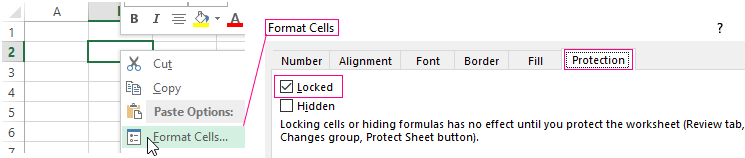
On the Home tab, in the Alignment group, click the small arrow to open the Format Cells popup window.
-
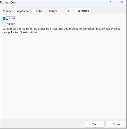
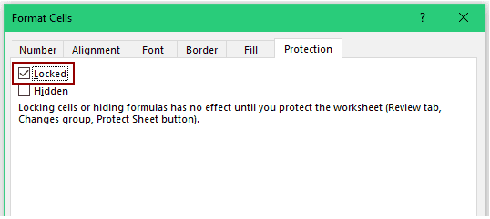
On the Protection tab, select the Locked check box, and then click OK to close the popup.
Note: If you try these steps on a workbook or worksheet you haven’t protected, you’ll see the cells are already locked. This means that the cells are ready to be locked when you protect the workbook or worksheet.
-
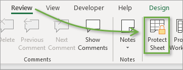
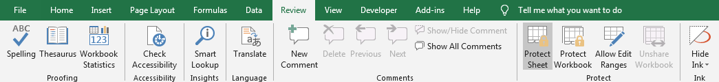
On the Review tab in the ribbon, in the Changes group, select either Protect Sheet or Protect Workbook, and then reapply protection. See Protect a worksheet or Protect a workbook.
Tip: It’s a best practice to unlock any cells that you may want to change before you protect a worksheet or a workbook, but you can also unlock them after you apply protection. To remove protection, simply remove the password.
In addition to protecting workbooks and worksheets, you can also protect formulas.
Excel for the web can’t lock cells or specific areas of a worksheet.
If you want to lock cells or protect specific areas, click Open in Excel and lock cells to protect them or lock or unlock specific areas of a protected worksheet.
By default, protecting a worksheet locks all cells so none of them are editable. To enable some cell editing, while leaving other cells locked, it’s possible to unlock all the cells. You can lock only specific cells and ranges before you protect the worksheet and, optionally, enable specific users to edit only in specific ranges of a protected sheet.
Lock only specific cells and ranges in a protected worksheet
Follow these steps:
-
If the worksheet is protected, do the following:
-
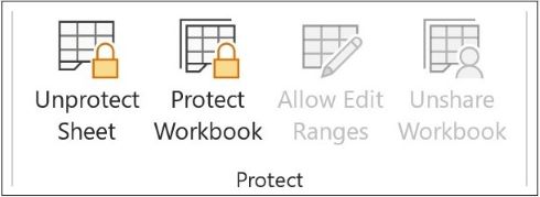
On the Review tab, click Unprotect Sheet (in the Changes group).

Click the Protect Sheet button to Unprotect Sheet when a worksheet is protected.
-
If prompted, enter the password to unprotect the worksheet.
-
-
Select the whole worksheet by clicking the Select All button.
-
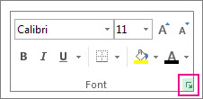
On the Home tab, click the Format Cell Font popup launcher. You can also press Ctrl+Shift+F or Ctrl+1.
-
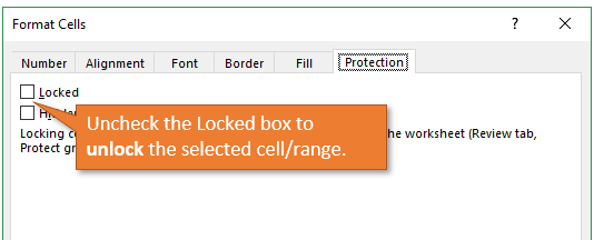
In the Format Cells popup, in the Protection tab, uncheck the Locked box and then click OK.
This unlocks all the cells on the worksheet when you protect the worksheet. Now, you can choose the cells you specifically want to lock.
-
On the worksheet, select just the cells that you want to lock.
-
Bring up the Format Cells popup window again (Ctrl+Shift+F).
-
This time, on the Protection tab, check the Locked box and then click OK.
-
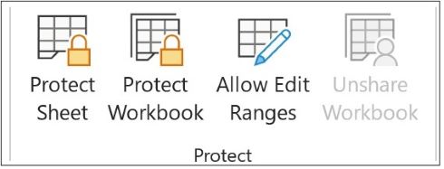
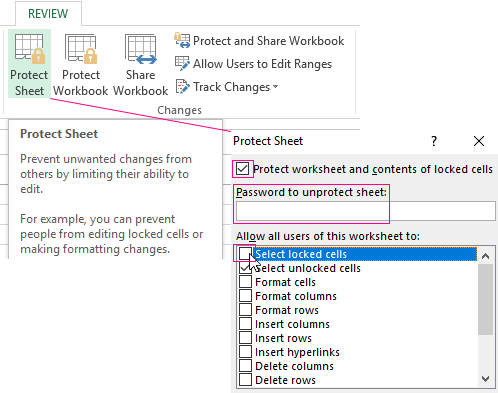
On the Review tab, click Protect Sheet.
-
In the Allow all users of this worksheet to list, choose the elements that you want users to be able to change.
More information about worksheet elements
Clear this check box
To prevent users from
Select locked cells
Moving the pointer to cells for which the Locked check box is selected on the Protection tab of the Format Cells dialog box. By default, users are allowed to select locked cells.
Select unlocked cells
Moving the pointer to cells for which the Locked check box is cleared on the Protection tab of the Format Cells dialog box. By default, users can select unlocked cells, and they can press the TAB key to move between the unlocked cells on a protected worksheet.
Format cells
Changing any of the options in the Format Cells or Conditional Formatting dialog boxes. If you applied conditional formats before you protected the worksheet, the formatting continues to change when a user enters a value that satisfies a different condition.
Format columns
Using any of the column formatting commands, including changing column width or hiding columns (Home tab, Cells group, Format button).
Format rows
Using any of the row formatting commands, including changing row height or hiding rows (Home tab, Cells group, Format button).
Insert columns
Inserting columns.
Insert rows
Inserting rows.
Insert hyperlinks
Inserting new hyperlinks, even in unlocked cells.
Delete columns
Deleting columns.
If Delete columns is protected and Insert columns is not also protected, a user can insert columns that he or she cannot delete.
Delete rows
Deleting rows.
If Delete rows is protected and Insert rows is not also protected, a user can insert rows that he or she cannot delete.
Sort
Using any commands to sort data (Data tab, Sort & Filter group).
Users can’t sort ranges that contain locked cells on a protected worksheet, regardless of this setting.
Use AutoFilter
Using the drop-down arrows to change the filter on ranges when AutoFilters are applied.
Users cannot apply or remove AutoFilters on a protected worksheet, regardless of this setting.
Use PivotTable reports
Formatting, changing the layout, refreshing, or otherwise modifying PivotTable reports, or creating new reports.
Edit objects
Doing any of the following:
-
Making changes to graphic objects including maps, embedded charts, shapes, text boxes, and controls that you did not unlock before you protected the worksheet. For example, if a worksheet has a button that runs a macro, you can click the button to run the macro, but you cannot delete the button.
-
Making any changes, such as formatting, to an embedded chart. The chart continues to be updated when you change its source data.
-
Adding or editing comments.
Edit scenarios
Viewing scenarios that you have hidden, making changes to scenarios that you have prevented changes to, and deleting these scenarios. Users can change the values in the changing cells, if the cells are not protected, and add new scenarios.
Chart sheet elements
Select this check box
To prevent users from
Contents
Making changes to items that are part of the chart, such as data series, axes, and legends. The chart continues to reflect changes made to its source data.
Objects
Making changes to graphic objects — including shapes, text boxes, and controls — unless you unlock the objects before you protect the chart sheet.
-
-
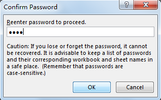
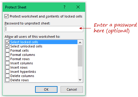
In the Password to unprotect sheet box, type a password for the sheet, click OK, and then retype the password to confirm it.
-
The password is optional. If you do not supply a password, any user can unprotect the sheet and change the protected elements.
-
Make sure that you choose a password that is easy to remember, because if you lose the password, you won’t have access to the protected elements on the worksheet.
-

Unlock ranges on a protected worksheet for users to edit
To give specific users permission to edit ranges in a protected worksheet, your computer must be running Microsoft Windows XP or later, and your computer must be in a domain. Instead of using permissions that require a domain, you can also specify a password for a range.
-
Select the worksheet that you want to protect.
-
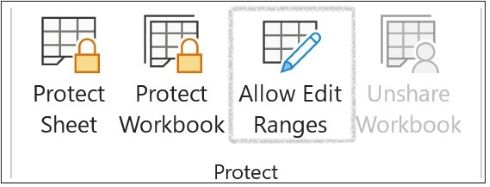
On the Review tab, in the Changes group, click Allow Users to Edit Ranges.
This command is available only when the worksheet is not protected.
-
Do one of the following:
-
To add a new editable range, click New.
-
To modify an existing editable range, select it in the Ranges unlocked by a password when sheet is protected box, and then click Modify.
-
To delete an editable range, select it in the Ranges unlocked by a password when sheet is protected box, and then click Delete.
-
-
In the Title box, type the name for the range that you want to unlock.
-
In the Refers to cells box, type an equal sign (=), and then type the reference of the range that you want to unlock.
You can also click the Collapse Dialog button, select the range in the worksheet, and then click the Collapse Dialog button again to return to the dialog box.
-
For password access, in the Range password box, type a password that allows access to the range.
Specifying a password is optional when you plan to use access permissions. Using a password allows you to see user credentials of any authorized person who edits the range.
-
For access permissions, click Permissions, and then click Add.
-
In the Enter the object names to select (examples) box, type the names of the users who you want to be able to edit the ranges.
To see how user names should be entered, click examples. To verify that the names are correct, click Check Names.
-
Click OK.
-
To specify the type of permission for the user who you selected, in the Permissions box, select or clear the Allow or Deny check boxes, and then click Apply.
-
Click OK two times.
If prompted for a password, type the password that you specified.
-
In the Allow Users to Edit Ranges dialog box, click Protect Sheet.
-
In the Allow all users of this worksheet to list, select the elements that you want users to be able to change.
More information about the worksheet elements
Clear this check box
To prevent users from
Select locked cells
Moving the pointer to cells for which the Locked check box is selected on the Protection tab of the Format Cells dialog box. By default, users are allowed to select locked cells.
Select unlocked cells
Moving the pointer to cells for which the Locked check box is cleared on the Protection tab of the Format Cells dialog box. By default, users can select unlocked cells, and they can press the TAB key to move between the unlocked cells on a protected worksheet.
Format cells
Changing any of the options in the Format Cells or Conditional Formatting dialog boxes. If you applied conditional formats before you protected the worksheet, the formatting continues to change when a user enters a value that satisfies a different condition.
Format columns
Using any of the column formatting commands, including changing column width or hiding columns (Home tab, Cells group, Format button).
Format rows
Using any of the row formatting commands, including changing row height or hiding rows (Home tab, Cells group, Format button).
Insert columns
Inserting columns.
Insert rows
Inserting rows.
Insert hyperlinks
Inserting new hyperlinks, even in unlocked cells.
Delete columns
Deleting columns.
If Delete columns is protected and Insert columns is not also protected, a user can insert columns that he or she cannot delete.
Delete rows
Deleting rows.
If Delete rows is protected and Insert rows is not also protected, a user can insert rows that he or she cannot delete.
Sort
Using any commands to sort data (Data tab, Sort & Filter group).
Users can’t sort ranges that contain locked cells on a protected worksheet, regardless of this setting.
Use AutoFilter
Using the drop-down arrows to change the filter on ranges when AutoFilters are applied.
Users cannot apply or remove AutoFilters on a protected worksheet, regardless of this setting.
Use PivotTable reports
Formatting, changing the layout, refreshing, or otherwise modifying PivotTable reports, or creating new reports.
Edit objects
Doing any of the following:
-
Making changes to graphic objects including maps, embedded charts, shapes, text boxes, and controls that you did not unlock before you protected the worksheet. For example, if a worksheet has a button that runs a macro, you can click the button to run the macro, but you cannot delete the button.
-
Making any changes, such as formatting, to an embedded chart. The chart continues to be updated when you change its source data.
-
Adding or editing comments.
Edit scenarios
Viewing scenarios that you have hidden, making changes to scenarios that you have prevented changes to, and deleting these scenarios. Users can change the values in the changing cells, if the cells are not protected, and add new scenarios.
Chart sheet elements
Select this check box
To prevent users from
Contents
Making changes to items that are part of the chart, such as data series, axes, and legends. The chart continues to reflect changes made to its source data.
Objects
Making changes to graphic objects — including shapes, text boxes, and controls — unless you unlock the objects before you protect the chart sheet.
-
-
In the Password to unprotect sheet box, type a password, click OK, and then retype the password to confirm it.
-
The password is optional. If you do not supply a password, then any user can unprotect the worksheet and change the protected elements.
-
Ensure that you choose a password that you can remember. If you lose the password, you will be unable to access to the protected elements on the worksheet.
-
If a cell belongs to more than one range, users who are authorized to edit any of those ranges can edit the cell.
-
If a user tries to edit multiple cells at once and is authorized to edit some but not all of those cells, the user will be prompted to edit the cells one-by-one.
Need more help?
You can always ask an expert in the Excel Tech Community or get support in the Answers community.
Bottom Line: Learn how to lock individual cells or ranges in Excel so that users cannot change the formulas or contents of protected cells. Plus a few bonus tips to save time with the setup.
Skill Level: Beginner
Video Tutorial
Download the Excel File
You can download the file that I use in the video tutorial by clicking below.
Protecting Your Work from Unwanted Changes
If you share your spreadsheets with other users, you’ve probably found that there are specific cells you don’t want them to modify. This is especially true for cells that contain formulas and special formatting.
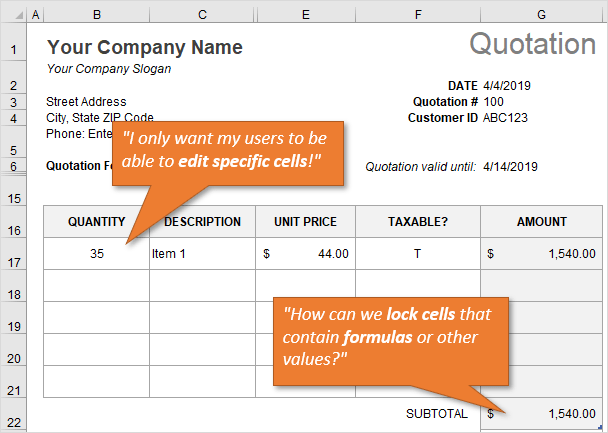
The great news is that you can lock or unlock any cell, or a whole range of cells, to keep your work protected. It’s easy to do, and it involves two basic steps:
- Locking/unlocking the cells.
- Protecting the worksheet.
Here’s how to prevent users from changing some cells.
Step 1: Lock and Unlock Specific Cells or Ranges
Right-click on the cell or range you want to change, and choose Format Cells from the menu that appears.
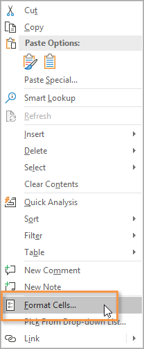
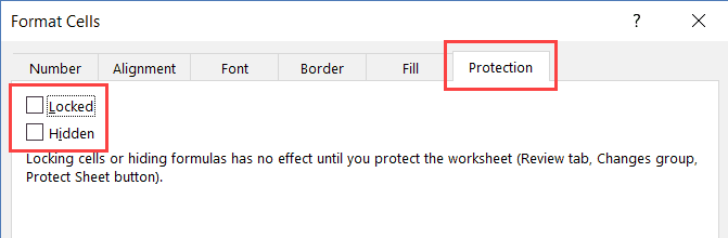
This will bring up the Format Cells window (keyboard shortcut for this window is Ctrl + 1.). Choose the tab that says Protection.
Next, make sure that the Locked option is checked.
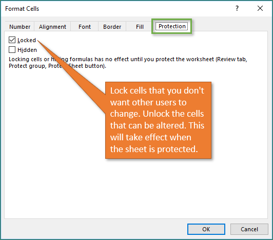
Locked is the default setting for all cells in a new worksheet/workbook.
Once we protect the worksheet (in the next step) those locked cells will not be able to be altered by users.
If you want users to be able to edit a particular cell or range, uncheck the Locked box so they are unlocked. Since cells are locked by default, most of the job will be going through the sheet and unlocking cells that can be edited by users.
I share some shortcuts to make this process faster in the Bonus section below.
Step 2: Protect the Worksheet
Now that you’ve locked/unlocked the cells that you want users to be able to edit, you want to protect the sheet. Once you protect the sheet, users cannot change the locked cells. However, they can still modify the unlocked cells.
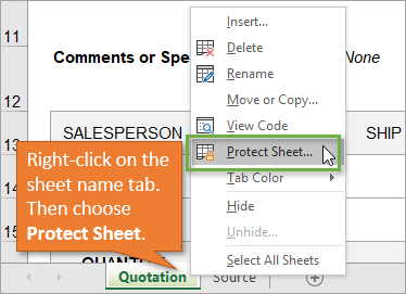
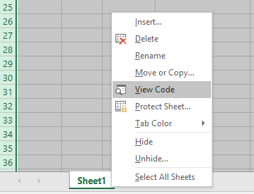
To protect the sheet, simply right-click on the tab at the bottom of the sheet, and choose Protect Sheet… from the menu.
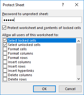
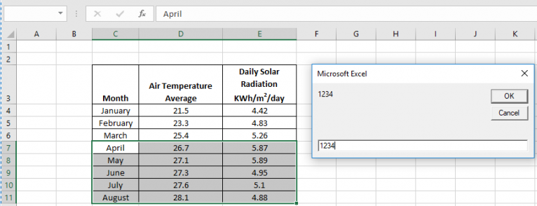
This will bring up the Protect Sheet window. If you want your sheet to be password protected, you have the option of entering a password here. Adding a password is optional. Click OK.
If you’ve chosen to enter a password, then you will be prompted to verify your entry after you’ve clicked OK.
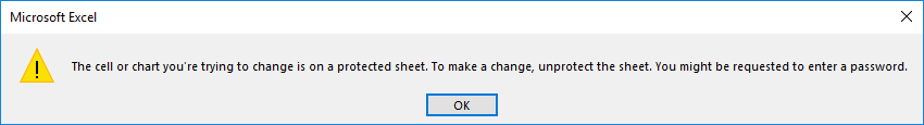
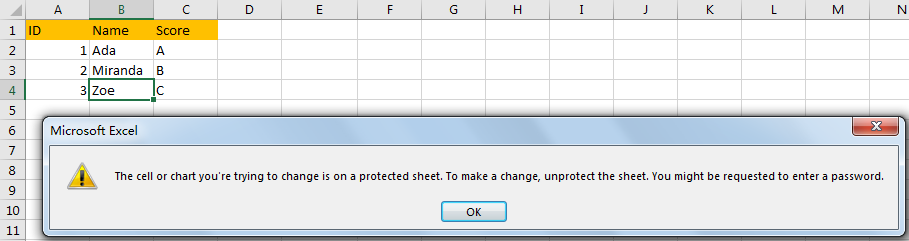
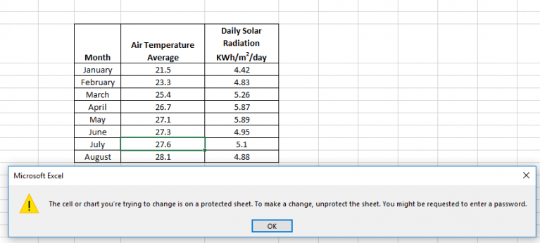
With the sheet protected, users will be unable to change the cells that are locked. If they try to make changes, they will get an error/warning message that looks like this.
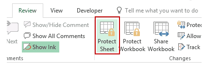
You can unprotect the sheet in the same way that you protected it, by right-clicking on the sheet tab. An alternative way to protect and unprotect sheets is by using the Protect Sheet button in the Review tab of the Ribbon.
The button text displays the opposite of the current state. It says Protect Sheet when the sheet is unprotected, and Unprotect Sheet when it is protected.
It’s important to note that all cells can be edited when the sheet is unprotected. After making changes you must protect the sheet again and Save the workbook before sending or sharing with other users.
3 Bonus Tips for Locking Cells and Protecting Sheets
As you can see, it is fairly simple to protect your formulas and formatting from being changed! But I’d like to leave you with three tips to help make it faster & easier for both you and your users.
1. Prevent Locked Cells From Being Selected
This tip will help make it faster and easier for your users to input data in the sheet.
Turning off the Select locked cells option prevents the locked cells from being selected with either the mouse or keyboard (arrow or tab keys). This means users will only be able to select the unlocked cells that they need to edit. They can quickly hit the Tab, Enter, or arrow keys to move to the next editable cell.
To make this change, you just uncheck the option that says “Select locked cells” on the Protect Sheet window.
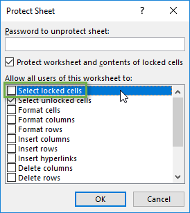
After pressing OK, you will only be able to select the unlocked cells.
2. Add a button for locking cells to the Quick Access Toolbar
This allows you to quickly see the locked setting for a cell or range.
From the Home tab on the Ribbon, you can open the drop-down menu under the Format button and see the option to Lock Cell.
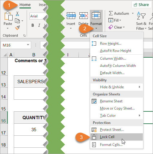
If you right-click on the Lock Cell option, another menu appears giving you the option to add the button to the Quick Access Toolbar.
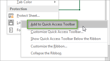
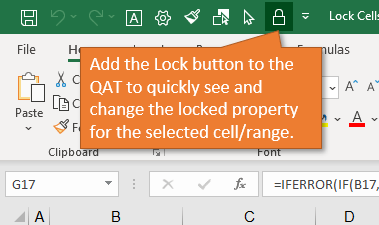
When you select this option, the button will be added to the Quick Access Toolbar at the top of the workbook. This button will remain each time you use Excel. You can easily lock and unlock specific cells on your sheet by clicking on this button.
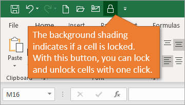
You can also see if the active cell locked or unlocked. The button will have a dark background if the selection is locked.
It’s important to note that this only shows the locked state of the active cell. If you have multiple cells selected, the active cell is the cell you selected first and appears with no fill shading.
Mixed Lock State
If you select a range that contains both locked and unlocked cells, you will see a solid box for the Locked checkbox in the Format Cells window. This denotes the mixed state.
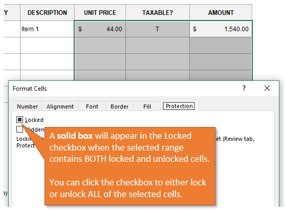
You can click the checkbox to lock or unlock ALL cells in the selected range.
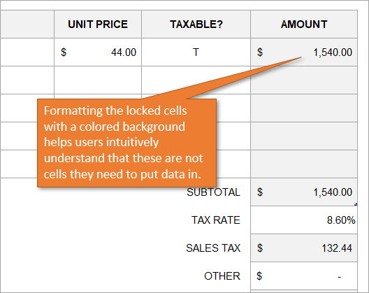
3. Use different formatting for locked cells
By changing the formatting of cells that are locked, you give your users a visual clue that those cells are off limits. In this example the locked cells have a gray fill color. The unlocked (editable) cells are white. You can also provide a guide on the sheet or instructions tab.
You might be wondering where I found this template for a quote. I got it from the template library. You can access the library by going to the File tab, choosing New, and using the search word “quote.”
You can find all sorts of useful templates there, including invoices, calendars, to-do lists, budgets, and more.
Conclusion
By locking your cells and protecting your sheet, you can keep your formulas safe from tampering by other users, and prevent mistakes.
I hope this simple tutorial proves helpful to you. Please leave a comment below if you have any tips or questions about locking cells, protecting sheets with passwords, or preventing users from changing cells.
Thank you! 🙂
Data in Excel can be protected from extraneous interference. This is important, because sometimes you spend a lot of time and effort creating a pivot table or a large array, and another person accidentally or intentionally changes or completely deletes all your work.
Let’s consider the ways of protecting an Excel document and its single elements.
Protection of Excel cells from changing
How to put protection on a cell in Excel? By default, all cells in Excel are protected (locked). It’s easy to check: right-click on any cell, select «Format Cells» – «Protection». We can see that the check box on the «Locked» item is selected. But this does not mean that they are protected from changes.
Why do we need this information? The thing is that Excel doesn’t provide the function allowing you to protect a single cell. We can enable protection of the worksheet, and then all the cells on it will be protected from editing and other interference. On the one hand, it is convenient, but what if we don’t need to protect all the cells, but only some of them?
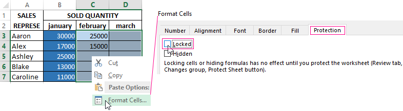
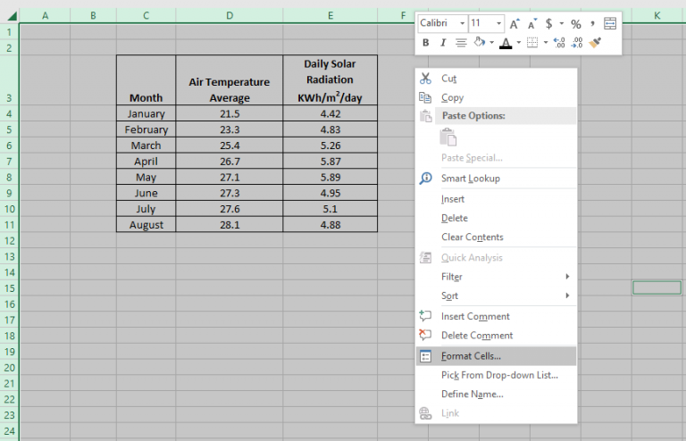
Let’s consider an example. We have a simple spreadsheet with data. We need to send this spreadsheet to branch stores, so that the stores could fill in the «SOLD QUANTITY» column and send it back. To avoid making any changes to other cells, let’s protect them.
First, remove protection from those cells to which employees of branch stores will make changes. Select C3: D7, right-click to open the menu, select «Format Cells» and remove the check box from «Locked».
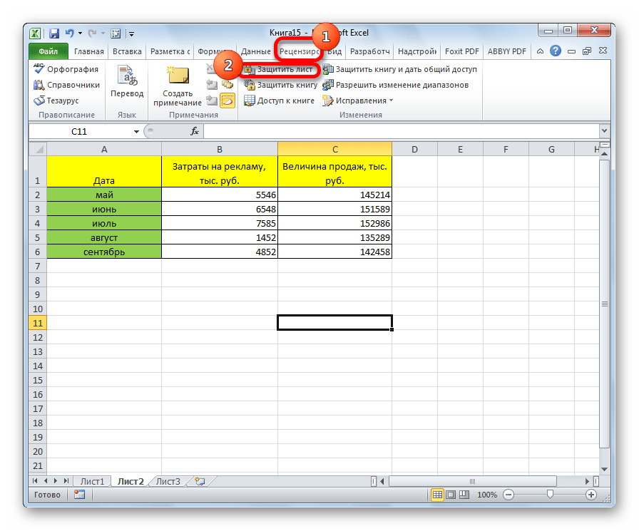
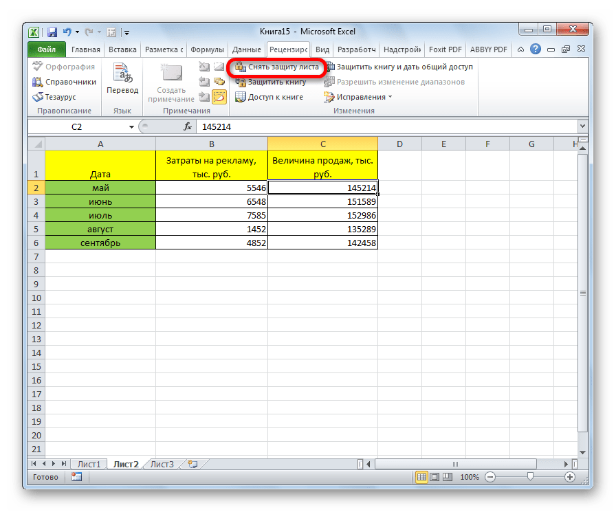
Now select «REVIEW» – «Changes» — «Protect Sheet» tab. A window appears with 2 check boxes selected. Clear the first one, to exclude any interference of branch stores’ employees, except for filling «SOLD QUANTITY» column. Come up with a password and click OK.
Warning! Do not forget your password!
Now other people can only enter some value in C3: D7 range. Since we have limited all other actions, no one can even change the background color. All the formatting tools on the top toolbar aren’t active, that is, they do not work.
Protection of an Excel workbook from editing
If several people work on one computer, it is advisable to protect their documents from editing by third parties. It is possible to put protection not only on separate worksheets, but also on the whole workbook.
When the workbook is protected, outsiders can open the document, see the written data, but they cannot rename the sheets, insert a new one, change their location, etc. Let’s have a try.
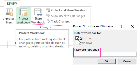
Save the previous formatting. That is, you still can make changes only in «SOLD QUANTITY» column. To protect the workbook completely, select «REVIEW» – «Changes» — «Protect Workbook» tab. Click the check box opposite «Structure» item and come up with a password.
Now, if we try to rename the worksheet, we will not succeed. All commands are gray-colored: they don’t work.
The protection from the worksheet and the workbook is removed with the same buttons. When removing, the system will require the same password.
Содержание
- Включение блокирования ячеек
- Способ 1: включение блокировки через вкладку «Файл»
- Способ 2: включение блокировки через вкладку «Рецензирование»
- Разблокировка диапазона
- Вопросы и ответы

При работе с таблицами Excel иногда возникает потребность запретить редактирование ячейки. Особенно это актуально для диапазонов, где содержатся формулы, или на которые ссылаются другие ячейки. Ведь внесенные в них некорректные изменения могут разрушить всю структуру расчетов. Производить защиту данных в особенно ценных таблицах на компьютере, к которому имеет доступ и другие лица кроме вас, просто необходимо. Необдуманные действия постороннего пользователя могут разрушить все плоды вашей работы, если некоторые данные не будут хорошо защищены. Давайте взглянем, как именно это можно сделать.
Включение блокирования ячеек
В Экселе не существует специального инструмента, предназначенного для блокировки отдельных ячеек, но данную процедуру можно осуществить с помощью защиты всего листа.
Способ 1: включение блокировки через вкладку «Файл»
Для того, чтобы защитить ячейку или диапазон нужно произвести действия, которые описаны ниже.
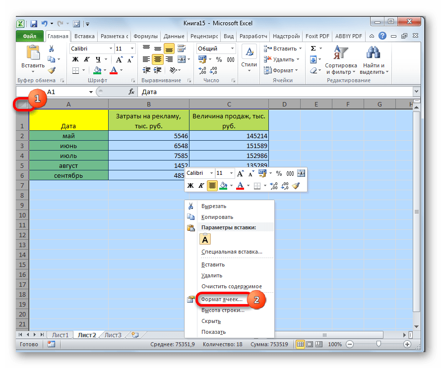
- Выделите весь лист, кликнув по прямоугольнику, который находится на пересечении панелей координат Excel. Кликните правой кнопкой мыши. В появившемся контекстном меню перейдите по пункту «Формат ячеек…».
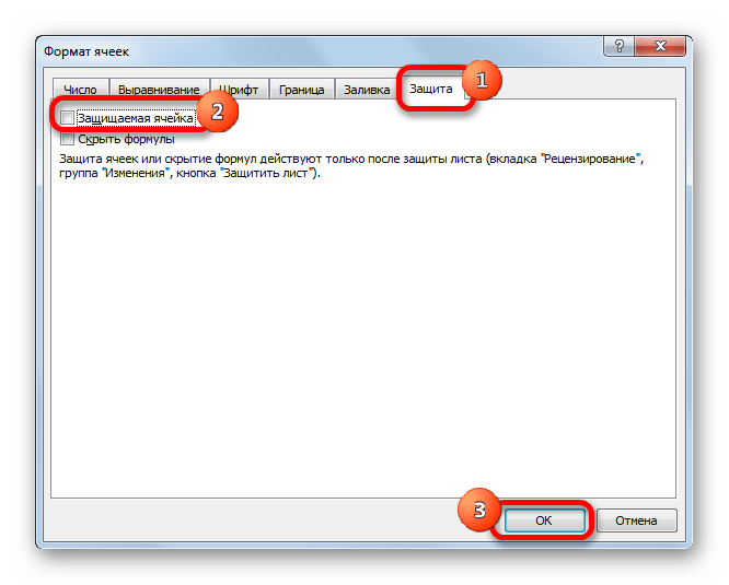
- Откроется окно изменения формата ячеек. Перейдите во вкладку «Защита». Снимите галочку около параметра «Защищаемая ячейка». Нажмите на кнопку «OK».
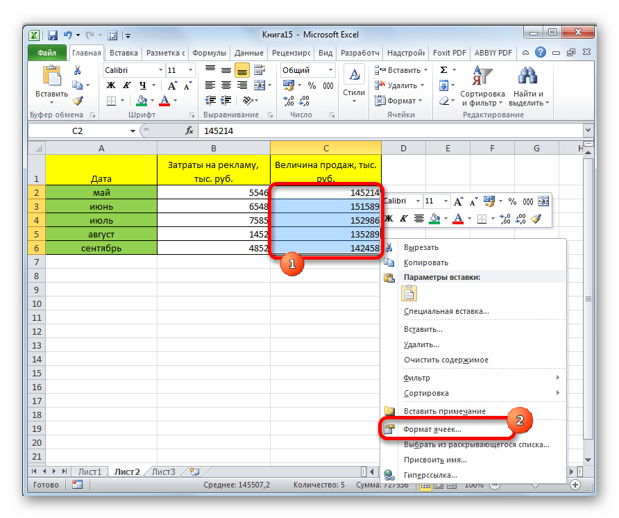
- Выделите диапазон, который желаете заблокировать. Опять перейдите в окно «Формат ячеек…».
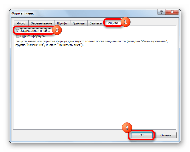
- Во вкладке «Защита» поставьте галочку у пункта «Защищаемая ячейка». Кликните по кнопке «OK».

Но, дело в том, что после этого диапазон ещё не стал защищенным. Он станет таковым только тогда, когда мы включим защиту листа. Но при этом, изменять нельзя будет только те ячейки, где мы установили галочки в соответствующем пункте, а те, в которых галочки были сняты, останутся редактируемыми.
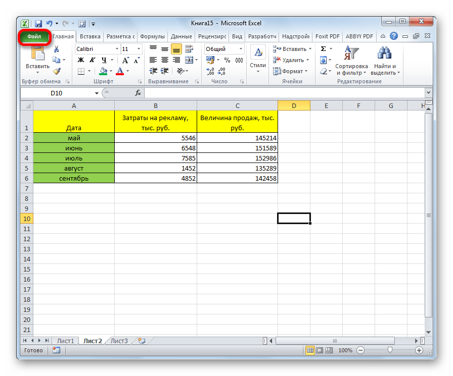
- Переходим во вкладку «Файл».
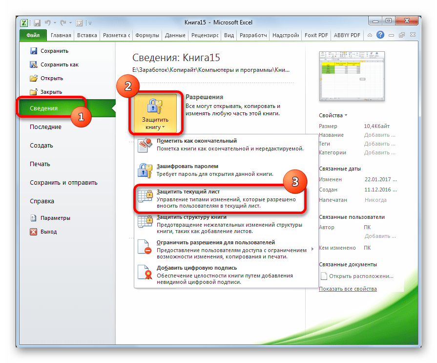
- В разделе «Сведения» кликаем по кнопке «Защитить книгу». В появившемся списке выбираем пункт «Защитить текущий лист».
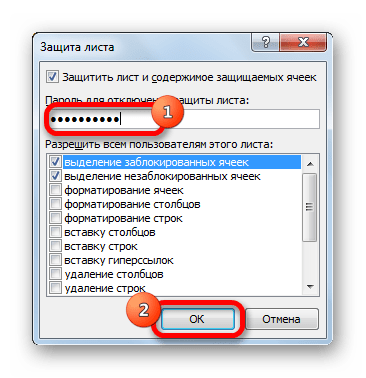
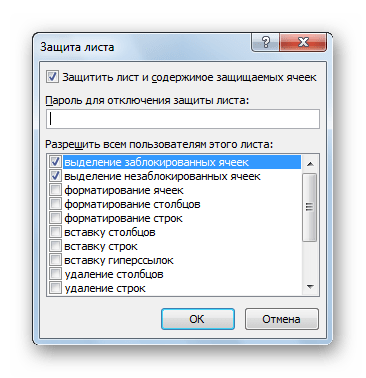
- Открываются настройки защиты листа. Обязательно должна стоять галочка около параметра «Защитить лист и содержимое защищаемых ячеек». При желании можно установить блокирование определенных действий, изменяя настройки в параметрах, находящихся ниже. Но, в большинстве случаев, настройки выставленные по умолчанию, удовлетворяют потребностям пользователей по блокировке диапазонов. В поле «Пароль для отключения защиты листа» нужно ввести любое ключевое слово, которое будет использоваться для доступа к возможностям редактирования. После того, как настройки выполнены, жмем на кнопку «OK».
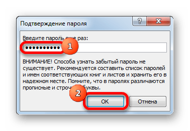
- Открывается ещё одно окно, в котором следует повторить пароль. Это сделано для того, чтобы, если пользователь в первый раз ввел ошибочный пароль, тем самым навсегда не заблокировал бы сам себе доступ к редактированию. После ввода ключа нужно нажать кнопку «OK». Если пароли совпадут, то блокировка будет завершена. Если они не совпадут, то придется производить повторный ввод.
Теперь те диапазоны, которые мы ранее выделили и в настройках форматирования установили их защиту, будут недоступны для редактирования. В остальных областях можно производить любые действия и сохранять результаты.
Способ 2: включение блокировки через вкладку «Рецензирование»
Существует ещё один способ заблокировать диапазон от нежелательного изменения. Впрочем, этот вариант отличается от предыдущего способа только тем, что выполняется через другую вкладку.
- Снимаем и устанавливаем флажки около параметра «Защищаемая ячейка» в окне формата соответствующих диапазонов точно так же, как мы это делали в предыдущем способе.
- Переходим во вкладку «Рецензирование». Кликаем по кнопке «Защитить лист». Эта кнопка расположена в блоке инструментов «Изменения».
- После этого открывается точно такое же окно настроек защиты листа, как и в первом варианте. Все дальнейшие действия полностью аналогичные.

Урок: Как поставить пароль на файл Excel
Разблокировка диапазона
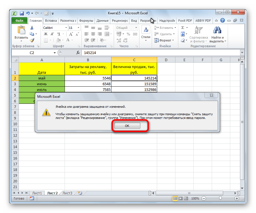
При нажатии на любую область заблокированного диапазона или при попытке изменить её содержимое будет появляться сообщение, в котором говорится о том, что ячейка защищена от изменений. Если вы знаете пароль и осознано хотите отредактировать данные, то для снятия блокировки вам нужно будет проделать некоторые действия.
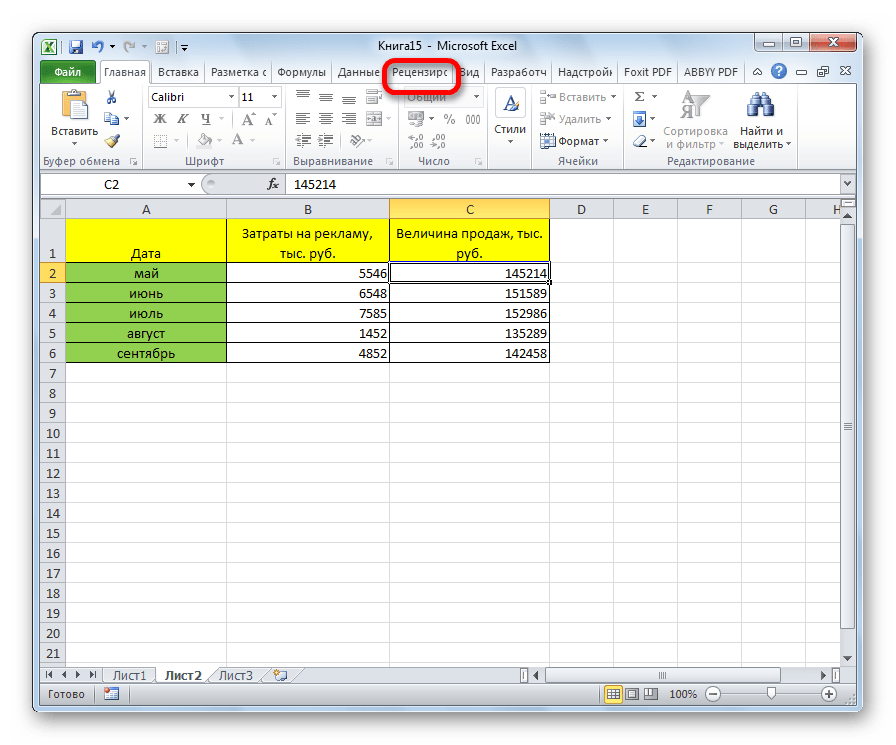
- Переходим во вкладку «Рецензирование».
- На ленте в группе инструментов «Изменения» кликаем по кнопке «Снять защиту с листа».
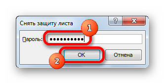
- Появляется окошко, в которое следует ввести ранее установленный пароль. После ввода нужно кликнуть по кнопке «OK».
После этих действий защита со всех ячеек будет снята.
Как видим, несмотря на то, что в программе Эксель не имеется интуитивно понятного инструмента для защиты конкретной ячейки, а не всего листа или книги, данную процедуру можно выполнить путем некоторых дополнительных манипуляций через изменение форматирования.
Еще статьи по данной теме:
Помогла ли Вам статья?
When it comes time to send your Excel spreadsheet, it’s important to protect the data that you’re sharing. You might want to share your data, but that doesn’t mean it should be changed by someone else.
Spreadsheets often contain essential data that shouldn’t be modified or removed by the recipient. Luckily, Excel has built-in features to protect your spreadsheets.
In this tutorial, I’ll help you make sure that your Excel workbooks maintain data integrity. Here are three key techniques you’ll learn in this tutorial:
- Password protect entire workbooks to prevent them from being opened by unauthorized users.
- Protect individual sheets and the workbook structure, to prevent the insertion or deletion of sheets in the workbook.
- Protect cells, to specifically allow or disallow changes to key cells or formulas in your Excel spreadsheets.
Even users with the best intentions may accidentally break an important or complex formula. The best thing to do is remove the option to change your spreadsheets altogether.
How to Protect Excel: Cells, Sheets, & Workbooks (Watch & Learn)
In the screencast below, you’ll see me work through several important types of protection in Excel. We’ll protect an entire workbook, a single spreadsheet, and more.
Want a step-by-step walkthrough? Check out my steps below to find out how to use these techniques. You’ll learn how to protect your workbook in Excel, as well as protecting individual worksheets, cells, and how to work with advanced settings.
We start with broader worksheet protections, then work down to narrower targeted protections you can apply in Excel. Let’s get started learning how to protect your spreadsheet data:
1. Password Protect an Excel Workbook File
Let’s start off by protecting an entire Excel file (or workbook) with a password to prevent others from opening it.
This is a breeze to do. While working in Excel, navigate to the File tab choose the Info tab. Click on the Protect Workbook dropdown option and choose Encrypt with Password.
As is the case with any password, choose a strong and secure combination of letters, numbers, and characters, bearing in mind that passwords are case-sensitive.


It’s important to note that Microsoft has really beefed up the seriousness of their password protection in Excel. In prior versions, there were easy workarounds to bypass password protection of Excel workbooks, but not in newer versions.


In Excel 2013 and beyond, the password implementation will prevent these traditional methods to bypass it. Make sure that you store your passwords carefully and safely or you risk permanently losing access to your crucial workbooks.
Excel Workbook — Mark as Final
If you want to be a bit less forceful with your spreadsheets, consider using the Mark as Final feature. When you mark an Excel file as the final version, it switches the file to read-only mode, and the user will have to re-enable editing.
To change a file to read-only mode, return to the File > Info button, and click on Protect Workbook again. Click on Mark as Final and confirm that you want to mark the document as a final version.


Marking a file as the final version will add a soft warning to the top of the file. Anyone who opens the file after it has been marked as final will see a notice, warning them that the file is finalized.


Marking a file as the final version is a less formal way of signaling that a file shouldn’t be changed further. The recipient still has the ability to click Edit Anyway and modify the spreadsheet. Marking a file as the final edition is more like a suggestion, but it’s a great approach if you trust the other file users.
2. Password Protect Your Excel Sheet Structure
Next up, let’s learn how to protect the structure of an Excel workbook. This option will ensure that no sheets are deleted, added, or re-arranged inside of the workbook.
If you want everyone to be able to access the workbook, but limit the changes they can make to a file, this is a great start. This protects the structure of the workbook, and limits how the user can change the sheets inside of it.
To turn on this protection, go to the Review tab on Excel’s ribbon and click on Protect Workbook.


Once this option is turned on, the following will go into effect:
- No new sheets can be added to the workbook.
- No sheets can be deleted from the workbook.
- Sheets can no longer be hidden or unhidden from the user’s view.
- The user can no longer drag and drop the sheet tabs to reorder them in the workbook.
Of course, trusted users can be given the password to unprotect the workbook and modify it. To unprotect a workbook, simply click on the Protect Workbook button again and input the password to unprotect the Excel workbook.


3. How to Protect Cells in Excel
Now, let’s get down to really detailed methods for protecting a spreadsheet. So far, we’ve been password protecting an entire workbook or the structure of an Excel file. In this section, we dig into how to protect your cells in Excel with specific settings you can apply. We cover how to allow or block certain types of changes to be made to parts of your spreadsheet.
To get started, find Excel’s Review tab, and click on Protect Sheet. On the pop-up window, you’ll see a huge set of options. This window allows you to fine-tune how you want to protect the cells in your Excel spreadsheet. For now, let’s leave the settings at their default.


This option allows for very specific protections of your spreadsheet. By default, the options will almost totally lock down the spreadsheet. Let’s add a password so that the sheet is protected. If you press OK at this point, let’s see what happens when you attempt to change a cell.


Excel throws off an error that the cell is protected, which is exactly what we wanted.
Basically, this option is crucial if you want to ensure that your spreadsheet isn’t changed by others who have access to the file. Using the protect sheet feature is a way that you can selectively protect the spreadsheet.
To unprotect the sheet, simply click on the Protect Sheet button and re-enter the password to remove the protections added to the sheet.
Specific Protections in Excel
Let’s take a second look at the options that show when you start to protect a sheet in Excel workbooks.

The Protect Sheet menu lets you refine the options for sheet protection. Each of the boxes on this menu lets the user change slightly more inside of a protected worksheet.
To remove a protection, check the respective box in the list. For example, you could allow the spreadsheet user to Format cells by checking the corresponding box.
Here are two ideas on how you could selectively allow the user to change the spreadsheet:
- Check the Format cells, columns, and rows boxes to let the user change the visual appearance of cells without modifying the original data.
- Insert columns and rows could be checked so that the user can add more data, while protecting the original cells.
The important box to leave checked is the Protect worksheet and contents of locked cells box. This protects the data inside of cells.
When you’re working with crucial financial data or formulas that will be used in making decisions, you have to maintain control of the data and ensure that it doesn’t change. Using these types of targeted protections is an important Excel skill to master.
Recap and Keep Learning More About Excel
Locking up a spreadsheet before you send it is crucial to protecting your valuable data and making sure that it’s not misused. The tips I shared in this tutorial help you maintain control of that data even after your Excel spreadsheet is forwarded and shared.
All of these tips are additional tools and steps to becoming an advanced Excel user. Protecting your workbooks is a specific skill, but there are lots of ways to improve your performance. As always, there’s room to grow your Excel skills further. Here are some helpful Excel tutorials with important skills to master next:
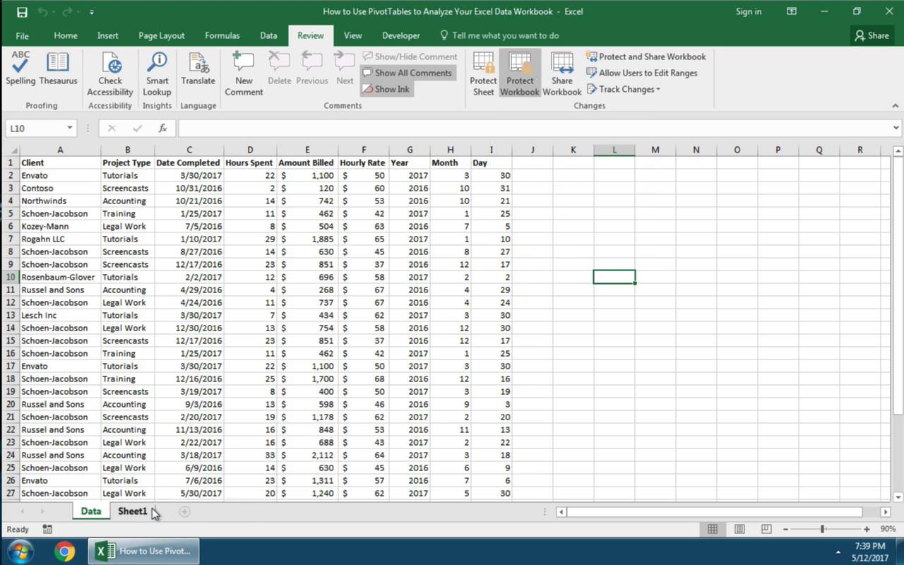
- PivotTables are a great tool for working with spreadsheet data. Here’s 5 Advanced Excel Pivot Table Techniques to learn now.
- ExcelZoo has a listing of additional tutorials for protecting your workbooks, sheets, and cells.
- Condition formatting changes how a cell looks based on what’s inside of it. Here’s a comprehensive Excel tutorial on How to Use Conditional Formatting.
How do you protect your important business data when sharing it? Let me know in the comments section if you use these protection tools or others I may not know about.
Did you find this post useful?

I believe that life is too short to do just one thing. In college, I studied Accounting and Finance but continue to scratch my creative itch with my work for Envato Tuts+ and other clients. By day, I enjoy my career in corporate finance, using data and analysis to make decisions.
I cover a variety of topics for Tuts+, including photo editing software like Adobe Lightroom, PowerPoint, Keynote, and more. What I enjoy most is teaching people to use software to solve everyday problems, excel in their career, and complete work efficiently. Feel free to reach out to me on my website.
Many users used to lock cells in Excel so that no one can modify the content of the protected cells without their permission. Thus, if you also want to restrict someone from making changes to your Excel cells then read this blog. This post contains different ways to lock Excel cells and make them protected.
Quick Ways |
Step-By-Step Solutions Guide |
|
Way 1- Lock Cells In Excel Worksheet |
Choose the cells >> go to the Home tab and then from the Alignment…Complete Steps |
|
Way 2- Lock Some Specific Cells In Excel |
Choose the entire worksheet >> go to Home tab >> hit sign of the dialog box launcher…Complete Steps |
|
Way 3- Lock Excel Cells Using VBA Code |
Choose entire cells in Excel spreadsheet >> go to the Home tab >> cells >> Format…Complete Steps |
|
Way 4- Protect Entire Worksheet Except Few Cells |
Press Control + 1 key >> in the opened Format Cells dialog box >> go to ‘Protection’...Complete Steps |
|
Way 5- Lock Formula Cells |
Choose Format Cells >> go to Protection tab >> untick Locked option >> OK…Complete Steps |
To repair & recover corrupted Excel file data, we recommend this tool:
This software will prevent Excel workbook data such as BI data, financial reports & other analytical information from corruption and data loss. With this software you can rebuild corrupt Excel files and restore every single visual representation & dataset to its original, intact state in 3 easy steps:
- Download Excel File Repair Tool rated Excellent by Softpedia, Softonic & CNET.
- Select the corrupt Excel file (XLS, XLSX) & click Repair to initiate the repair process.
- Preview the repaired files and click Save File to save the files at desired location.
What’s The Need To Lock Cells In Excel?
The plus point of locking cells in Excel is that it protects your data from the unwanted changes.
Suppose you have to share your Excel spreadsheet with other users and there are some specific cells which you don’t want to get modified. In that case, cell lock is the best trick to avoid formula and formatting changes like issues.
Way 1- Lock Cells In Excel Worksheet
Follow the below-mentioned solutions to do so:
- Choose the cells which you need to lock.
- Go to the Home tab and then from the Alignment group tap to the small arrow present across it. This will open the windows of Format Cells.
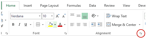
- Now in the format cell window go to the Protection tab and choose the check box of Locked After that tap to the OK button to shut off this popup window.

Note: If you are attempting these steps on the worksheet or workbook which you haven’t protected then you will find that the cells are locked already. This implies that the cell can also be locked when the workbook or worksheet is protected.
- From the excel ribbon hit the Review After that from the Changes group, you have to choose either the Protect Workbook or Protect Sheet.
- Next, you have to reapply the protection over your workbook or worksheet.
Tip: well it’s a best solution to unlock cells which you need to modify before protecting a workbook or worksheet. But don’t get worried as you can unlock them easily even after applying protection over it. For removing up the protection, all you need to do is just remove the applied password.
Also Read: 5 Tricks To Protect Excel Workbook From Editing
Way 2- Lock Some Specific Cells In Excel
Sometimes you just need to lock some individual cells which contain important data or formulas. In such cases, only protect the cells which you need to lock leaving the rest one as it is.
By default, entire cells are comes locked, so if you apply protection to your sheet then entire cells are also get locked.
So, make sure that only those cells are protected which you want to lock and after that only apply protection to the whole worksheet.
Follow the steps to lock some specific cells in Excel
- Choose entire worksheet and then go to the Home tab.
- After that hit, the sign of the dialog box launcher presents the alignment group.
- Now in the opened dialog box of Format Cells, got to the Protection tab and uncheck the Locked option. Hit the OK button.
- Choose the cells which you need to lock.
- Again make a tap over the dialog box launcher present in the Alignment group which is under the Home tab.
- Now again in the opened dialog box of Format Cells go to the Protection tab and make a check mark across the Locked option.
- Doing this will unlock entire cells of your worksheet except the one which you have selected for locking.
- Now go to the Review tab and then from the Changes group hit the Protect Sheet option.
- From the opened dialogue box of Protect Sheet:
- Check whether the option of ‘Protect worksheet and contents of locked cells’ is checked or not. If it’s not then check it.

- Enter the password to apply password on your sheet.

- Now specify the permission which you want to assign to other users. By default, you will see that the first two options are already selected. Using which user can easily make selection for the locked or unlocked cells.
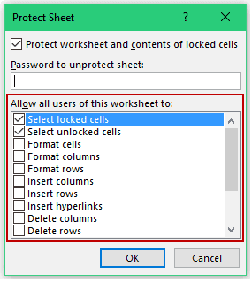
- Apart from this you can also allow other options like inserting rows/columns or making changes in the formatting.
- Tap to the OK button.

If you are applying any password then you are asked to reconfirm it.
When the next time you try to edit those specific cells, you will get the following error message pop-up dialog box.
Way 3- Lock Excel Cells Using VBA Code
- Choose entire cells in your Excel spreadsheet.
- Now go to the Home tab first and then to cells from this cell section tap on the Format option and choose the format cells option.
- This will open a Format Cells dialogue box. On this opened dialog box, you need hit the Protection tab. Here you have un-select the option Locked.

- Now in your Excel file where name of your sheet appears. Make a right click from your mouse and choose the View Code.
- This will open Microsoft Visual Basic for Applications dialogue box. In this opened white sheet along with the dialogue box, you just need to type the below code.
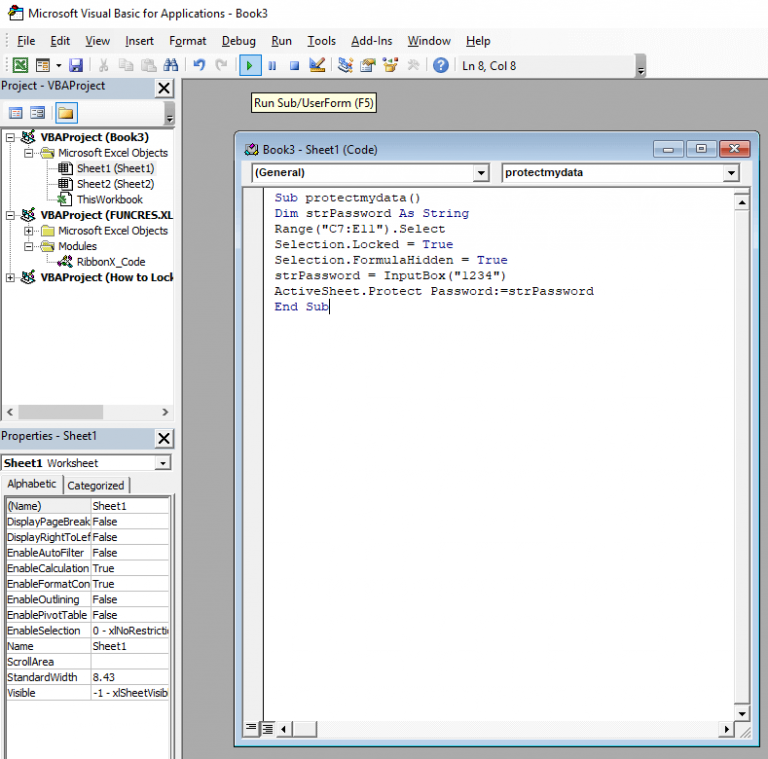
- In the written code, we have selected the data range from C7 to E11. And have also applied a password like, 1234.
- After entering the complete code go to the Debug Here you will find a Run Sub/User Form (F5) option tap on it.
- Now you will see that your Excel worksheet is opening along with a password window.
- So, write same password that you as allotted in the VBA code eg: 1234.
- After doing this whenever you approach for making changes in the desired cells of the Excel. This will throw a warning message stating that “you can’t edit the cells as it is protected”.
Note: To unlock the cells locked with Excel VBA code you have to follow the same unlocking procedures as explained earlier.
Also Read; Top 3 Methods To Unlock Password Protected Excel File
Way 4- Protect Entire Worksheet Except Few Cells
In some cases, people also want to protect the entire worksheet by keeping some of the cells unlocked.
Well, such a situation arises when you have added interactive features in your worksheet like a drop-down list. And you want that your drop-down keeps working even when the worksheet is protected.
To accomplish this task, just follow the below-mentioned steps:
- Make a selection of the cells which you want to keep unlocked.
- Press the Control + 1 key from your keyboard.
- In the opened Format Cells dialog box go to the ‘Protection’.
- Unselect the Locked option and hit the OK button.
Now if the entire worksheet is kept protected, these particular cells should work normally.
For this you have to perform the following steps, so as to protect the entire worksheet except the selected cells:
- Hit the Review tab and then from the Changes group tap to the Protect Sheet icon.
- In the opened Protect Sheet dialog box:
- Check whether the option of ‘Protect worksheet and contents of locked cells’ is checked or not. If it’s not then check it.

- Enter the password to apply password on your sheet).
- Now specify the permission which you want to assign to other users. By default, you will see that the first two options are already selected. Using which user can easily make selection for the locked or unlocked cells.
- Apart from this you can also allow other options like inserting rows/columns or making changes in the formatting.

Way 5- Lock Formula Cells
To lock formula cells, the very first thing you need to do is unlock all the cells and then only lock the cells having the formula in it. At last protect the sheet.
Well if you don’t know how to perform all these tasks then follow the below steps:
- Choose entire cell of your worksheet.

- Now make a right click and from the listed option choose the Format Cells.
- On the opened format cell window go to the Protection tab and untick the check box of Locked option. After that hit the OK button.

- Go to the Home tab and then from the Editing group choose the Find & Select.

- Hit the Go To Special option.

- Choose Formulas and hit the OK button.
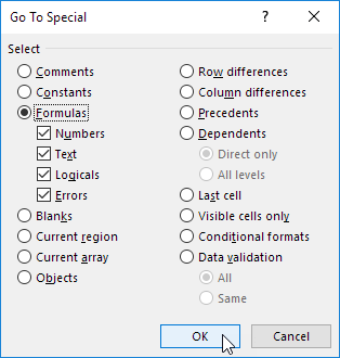
You will see that after doing these steps Excel will selects all the formula cells.

- Press the CTRL + 1 button from your keyboard.
- Go to the Protection tab and select the check box of Locked option. After that press the OK button.
Note:
If you select the check box of Hidden option then the user will not be able to see the formula within the formula bar even after choosing the formula cells.
Always keep in mind that locking cells doesn’t have any effect until and unless the worksheet is protected.
- So now it’s time to protect your Excel sheet.
After this, you will see that entire the formula cells are been locked. In case of editing these cells, firstly you need to unprotect the worksheet.
Use Excel Repair Tool to Repair/Recover Corrupted Excel Documents
MS Excel Repair Tool is a special tool that is specifically designed to repair any sort of issues, corruption, errors in Excel file. This can also easily restore entire lost Excel data including cell comments, charts, worksheet properties, and other related data.
It is a unique tool that can repair multiple corrupted Excel files in one repair cycle and restore data to a new blank Excel file or the preferred location. The tool has the ability to recover data without modifying the original formatting.
- The interface is very simple, with a large toolbar of buttons to add files or folders to the application.
- With this software, you can repair your corrupted Excel file.
- It can easily restore all corrupt excel files and also recover everything which includes cell comments, charts, worksheet properties, and other related data.
- The corrupted excel file can be restored to a new blank Excel file.
- It has the ability to recover the complete Excel file data from the file and restore them even without modifying the original formatting.
* Free version of the product only previews recoverable data.
Steps to Utilize MS Excel Repair Tool:
Related FAQs:
Can I Lock Multiple Cells in Excel?
Yes, you can lock multiple cells in Excel through freeze panes. Apart from that, you can use a shortcut key- F4 to lock specific columns or rows in the document as well as the range of cells that you want to lock.
How Do I Make a Cell Non-Editable in Excel?
To make a cell non editable in Excel, you need to make cell as read only using VBA code. Although using the VBA code helps to make cell as read-only so that no one can edit them and even you don’t have to lock the cells to protect your worksheet data.
Does F4 Lock Cells in Excel?
Yes, the F4 key is a shortcut mode or we can say the easiest way to lock cells in the MS Excel.
Bottom Line
Locking cells in Excel help you to keep the formula completely safe from being tempered by any third-party user.
Hopefully, this informative tutorial seems helpful to you on how to protect cells in excel without protecting sheets. Don’t forget to leave a comment if you have any queries or tips to share about how to lock cells in Excel and protect them.


Priyanka is an entrepreneur & content marketing expert. She writes tech blogs and has expertise in MS Office, Excel, and other tech subjects. Her distinctive art of presenting tech information in the easy-to-understand language is very impressive. When not writing, she loves unplanned travels.
At times, the excel sheet we are working on has some important information. Cells containing functions and formulas are so crucial that losing them can create huge problems for us. However, protecting a cell in excel can solve these problems as it can define which cells can be used for data entry or editing. Securing excel cells using passwords is a secure and effective method.
In this guide, you will learn how to protect a cell in excel from unwanted use. Just prevent a cell and specific cells from editing, leaving other cells to be edited or changed. But if the cells locked by accident or forgot the password of how to unprotect it, here also gives a ultimate solution – PassWiper for Excel to help you out.
Part 1. How to Protect Cells in Excel without Protecting Sheet
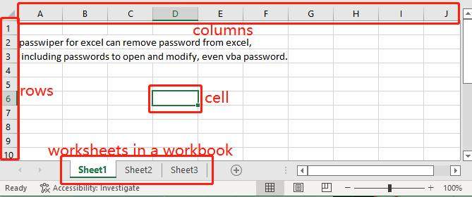
First let’s understand what is cell and row and column in excel. Cells can make up a row, rows can make up a column, columns makes up a sheet. Sheets to Workbook. This is the simple knowledge of excel. Here we will learn how to protect a cell and cell ranges (specific cells) in excel, ’cause protecting all cells means lock excel worksheet, this step you can click ‘Info’ to lock it.
Now we have known which part of excel we need to protect. You can protect a single cell and cell ranges in Excel in several ways that will only allow others to read, but not edit your protected data. This guide will help you to learn how to protect a cell from editing in excel.
Here are 3 easy ways to protect cells in Excel.
- 1. Protecting a Single Cell in Excel
- 2. Protecting Cell Ranges in Excel
- 3. Protecting Formula Cells
Way 1. Protecting a Cell in Excel
You can protect a specific cell in excel by following the below-mentioned steps.
Note: Pay attention to these steps as the steps involved in this way are used in other ways as well.
Step 1. Before protecting a cell, you need to unprotect all of the cells on your sheet. You can do this by selecting all of the cells in your worksheet. Right-click, and from the menu, select the ‘Format Cells’ option.
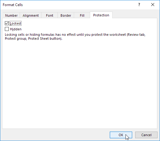
Step 2. This will open the Format Cells window. From there, select the Protection tab. Uncheck the ‘Locked’ checkbox then click OK.

Step 3. Now, select the cell that you want to protect. Right-click again, and select the ‘Format Cells’ option.
Step 4. Select the Protection tab from the Format Cells window. This time check the ‘Locked’ checkbox and click OK.
Step 5. The protection of a cell will only take effect when you protect the worksheet as well. For this purpose, go to the Review tab from the toolbar and select the option ‘Protect Sheet’.

Step 6. You will see a Protect sheet window. You can enter a password to protect the sheet if you want. However, this is optional. Click OK.
Way 2. Protecting Cells Ranges in Excel
Excel also gives you the ability to protect cells in a spreadsheet. However, protecting cells in excel is not the same as protecting an Excel file. This way is specifically for protecting cells in excel.
Step 1. On the worksheet, select just the cells that you want to lock.
Step 2. Bring up the Format Cells popup window again (Ctrl+Shift+F). This time, on the Protection tab, check the Locked box and then click OK. On the Review tab, click Protect Sheet.
Step 3. In the Allow all users of this worksheet to list, choose the elements that you want users to be able to change.
Way 3. Protecting Formula Cells
Protecting formula cells is crucial when dealing with sensitive data and calculations.
You can protect formula cells in your worksheet in the following steps.
Step 1. Open the Home Tab. Click ‘Editing’. Select ‘Find Select’. Choose ‘Go To Special’ from the drop-down menu.
Step 2. Now, check the ‘Formulas’ section along with the types of formulas. Once done, click OK.
Step 3. Now, press CTRL + 1 with the formulas selected.
Step 4. Now follow steps 4, 5, and 6 of Way 1 to protect the formula cells in excel.
Note: There’s no quick formula or shortcut to lock cells in excel, but you can create a macro to achieve it, but this way is difficult if you don’t know how to make a vba code. So this blog can solve all your worries.
Part 2. How to Unprotect Cells in Excel with/without Password
In the first part of this guide, we’ve discussed the ways of protecting a cell and cells in excel. In this way, only you’ll be able to edit those cells with knowing password.
Unlocking protected cells in excel is as easy as locking them when you get the password on hand.
Here’s a step-by-step procedure of how you can do it.
Step 1. Select that specific cell that you want to change when the sheet is protected.
Step 2. Navigate to the Review tab. Go to the Changes group. Click Allow Users to Edit Ranges (only available in an unprotected sheet).
Step 3. A dialog window will open up. From there, click New to add a new range of your choice.
Step 4. In this dialog window, you need to do the following:
- Type a range name
- Select a cell
- Type a password
- Click OK
Step 5. A Confirm password window will appear where you have to re-type the password to confirm. When done, click OK.
Step 6. Now, click the Protect Sheet button to protect the sheet.
Step 7. In this window, you have to type the password to unprotect the sheet. Now, check the boxes next to the actions you want to allow, click OK.
Step 8. Now re-type the password and click OK to finish!
Then your excel cells can be edited freely without any restrictions.
From the above parts, you probably understand how to password protect a cell in excel and how to change it. In the above part, you can change a protected cell if you know the password. But what if you forget the password and still need to change the cell urgently?
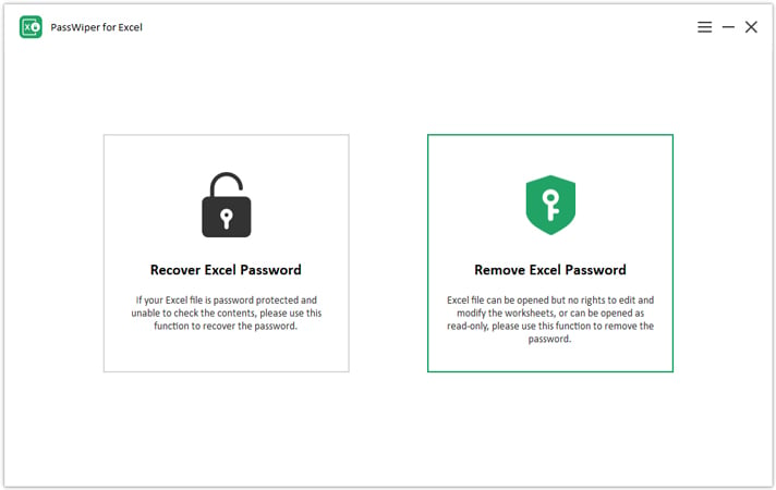
This is where PassWiper for Excel can help you out. It is an efficient and effective tool that can recover your excel passwords for you in just a few clicks. PassWiper for Excel can remove the restrictions in excel within easy three steps to unlock it. Regardless of the complexity and length of the password, you can easily unprotect the locked cells without password.
1. Download and install this tool in your computer.
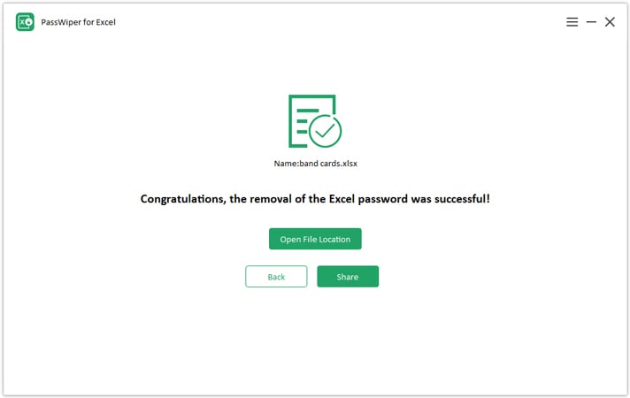
2. Select “Remove Excel Password”, then you can drag your excel file locked cells and then click “Remove”.
3. Then you can share the open excel file to your friends or co-workers and open it to edit the cells.
Summary
After reading through this guide, hope you’ve learned how to protect a cell in excel. You can protect the cells in several ways to prevent them from being used by untrusted users. Password-protected cells are secure. However, when you don’t know the password and want to make changes, don’t waste your precious time and try PassWiper for Excel as it is capable of recovering the excel password quickly. This tool has a higher recovery speed and causes no damage to your Excel data making it an ideal choice for excel password recovery.
![]()
Download Article
![]()
Download Article
Locking cells in an Excel spreadsheet can prevent any changes from being made to the data or formulas that reside in those particular cells. Cells that are locked and protected can be unlocked at any time by the user who initially locked the cells. Follow the steps below to learn how to lock and protect cells in Microsoft Excel versions 2010, 2007, and 2003.
To learn how to unlock the cells, read the article How to Open a Password Protected Excel File.
Things You Should Know
- In all versions of Excel, highlight and right click your cells. Then, select «Format Cells» > «Protection.» Check «Locked» and save.
- In Excel 2007 and 2010, go to «Review» > «Changes/Protect Sheet» > «Protect worksheet and contents of locked cells.» Type a password click through the prompts to save.
- In Excel 2003, go to «Tools» > «Protection» > «Protect Sheet.» Check «Protect worksheet and contents of locked cells.» Enter a password and follow the prompts to save.
-
1
Open the Excel spreadsheet that contains the cells you want locked.
-
2
Select the cell or cells you want locked.
Advertisement
-
3
Right-click on the cells, and select «Format Cells.»
-
4
Click on the tab labeled «Protection.»
-
5
Place a checkmark in the box next to the option labeled «Locked.»
-
6
Click «OK.»
-
7
Click on the tab labeled «Review» at the top of your Excel spreadsheet.
-
8
Click on the button labeled «Protect Sheet» from within the «Changes» group.
-
9
Place a checkmark next to «Protect worksheet and contents of locked cells.»
-
10
Enter a password in the text box labeled «Password to unprotect sheet.»
-
11
Click on «OK.»
-
12
Retype your password into the text box labeled «Reenter password to proceed.»
-
13
Click «OK.» The cells you selected will now be locked and protected, and can only be unlocked by selecting the cells once again, and entering the password you selected.


Advertisement
-
1
Open the Excel document that contains the cell or cells you want to lock.
-
2
Select one or all of the cells you want locked.
-
3
Right-click on your cell selections, and select «Format Cells» from the drop-down menu.
-
4
Click on the «Protection» tab.
-
5
Place a checkmark next to the field labeled «Locked.»
-
6
Click the «OK» button.
-
7
Click on the «Tools» menu at the top of your Excel document.
-
8
Select «Protection» from the list of options.
-
9
Click on «Protect Sheet.»
-
10
Place a checkmark next to the option labeled «Protect worksheet and contents of locked cells.»
-
11
Type a password at the prompt for «Password to unprotect sheet,» then click «OK.»
-
12
Reenter your password at the prompt for «Reenter password to proceed.»
-
13
Select «OK.» All the cells you selected will now be locked and protected, and can only be unlocked going forward by selecting the locked cells, and entering the password you initially set up.


Advertisement
Add New Question
-
Question
How do I lock cells in Excel without the whole document becoming read only?

I suppose you want to lock certain cells instead of the whole sheets. To do that, choose the whole sheet, right click and then select «Format Cells», then «Protection», then uncheck the «Locked» option and click okay. Then select the cells you want to lock, right click and select «Format Cells», then Protection; this time, check the «Locked» option and click okay. Now go back to the main tab, select «Review», then click on «Protect Sheet», and do whatever you want to do with it. Now only the cells you «locked» are protected from editing instead of the whole sheet.
-
Question
How can I protract the single cell while using Excel?
You cannot protract a single cell in Excel. You can, however, make it appear longer than the rest of the cells around it by «merging» two or more cells together. Highlight the cells you desire and right click. A menu will pop up allowing you to merge them.
-
Question
How do I allow changes to some cells of a protected sheet?
Select the whole worksheet by clicking the Select All button. On the Home tab, in the Font group, click the Format Cell Font dialog box launcher. On the Protection tab, clear the Locked box and then click OK.
Ask a Question
200 characters left
Include your email address to get a message when this question is answered.
Submit
Advertisement
Video
-
If multiple users have access to your Excel document, lock all cells that contain important data or complex formulas to prevent the cells from being accidentally changed.
-
If the majority of cells in your Excel document contain valuable data or complex formulas, consider locking or protecting the entire document, then unlock the few cells that are allowed to be modified.
Thanks for submitting a tip for review!
Advertisement
About This Article
Article SummaryX
1. Select the cells.
2. Right-click the cells and select Format Cells.
3. Click Protection.
4. Check the ″Locked″ box and click OK.
5. Click Review.
6. Click Protect Sheet.
7. Check ″Protect worksheet and contents of locked cells.″
8. Enter a password and click OK.
Did this summary help you?
Thanks to all authors for creating a page that has been read 235,187 times.