How to number rows in excel

Automatically number rows

Unlike other Microsoft 365 programs, Excel does not provide a button to number data automatically. But, you can easily add sequential numbers to rows of data by dragging the fill handle to fill a column with a series of numbers or by using the ROW function.

Tip: If you are looking for a more advanced auto-numbering system for your data, and Access is installed on your computer, you can import the Excel data to an Access database. In an Access database, you can create a field that automatically generates a unique number when you enter a new record in a table.

What do you want to do?

Fill a column with a series of numbers
Use the ROW function to number rows
Display or hide the fill handle

Fill a column with a series of numbers

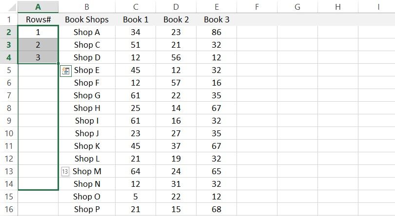
Select the first cell in the range that you want to fill.
Type the starting value for the series.
Type a value in the next cell to establish a pattern.

Tip: For example, if you want the series 1, 2, 3, 4, 5…, type 1 and 2 in the first two cells. If you want the series 2, 4, 6, 8…, type 2 and 4.
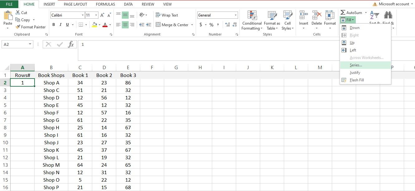
Select the cells that contain the starting values.

Note: In Excel 2013 and later, the Quick Analysis button is displayed by default when you select more than one cell containing data. You can ignore the button to complete this procedure.
Drag the fill handle across the range that you want to fill.

Note: As you drag the fill handle across each cell, Excel displays a preview of the value. If you want a different pattern, drag the fill handle by holding down the right-click button, and then choose a pattern.

To fill in increasing order, drag down or to the right. To fill in decreasing order, drag up or to the left.

Tip: If you do not see the fill handle, you may have to display it first. For more information, see Display or hide the fill handle.

Note: These numbers are not automatically updated when you add, move, or remove rows. You can manually update the sequential numbering by selecting two numbers that are in the right sequence, and then dragging the fill handle to the end of the numbered range.

Use the ROW function to number rows

In the first cell of the range that you want to number, type =ROW(A1).

The ROW function returns the number of the row that you reference. For example, =ROW(A1) returns the number 1.
Drag the fill handle across the range that you want to fill.

Tip: If you do not see the fill handle, you may have to display it first. For more information, see Display or hide the fill handle.

These numbers are updated when you sort them with your data. The sequence may be interrupted if you add, move, or delete rows. You can manually update the numbering by selecting two numbers that are in the right sequence, and then dragging the fill handle to the end of the numbered range.
If you are using the ROW function, and you want the numbers to be inserted automatically as you add new rows of data, turn that range of data into an Excel table. All rows that are added at the end of the table are numbered in sequence. For more information, see Create or delete an Excel table in a worksheet.

To enter specific sequential number codes, such as purchase order numbers, you can use the ROW function together with the TEXT function. For example, to start a numbered list by using 000-001, you enter the formula =TEXT(ROW(A1),»000-000″) in the first cell of the range that you want to number, and then drag the fill handle to the end of the range.

Display or hide the fill handle

The fill handle displays by default, but you can turn it on or off.

In Excel 2010 and later, click the File tab, and then click Options.

In Excel 2007, click the Microsoft Office Button , and then click Excel Options.
In the Advanced category, under Editing options, select or clear the Enable fill handle and cell drag-and-drop check box to display or hide the fill handle.

Note: To help prevent replacing existing data when you drag the fill handle, ensure the Alert before overwriting cells check box is selected. If you do not want Excel to display a message about overwriting cells, you can clear this check box.

Example

You’ll most probably need to number rows in Excel for serial numbering in your dataset so here’s an example of where it can be applied:

We have an employee database of a school which can do with some sequential numbering. Our aim is to serially number this dataset in column B.

With some methods, you will get static numbering of rows and dynamic numbering with the rest. If that is important to you, we’ve mentioned which method delivers which results with the subheadings.

Let’s get numbering!

Using Fill Handle

Static numbering

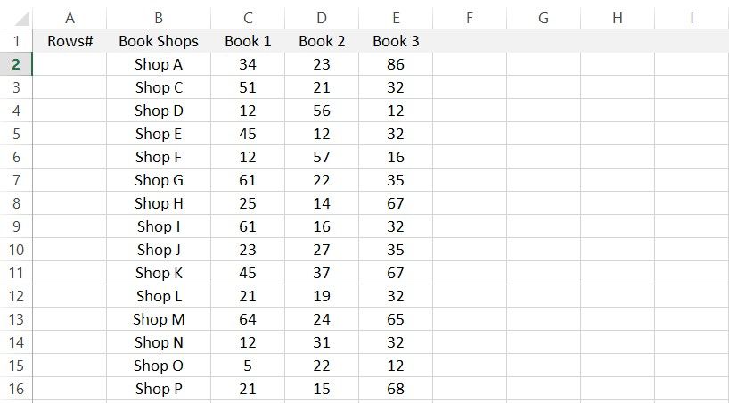
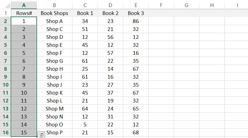
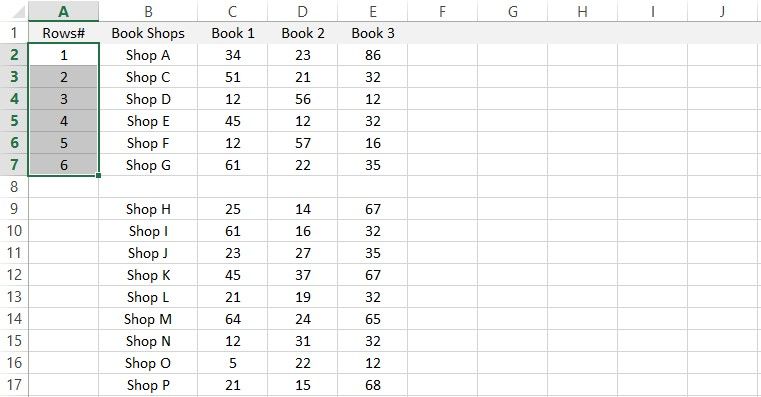
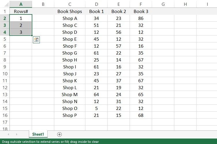
Let’s use the simplest method first which requires no functions or fancy features. We use the Fill Handle. The Fill Handle is the tiny square that appears at the bottom-right corner of the selected cell(s). The Fill Handle recognizes the formula or pattern contained in the selected cell(s) and copies them down to the extended range. With this feature, we can number the rows in our dataset. See below how it’s done:

In the column where you want the serial numbers, enter 1 and 2 in the first and second rows:

This will help the Fill Handle pick up on the pattern.
Select these two cells containing the numbers 1 and 2. The Fill Handle will appear in the bottom corner.

Hover the cursor on the Fill Handle until the cursor changes to a cross.

Now click and drag the Fill Handle to where you want the numbered rows. We want the rows numbered to 10 so we’ll drag the handle down to B12. The callout bubble will display the value for the target cell as you click and drag.

If you want to number the entire dataset’s rows, double-click the Fill Handle and it will number all the rows of the dataset that have the adjacent column filled.

When you release the left mouse button, the cells will be auto-filled with the numbered rows using the Fill Handle:

Using Fill Series Option

Static numbering

Here’s another feature that acts as a filler. To fill the rows with serial numbers, you can give Fill Series a go. Given its few options, you’ll find it quite handy for filling in numbers and dates in the specified steps. For now, we only need sequential numbering so we’ll head onto the steps right away:

Enter the number 1 in the first row of the column you want numbered.
Select the cell so that Fill Series can create the series to fill the column based on this number.
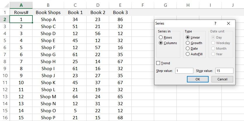
Select the Fill icon in the Editing section of the Home tab and then select the Series option from the menu.

The Series dialog box will be launched.
In the dialog box make the following selections:
- Select the Columns radio button in the Series in section
- Select the Linear radio button in the Type
- Enter the Step value and Stop value for your number series.
For us, that would be 1 and 10.
The Step value is the number by which you want the numbers to increase. E.g. if we enter 2 here, the numbers in the series would go 1, 3, 5….. Since we want regular numbering, we have entered 1 as the Step value.
Stop value is the number where you want the series to end.

Click on the OK button when done.

With these steps, the column will be filled with the given number series:

Incrementing Previous Row Number by 1

Static numbering

Now we move on to the formulas for numbering rows in Excel and it only makes sense to start with the simplest one first. By adding 1 to the previous row number, we can create a sequence of numbers. Here’s what you need to do if you choose this method:

Start by entering «1» in the first cell where the serial numbers will be.
In the next cell of the column, add 1 to the previous cell using this formula:

=B3+1

In this formula, B3 will be the cell containing the number 1. Adding 1 to B3 will result in the number 2. And this is how it will keep going. The next cell will be B4+1 which will result in 3, so on and so forth. In this way, the numbers will keep increasing serially.

Now extend the formula to where you want the last number.
With this plain arithmetic formula, the rows will be numbered up to 10:

Using ROW Function

Dynamic numbering

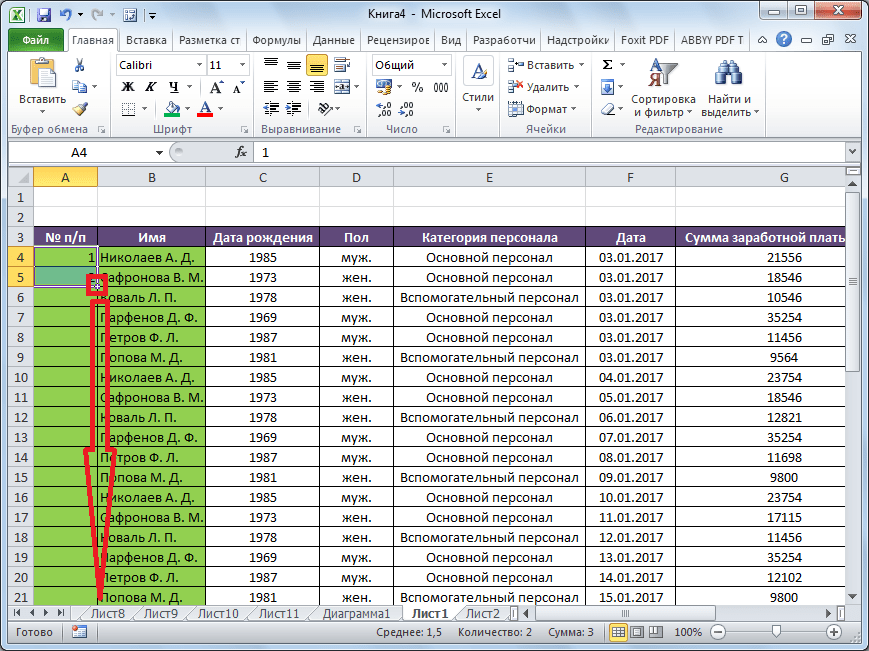
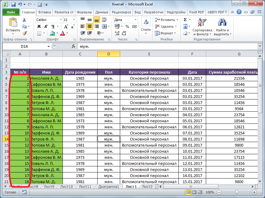
And now we will number rows using a simple function, the ROW function. The ROW function returns the row number of a referred cell. So, no matter where we are on the active worksheet, if you refer a certain cell, the ROW function would return the specified cell’s row number. With the steps below, we’ll show you how we make the ROW function work for returning numbered rows:

=ROW()-2

The ROW function has been used on its own to return the number of the row the formula is entered in and then we deduct that figure by 2. Why? Our target cell is B3 so =ROW() would return 3. To make the ROW function return 1 as the first number, we have deducted 2 in the formula. You will need to adjust this value according to the row your target cell is in.

As the formula is copied down, it will return the row number and then 2 will be subtracted. E.g. in the next instance, the row number is 4. 4-2 = 2. The next row number will be 5. 5-2 = 3 and so on.

We have chosen this formula since our numbering was starting from B3. If you’re already starting from row 1, you can enter the formula as:

=ROW()

This formula will return the row number of the cell the formula is entered in.

Note: Both the ROW formulas suggested above will bring about dynamic results that recalculate with additions and deletions.

Using COUNTA Function

Dynamic numbering

Going good up until now. Rows are being numbered, the morning birds are taking their cue and the sun is rising somewhere. And then you realize that as opposed to a continuous dataset, your data has some blank rows that don’t need numbering. Challenge accepted; we have the COUNTA function at our disposal.

The COUNTA function counts the number of cells in a range that are not empty. COUNTA will count the non-empty cells in the adjacent column and, with the IF and ISBLANK functions, will return nothing if the adjacent cell is blank. Sounds like a plan. Let’s see all the works. we begin with this formula:

=IF(ISBLANK(C3),"",COUNTA($C$3:C3))

As per the IF function, C3 will be checked by the ISBLANK function as to whether it’s a blank cell or not. If this tests true, the IF function will return an empty text string «».

If the cell is not blank, then the COUNTA function will start counting the non-blank cells from $C$3 (mentioning the number as an absolute reference locks the cell in the formula so that as the formula is copied down, the reference remains the same) and return the count as the answer of the formula.

In the first instance, the count from C3 only makes 1 cell so 1 is the result.

In the next instance, COUNT counts C3 and C4 and therefore returns 2. In the third instance, the adjacent cell i.e. C5 is blank so this row has not been numbered.

Note: The results of using this formula are dynamic; with any change of addition or deletion of data, the numbering will recalculate and adjust accordingly.

Using OFFSET Function

Dynamic numbering

Rows in Excel can also be numbered using the OFFSET function. It’s a slightly “off” the norm method but a method nonetheless and it requires you to start the column without a header; you’ll see why in a while.

The OFFSET function returns the value of the cell which is the given numbers of rows and columns from the specified cell. We will use this concept to then add 1 to each result to create serial numbering. Below is the demonstration with the formula:

=OFFSET(B3,-1,0)+1

Now you’ll see why a blank column header was a prerequisite. Let’s understand the path in the formula. The cell specified is B3 itself. From there, OFFSET trails to -1 rows. This means B2. now in the third parameter of the formula, from B2 we need to shift to 0 columns which still leads to B2.

This means that using the OFFSET function, we will be referring to the previous cell in the same column. In the last bit of the formula, we have +1 which adds the number 1 to the value of B2. Since B2 is blank, 0+1 = 1. 1 is the outcome here. This is why we needed the header to be blank.

In the next instance, OFFSET will lead to B3 and add 1 to B3’s value. 1+1 = 2. That is how the rest of the rows will be numbered in succession.

Once you are done, you can copy and paste the values over themselves and add the column header if you so wish. The values are pasted back so that they are not formula-reliant and won’t cause errors.

Note: As long as the column header is absent, the results of this formula are dynamic. If you wish to add the column header, you will have to paste back the values or you can choose another method if want to retain the column header and the dynamic numbering.

Using SUBTOTAL Function

Dynamic numbering

And again, things were looking bright until you were hit with another requirement. You need to filter data but that would also filter the serial numbers. Now that’s a problem but not a problem we can’t work around. Enter SUBTOTAL function.

The SUBTOTAL function returns a subtotal in a dataset. While we will be using the COUNTA function via SUBTOTAL, SUBTOTAL will help to dynamically recalculate the row numbers as the data is filtered. Want to see how that works? We’ve got the formula to number rows with the SUBTOTAL function right ahead:

=SUBTOTAL(3,$C$3:C3)

The SUBTOTAL function presents a list of functions to choose from in the Formula AutoComplete. This parameter will determine what kind of subtotal you want to enter.

After selecting the function, the next input is the cell reference. As shown in the COUNTA function section above, we will enter $C$3:C3 as the range so that the count always begins from $C$3. As the formula is filled downward, the count will continue up until the target cell.

Now try filtering your data.

The row numbers will be recalculated with the filtered data serially numbered:

With the new serial number selected, we can note in the formula that the count for non-blank cells has started from $C$3 to C4 instead of C3. In this way, the count will begin from $C$3 and jump directly to the first filtered cell in the C column.

Creating Calculated Column in Excel Table

Dynamic numbering

Last but not least, let’s table it! An Excel table talks the talk and walks the walk and there are many convenient features it offers. The one helping us today is a calculated column; enter one formula and you’ll have numbered rows. Excel tables are known for being dynamic in their very nature and a calculated column also provides that ease. Nothing short of Excel magic. The complete tricks (read steps) to do this are as follows:

Select any cell in the dataset. This will help Excel identify the range to create the Excel table.
In the Home tab, go to the Styles section and click on the Format as a Table Select the table style from the menu or create your own.

Now a small dialog box will appear confirming the identified range of the intended Excel table. Correct the range if required.
If your table has headers, leave the My table has headers checkbox checked.
Then click on the OK button to close the dialog box and apply the table.

An Excel table will be created on the provided range:

Now, enter this formula in any cell in the column where you want the numbers:

=ROW()-ROW(Table1[#Headers])

As a calculated column, when the formula is entered, all the rows will automatically be serially numbered:

And that’s your job done!

And that’s our tutorial done! The solutions may be numbered but so are the problems and today you saw how to tackle numbering rows in Excel in many different ways.

Filtering data and dealing with gaps in the data are two hitches you might face when numbering rows but today you’ve learned how to breeze through them. We’re up for making other hitches easy, breezy and we’re on it too so we’ll see you around another Excel trick!

Источник

Watch Video – 7 Quick and Easy Ways to Number Rows in Excel

When working with Excel, there are some small tasks that need to be done quite often. Knowing the ‘right way’ can save you a great deal of time.

One such simple (yet often needed) task is to number the rows of a dataset in Excel (also called the serial numbers in a dataset).

Now if you’re thinking that one of the ways is to simply enter these serial number manually, well – you’re right!

But that’s not the best way to do it.

Imagine having hundreds or thousands of rows for which you need to enter the row number. It would be tedious – and completely unnecessary.

There are many ways to number rows in Excel, and in this tutorial, I am going to share some of the ways that I recommend and often use.

Of course, there would be more, and I will be waiting – with a coffee – in the comments area to hear from you about it.

The best way to number the rows in Excel would depend on the kind of data set that you have.

For example, you may have a continuous data set that starts from row 1, or a dataset that start from a different row. Or, you might have a dataset that has a few blank rows in it, and you only want to number the rows that are filled.

You can choose any one of the methods that work based on your dataset.

1] Using Fill Handle

Fill handle identifies a pattern from a few filled cells and can easily be used to quickly fill the entire column.

Suppose you have a dataset as shown below:

Here are the steps to quickly number the rows using the fill handle:

Note that Fill Handle automatically identifies the pattern and fill the remaining cells with that pattern. In this case, the pattern was that the numbers were getting incrementing by 1.

In case you have a blank row in the dataset, fill handle would only work till the last contiguous non-blank row.

Also, note that in case you don’t have data in the adjacent column, double-clicking the fill handle would not work. You can, however, place the cursor on the fill handle, hold the right mouse key and drag down. It will fill the cells covered by the cursor dragging.

2] Using Fill Series

While Fill Handle is a quick way to number rows in Excel, Fill Series gives you a lot more control over how the numbers are entered.

Suppose you have a dataset as shown below:

Here are the steps to use Fill Series to number rows in Excel:

This will instantly number the rows from 1 to 26.

Using ‘Fill Series’ can be useful when you’re starting by entering the row numbers. Unlike Fill Handle, it doesn’t require the adjacent columns to be filled already.

Even if you have nothing on the worksheet, Fill Series would still work.

Note: In case you have blank rows in the middle of the dataset, Fill Series would still fill the number for that row.

3] Using the ROW Function

You can also use Excel functions to number the rows in Excel.

In the Fill Handle and Fill Series methods above, the serial number inserted is a static value. This means that if you move the row (or cut and paste it somewhere else in the dataset), the row numbering will not change accordingly.

This shortcoming can be tackled using formulas in Excel.

You can use the ROW function to get the row numbering in Excel.

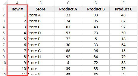
To get the row numbering using the ROW function, enter the following formula in the first cell and copy for all the other cells:

=ROW()-1

The ROW() function gives the row number of the current row. So I have subtracted 1 from it as I started from the second row onwards. If your data starts from the 5th row, you need to use the formula =ROW()-4.

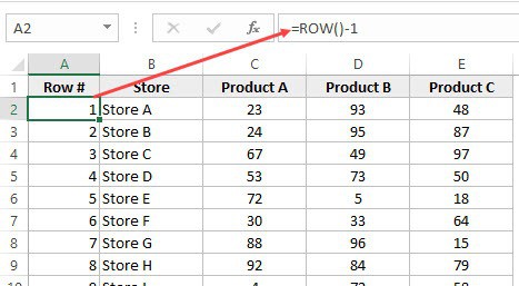
The best part about using the ROW function is that it will not screw up the numberings if you delete a row in your dataset.

Since the ROW function is not referencing any cell, it will automatically (or should I say AutoMagically) adjust to give you the correct row number. Something as shown below:

Note that as soon as I delete a row, the row numbers automatically update.

Again, this would not take into account any blank records in the dataset. In case you have blank rows, it will still show the row number.

You can use the following formula to hide the row number for blank rows, but it would still not adjust the row numbers (such that the next row number is assigned to the next filled row).

IF(ISBLANK(B2),"",ROW()-1)

4] Using the COUNTA Function

If you want to number rows in a way that only the ones that are filled get a serial number, then this method is the way to go.

It uses the COUNTA function that counts the number of cells in a range that are not empty.

Suppose you have a dataset as shown below:

Note that there are blank rows in the above-shown dataset.

Here is the formula that will number the rows without numbering the blank rows.

=IF(ISBLANK(B2),"",COUNTA($B$2:B2))

The IF function checks whether the adjacent cell in column B is empty or not. If it’s empty, it returns a blank, but if it’s not, it returns the count of all the filled cells till that cell.

5] Using SUBTOTAL For Filtered Data

Sometimes, you may have a huge dataset, where you want to filter the data and then copy and paste the filtered data into a separate sheet.

If you use any of the methods shown above so far, you will notice that the row numbers remain the same. This means that when you copy the filtered data, you will have to update the row numbering.

In such cases, the SUBTOTAL function can automatically update the row numbers. Even when you filter the data set, the row numbers will remain intact.

Let me show you exactly how it works with an example.

Suppose you have a dataset as shown below:

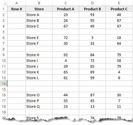
If I filter this data based on Product A sales, you will get something as shown below:

Note that the serial numbers in Column A are also filtered. So now, you only see the numbers for the rows that are visible.

While this is the expected behavior, in case you want to get a serial row numbering – so that you can simply copy and paste this data somewhere else – you can use the SUBTOTAL function.

Here is the SUBTOTAL function that will make sure that even the filtered data has continuous row numbering.

=SUBTOTAL(3,$B$2:B2)

The 3 in the SUBTOTAL function specifies using the COUNTA function. The second argument is the range on which COUNTA function is applied.

The benefit of the SUBTOTAL function is that it dynamically updates when you filter the data (as shown below):

Note that even when the data is filtered, the row numbering update and remains continuous.

6] Creating an Excel Table

Excel Table is a great tool that you must use when working with tabular data. It makes managing and using data a lot easier.

This is also my favorite method among all the techniques shown in this tutorial.

Let me first show you the right way to number the rows using an Excel Table:

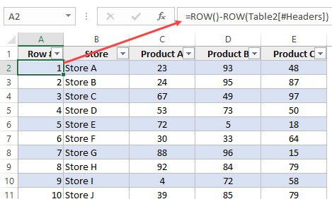
Note that in the formula above, I have used Table2, as that is the name of my Excel table. You can replace Table2 with the name of the table you have.

There are some added benefits of using an Excel Table while numbering rows in Excel:

Since Excel Table automatically inserts the formula in the entire column, it works when you insert a new row in the Table. This means that when you insert/delete rows in an Excel Table, the row numbering would automatically update (as shown below).
If you add more rows to the data, Excel Table would automatically expand to include this data as a part of the table. And since the formulas automatically update in the calculated columns, it would insert the row number for the newly inserted row (as shown below).

7] Adding 1 to the Previous Row Number

This is a simple method that works.

The idea is to add 1 to the previous row number (the number in the cell above). This will make sure that subsequent rows get a number that is incremented by 1.

Suppose you have a dataset as shown below:

Here are the steps to enter row numbers using this method:

In the cell in the first row, enter 1 manually. In this case, it’s in cell A2.
In cell A3, enter the formula, =A2+1
Copy and paste the formula for all the cells in the column.

The above steps would enter serial numbers in all the cells in the column. In case there are any blank rows, this would still insert the row number for it.

Also note that in case you insert a new row, the row number would not update. In case you delete a row, all the cells below the deleted row would show a reference error.

These are some quick ways you can use to insert serial numbers in tabular data in Excel.

In case you are using any other method, do share it with me in the comments section.

You May Also Like the Following Excel Tutorials:

Delete Blank Rows in Excel (with and without VBA).
How to Insert Multiple Rows in Excel (4 Methods).
How to Split Multiple Lines in a Cell into a Separate Cells / Columns.
7 Amazing Things Excel Text to Columns Can Do For You.
Highlight EVERY Other ROW in Excel.
How to Compare Two Columns in Excel.
Insert New Columns in Excel

Источник

Содержание

Способ 1: заполнение первых двух строк
Способ 2: использование функции
Способ 3: использование прогрессии
Вопросы и ответы

Программа Microsoft Excel предоставляет пользователям сразу несколько способов автоматической нумерации строк. Одни из них максимально просты, как в выполнении, так и в функционале, а другие – более сложные, но и заключают в себе большие возможности.

Способ 1: заполнение первых двух строк

Первый способ предполагает ручное заполнение первых двух строк числами.

В выделенной под нумерацию колонке первой строки ставим цифру – «1», во второй (той же колонки) – «2».

Выделяем эти две заполненные ячейки. Становимся на нижний правый угол самой нижней из них. Появляется маркер заполнения. Кликаем левой кнопкой мыши и с зажатой кнопкой, протягиваем его вниз до конца таблицы.

Как видим, нумерация строчек автоматически заполнилась по порядку.

Этот метод довольно легкий и удобный, но он хорош только для относительно небольших таблиц, так как тянуть маркер по таблице в несколько сотен, а то и тысяч строк, все-таки затруднительно.

Способ 2: использование функции

Второй способ автоматического заполнения предусматривает использование функции «СТРОКА».

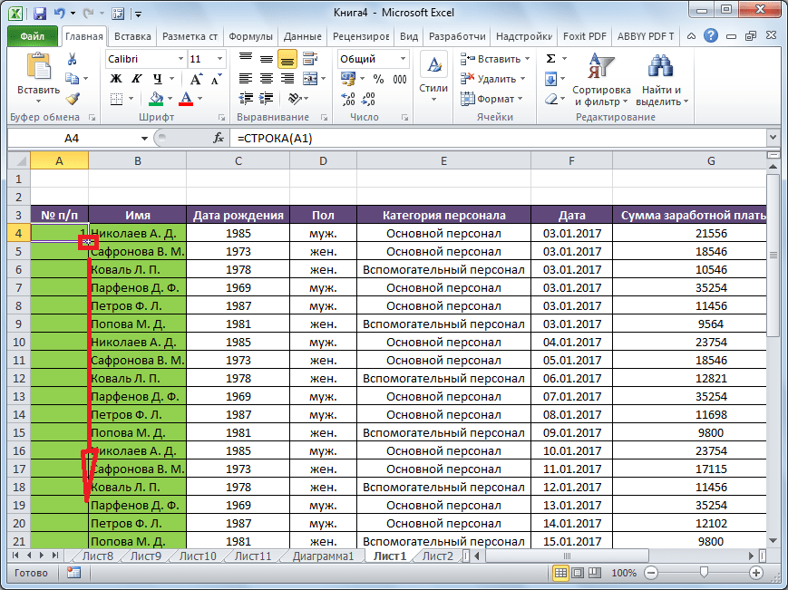
Выделяем ячейку, в которой будет находиться цифра «1» нумерации. Вводим в строку для формул выражение «=СТРОКА(A1)».Кликаем по клавише ENTER на клавиатуре.

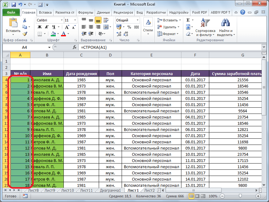
Как и в предыдущем случае, копируем с помощью маркера заполнения формулу в нижние ячейки таблицы данного столбца. Только в этот раз выделяем не две первые ячейки, а только одну.

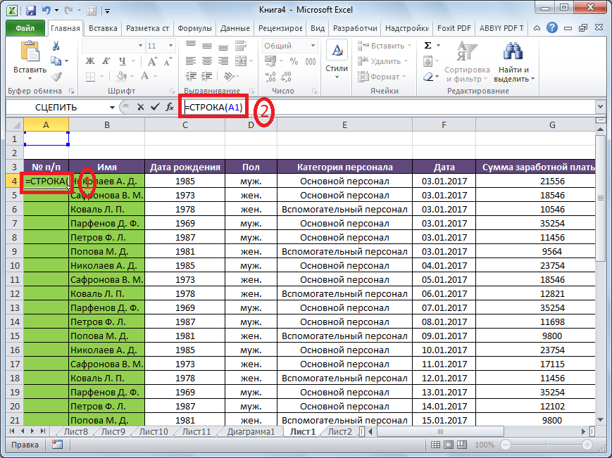
Как видим, нумерация строк и в этом случае расположилась по порядку.

Но, по большому счету, этот способ мало чем отличается от предыдущего и не решает проблему с потребностью тащить маркер через всю таблицу.

Способ 3: использование прогрессии

Как раз третий способ нумерации с использованием прогрессии подойдет для длинных таблиц с большим количеством строк.

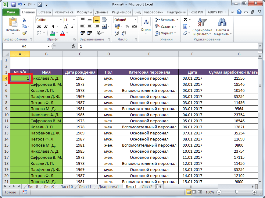
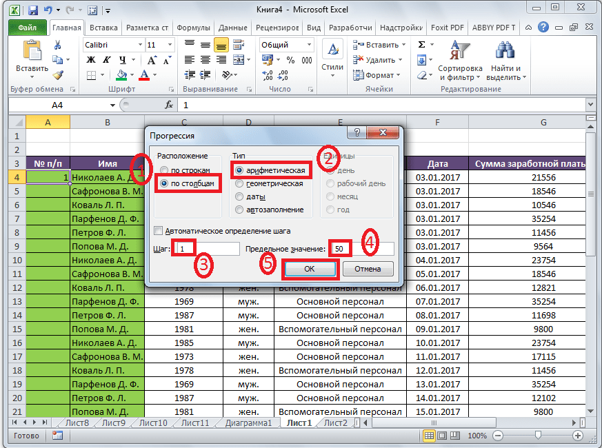
Первую ячейку нумеруем самым обычным способом, вписав туда цифру «1» с клавиатуры.

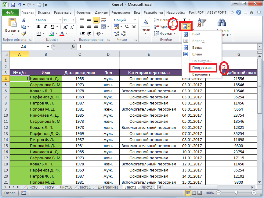
На ленте в блоке инструментов «Редактирование», который расположен во вкладке «Главная», жмем на кнопку «Заполнить». В появившемся меню кликаем по пункту «Прогрессия».

Открывается окно «Прогрессия». В параметре «Расположение» нужно установить переключатель в позицию «По столбцам». Переключатель параметра «Тип» должен находиться в позиции «Арифметическая». В поле «Шаг» нужно установить число «1», если там установлено другое. Обязательно заполните поле «Предельное значение». Тут следует указать количество строк, которые нужно пронумеровать. Если данный параметр не заполнен, автоматическая нумерация произведена не будет. В конце следует нажать на кнопку «OK».

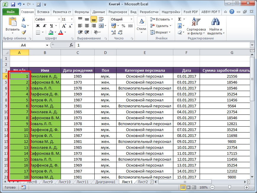
Как видим, поле этого все строки вашей таблицы будут пронумерованы автоматически. В этом случае даже ничего перетягивать не придется.

Как альтернативный вариант можно использовать следующую схему этого же способа:

В первой ячейке поставить цифру «1», а затем выделить весь диапазон ячеек, которые вы хотите пронумеровать.

Вызвать окно инструмента «Прогрессия» тем же способом, о котором мы говорили выше. Но на этот раз ничего вводить или изменять не нужно. В том числе, вводить данные в поле «Предельное значение» не придется, так как нужный диапазон уже выделен. Достаточно просто нажать на кнопку «OK».

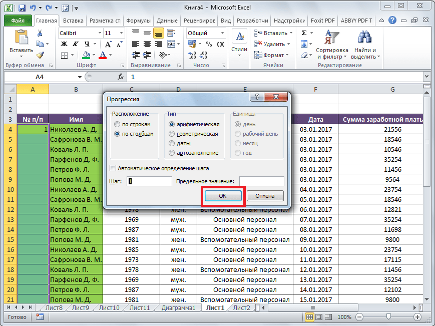
Данный вариант хорош тем, что вам не придется прикидывать, из скольких строк состоит таблица. В то же время, вам нужно будет выделять все ячейки столбца с номерами, а это значит, что мы возвращаемся к тому же, что было при использовании первых способов: к необходимости прокручивать таблицу до самого низа.

Как видим, существует три основных способа автоматической нумерации строк в программе. Из них наибольшую практическую ценность имеет вариант с нумерацией первых двух строк с последующим копированием (как самый простой) и вариант с использованием прогрессии (из-за возможности работать с большими таблицами).

Еще статьи по данной теме:

Помогла ли Вам статья?

Источник

Unlike other Microsoft Office programs, Excel doesn’t provide a direct function to number data automatically. Here are 3 easy ways to do it.

Formatting data in Microsoft Excel can be tricky, especially when you need to amend a large dataset already filled out. Numbering the rows in Excel is an example of such formatting.

If a dataset is small and continuous, one can easily number its rows manually or by auto-filling sequence. When the dataset is large and inconsistent, some data needs to be added or removed from the middle, or when you need to filter the data in a specific column, the numbering gets messed up.

Let’s explore different ways to number rows of the consistent and inconsistent (empty rows) datasets in Microsoft Excel.

1. Numbering Rows of a Consistent Dataset in Excel Using Fill Handle and Fill Series:

Using the Fill Handle or Fill Series is the easiest way to number rows when you have a consistent dataset with no empty rows.

For better understanding, let’s apply both ways of numbering rows to a dataset shown below:

To number rows with Fill Handle, follow these steps:

Put 1, 2, and 3 in cells A2, A3, and A4.
Select the cells A2 through A4.
A plus icon will appear in the bottom-right corner of the last selected cell when your cursor hovers over it.
Clicking twice on it will number all the continuous rows below it.

Therefore, if no empty rows appear throughout the dataset, it is a fast method for numbering rows. However, Fill Handle does not work in these two cases:

Whenever the Fill Handle encounters an inconsistency (an empty row), it will automatically stop.
If the adjacent column where you are using Fill Handle is empty, it won’t work.

However, there is a workaround to this, namely manual auto-filling of the sequence. In this way, even if there is an inconsistency in the dataset or the adjacent column is empty, you can still number the rows all the way to the end.

Auto-filling is as simple as dragging the lower-right corner of selected cells where the plus sign is displayed and extending it to the end.

But this method is not viable due to the following reasons:

It also numbers any empty rows that come in its way, which of course, we do not want.
Manually dragging a dataset to the bottom becomes problematic if the dataset is extensive.

Alternatively, you can use the Fill Series method if you do not want to manually drag sequences in a large dataset but still want auto-fill data to the end. Let’s look at how it works.

Note the total number of filled rows in the dataset by pressing CTRL + End.
In cell A2, enter 1.
Select Series from the Fill dropdown in the Editing section of the Home tab.
Choose Columns in Series in and Linear in Type.
Set Stop value to the total number of filled rows and Step value to 1.
Click OK.

The rows will be automatically numbered up to the last filled one, including the empty ones. Although it eliminates manual dragging and does not stop filling at the empty row, it won’t work when making professional spreadsheets since it numbers empty rows, which we don’t want.

Furthermore, since both methods are static, if you delete a row and move or replace it, you will have to renumber it. Nevertheless, both methods are easy to use and work well when the data is consistent.

Let’s look at how to number inconsistent datasets with empty rows using the COUNTA and IF functions.

2. Using COUNTA and IF Functions to Number Rows in an Inconsistent Dataset

The COUNTA function skips empty rows while numbering the filled ones in sequence. To see how it works, let’s apply it to an inconsistent dataset:

Consider the following dataset:
Fill in the following formula in cell A2:
```
=IF(ISBLANK(B2),"",COUNTA($B$2:B2))
```
Using auto-fill, fill in the remaining cells below.

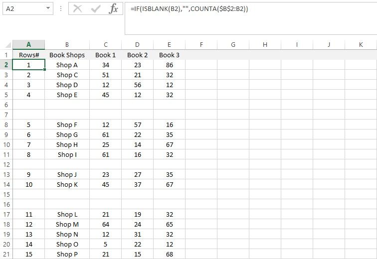
You can see that it skipped over the empty cells while numbered only the filled ones in order. Here, the IF function decides whether the adjacent cell is empty. It leaves the rows empty if adjacent cells are empty and count them if they are filled.

Moreover, this method of numbering rows is dynamic, so when you add, replace, or remove a row, the numbering will automatically be updated.

However, what if you need to fill the dataset and want to maintain the row numbers? In this case, the combination of IF and COUNTA won’t help, and neither will Fill Handle or Fill Series.

Then you can go for another approach, using the SUBTOTAL function to maintain row numbering in the datasheet while filtering data.

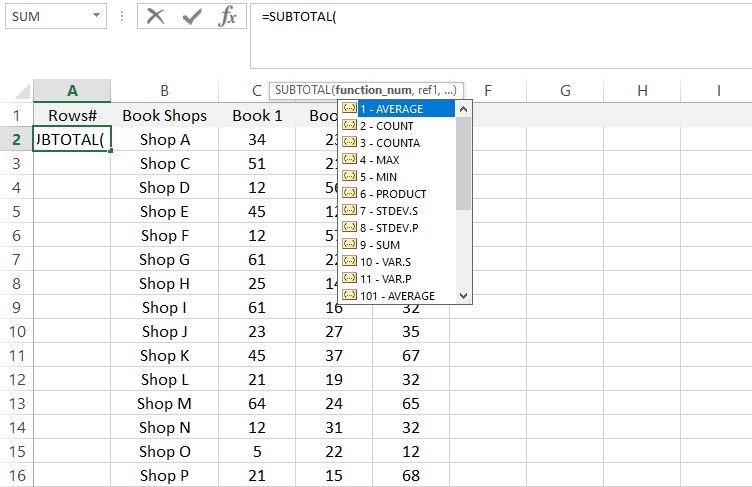
3. Using SUBTOTAL Function

Let’s view the SUBTOTAL function syntax before we apply it to the dataset.

=SUBTOTAL(function_num, range 1, [range 2..])

Range 1 indicates the range of the dataset where the function is to be applied. The function_num indicates where your desired function is located in the list, as shown below.

To number rows using SUBTOTAL, follow these steps:

Go to cell A2.
There, enter the following formula:
```
=SUBTOTAL(3,B2:$B$2)
```
Fill in the sequence to populate entries in the cells below.

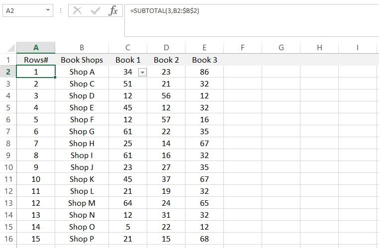
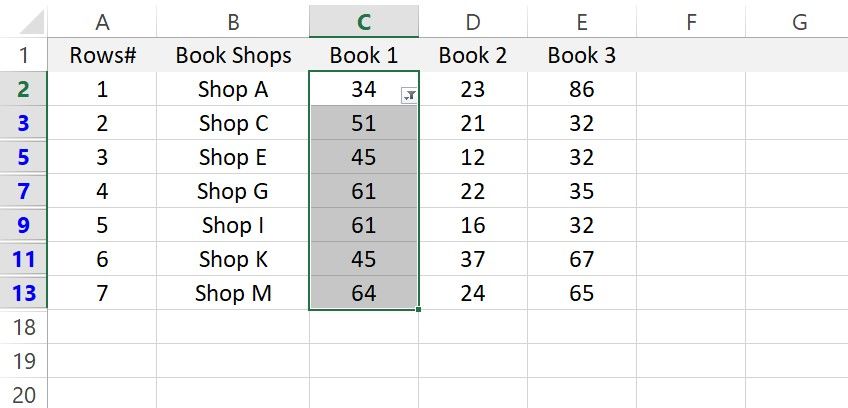
Now, as shown below, when you filter the data in any other column, the row numbering will change automatically in the correct order.

Comparing the Uses of Each Method

Let’s briefly review where all three methods are useful:

As long as you have consistent data with no empty rows, you can use Fill Handle or Fill Series to number the rows.
If the data is inconsistent, and you only need to number the rows (without filtering them later), you can use the second method of combining the COUNTA function with an IF function.
The SUBTOTAL function will work whenever you need to filter data while maintaining row numbering.

Number Rows With Ease in Microsoft Excel

This way, no matter if the data is consistent or not, you can easily number the rows. Choose whichever method best suits your needs.

Besides these three methods, you can also use the ROW function and create an Excel table to number rows, but each of these approaches has its limitations.

Is it always a struggle to manage multiple worksheets with endless rows and columns? You can easily group rows and columns, so the data is easier for you to handle and easier for your clients and colleagues to navigate. Use them in your spreadsheets to make them look more professional.

Источник

How to number rows in excel

Automatically number rows

What do you want to do?

Fill a column with a series of numbers

Use the ROW function to number rows

Display or hide the fill handle

See Also

Need more help?

Want more options?

Example

Using Fill Handle

Using Fill Series Option

Incrementing Previous Row Number by 1

Using ROW Function

Using COUNTA Function

Using OFFSET Function

Using SUBTOTAL Function

Creating Calculated Column in Excel Table