
Automatically number rows
Unlike other Microsoft 365 programs, Excel does not provide a button to number data automatically. But, you can easily add sequential numbers to rows of data by dragging the fill handle to fill a column with a series of numbers or by using the ROW function.
Tip: If you are looking for a more advanced auto-numbering system for your data, and Access is installed on your computer, you can import the Excel data to an Access database. In an Access database, you can create a field that automatically generates a unique number when you enter a new record in a table.

What do you want to do?
-
Fill a column with a series of numbers
-
Use the ROW function to number rows
-
Display or hide the fill handle
Fill a column with a series of numbers
-
Select the first cell in the range that you want to fill.
-
Type the starting value for the series.
-
Type a value in the next cell to establish a pattern.
Tip: For example, if you want the series 1, 2, 3, 4, 5…, type 1 and 2 in the first two cells. If you want the series 2, 4, 6, 8…, type 2 and 4.
-
Select the cells that contain the starting values.
Note: In Excel 2013 and later, the Quick Analysis button is displayed by default when you select more than one cell containing data. You can ignore the button to complete this procedure.
-
Drag the fill handle
 across the range that you want to fill.
Note: As you drag the fill handle across each cell, Excel displays a preview of the value. If you want a different pattern, drag the fill handle by holding down the right-click button, and then choose a pattern.
To fill in increasing order, drag down or to the right. To fill in decreasing order, drag up or to the left.
Tip: If you do not see the fill handle, you may have to display it first. For more information, see Display or hide the fill handle.
Note: These numbers are not automatically updated when you add, move, or remove rows. You can manually update the sequential numbering by selecting two numbers that are in the right sequence, and then dragging the fill handle to the end of the numbered range.
Use the ROW function to number rows
-
In the first cell of the range that you want to number, type =ROW(A1).
The ROW function returns the number of the row that you reference. For example, =ROW(A1) returns the number 1.
-
Drag the fill handle
across the range that you want to fill.Tip: If you do not see the fill handle, you may have to display it first. For more information, see Display or hide the fill handle.
-
These numbers are updated when you sort them with your data. The sequence may be interrupted if you add, move, or delete rows. You can manually update the numbering by selecting two numbers that are in the right sequence, and then dragging the fill handle to the end of the numbered range.
-
If you are using the ROW function, and you want the numbers to be inserted automatically as you add new rows of data, turn that range of data into an Excel table. All rows that are added at the end of the table are numbered in sequence. For more information, see Create or delete an Excel table in a worksheet.
To enter specific sequential number codes, such as purchase order numbers, you can use the ROW function together with the TEXT function. For example, to start a numbered list by using 000-001, you enter the formula =TEXT(ROW(A1),»000-000″) in the first cell of the range that you want to number, and then drag the fill handle to the end of the range.
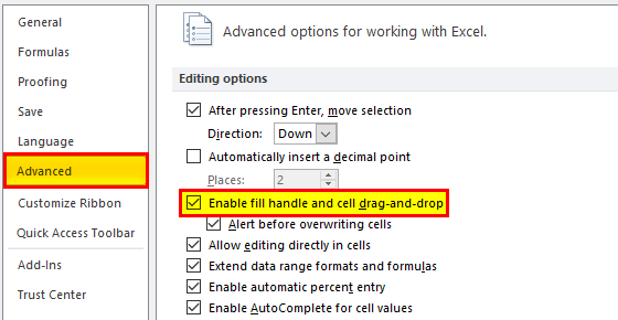
Display or hide the fill handle
The fill handle  displays by default, but you can turn it on or off.
-
In Excel 2010 and later, click the File tab, and then click Options.
In Excel 2007, click the Microsoft Office Button
, and then click Excel Options. -
In the Advanced category, under Editing options, select or clear the Enable fill handle and cell drag-and-drop check box to display or hide the fill handle.
 , and then click Excel Options.
Note: To help prevent replacing existing data when you drag the fill handle, ensure the Alert before overwriting cells check box is selected. If you do not want Excel to display a message about overwriting cells, you can clear this check box.
See Also
Overview of formulas in Excel
How to avoid broken formulas
Find and correct errors in formulas
Excel keyboard shortcuts and function keys
Lookup and reference functions (reference)
Excel functions (alphabetical)
Excel functions (by category)
Need more help?
Watch Video – 7 Quick and Easy Ways to Number Rows in Excel
When working with Excel, there are some small tasks that need to be done quite often. Knowing the ‘right way’ can save you a great deal of time.
One such simple (yet often needed) task is to number the rows of a dataset in Excel (also called the serial numbers in a dataset).
Now if you’re thinking that one of the ways is to simply enter these serial number manually, well – you’re right!
But that’s not the best way to do it.
Imagine having hundreds or thousands of rows for which you need to enter the row number. It would be tedious – and completely unnecessary.
There are many ways to number rows in Excel, and in this tutorial, I am going to share some of the ways that I recommend and often use.
Of course, there would be more, and I will be waiting – with a coffee – in the comments area to hear from you about it.
How to Number Rows in Excel
The best way to number the rows in Excel would depend on the kind of data set that you have.
For example, you may have a continuous data set that starts from row 1, or a dataset that start from a different row. Or, you might have a dataset that has a few blank rows in it, and you only want to number the rows that are filled.
You can choose any one of the methods that work based on your dataset.
1] Using Fill Handle
Fill handle identifies a pattern from a few filled cells and can easily be used to quickly fill the entire column.
Suppose you have a dataset as shown below:

Here are the steps to quickly number the rows using the fill handle:
Note that Fill Handle automatically identifies the pattern and fill the remaining cells with that pattern. In this case, the pattern was that the numbers were getting incrementing by 1.
In case you have a blank row in the dataset, fill handle would only work till the last contiguous non-blank row.
Also, note that in case you don’t have data in the adjacent column, double-clicking the fill handle would not work. You can, however, place the cursor on the fill handle, hold the right mouse key and drag down. It will fill the cells covered by the cursor dragging.
2] Using Fill Series
While Fill Handle is a quick way to number rows in Excel, Fill Series gives you a lot more control over how the numbers are entered.
Suppose you have a dataset as shown below:
Here are the steps to use Fill Series to number rows in Excel:
This will instantly number the rows from 1 to 26.
Using ‘Fill Series’ can be useful when you’re starting by entering the row numbers. Unlike Fill Handle, it doesn’t require the adjacent columns to be filled already.
Even if you have nothing on the worksheet, Fill Series would still work.
Note: In case you have blank rows in the middle of the dataset, Fill Series would still fill the number for that row.
3] Using the ROW Function
You can also use Excel functions to number the rows in Excel.
In the Fill Handle and Fill Series methods above, the serial number inserted is a static value. This means that if you move the row (or cut and paste it somewhere else in the dataset), the row numbering will not change accordingly.
This shortcoming can be tackled using formulas in Excel.
You can use the ROW function to get the row numbering in Excel.
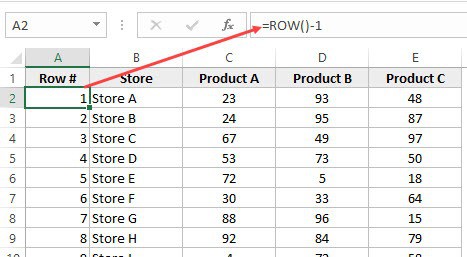
To get the row numbering using the ROW function, enter the following formula in the first cell and copy for all the other cells:
=ROW()-1
The ROW() function gives the row number of the current row. So I have subtracted 1 from it as I started from the second row onwards. If your data starts from the 5th row, you need to use the formula =ROW()-4.
The best part about using the ROW function is that it will not screw up the numberings if you delete a row in your dataset.
Since the ROW function is not referencing any cell, it will automatically (or should I say AutoMagically) adjust to give you the correct row number. Something as shown below:

Note that as soon as I delete a row, the row numbers automatically update.
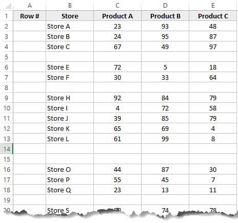
Again, this would not take into account any blank records in the dataset. In case you have blank rows, it will still show the row number.
You can use the following formula to hide the row number for blank rows, but it would still not adjust the row numbers (such that the next row number is assigned to the next filled row).
IF(ISBLANK(B2),"",ROW()-1)
4] Using the COUNTA Function
If you want to number rows in a way that only the ones that are filled get a serial number, then this method is the way to go.
It uses the COUNTA function that counts the number of cells in a range that are not empty.
Suppose you have a dataset as shown below:
Note that there are blank rows in the above-shown dataset.
Here is the formula that will number the rows without numbering the blank rows.
=IF(ISBLANK(B2),"",COUNTA($B$2:B2))
The IF function checks whether the adjacent cell in column B is empty or not. If it’s empty, it returns a blank, but if it’s not, it returns the count of all the filled cells till that cell.
5] Using SUBTOTAL For Filtered Data
Sometimes, you may have a huge dataset, where you want to filter the data and then copy and paste the filtered data into a separate sheet.
If you use any of the methods shown above so far, you will notice that the row numbers remain the same. This means that when you copy the filtered data, you will have to update the row numbering.
In such cases, the SUBTOTAL function can automatically update the row numbers. Even when you filter the data set, the row numbers will remain intact.
Let me show you exactly how it works with an example.
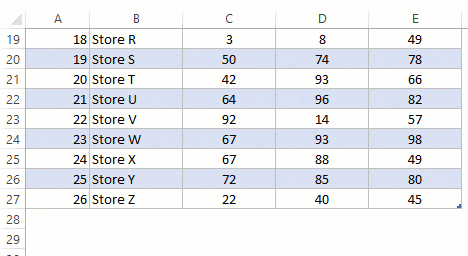
Suppose you have a dataset as shown below:

If I filter this data based on Product A sales, you will get something as shown below:

Note that the serial numbers in Column A are also filtered. So now, you only see the numbers for the rows that are visible.
While this is the expected behavior, in case you want to get a serial row numbering – so that you can simply copy and paste this data somewhere else – you can use the SUBTOTAL function.
Here is the SUBTOTAL function that will make sure that even the filtered data has continuous row numbering.
=SUBTOTAL(3,$B$2:B2)
The 3 in the SUBTOTAL function specifies using the COUNTA function. The second argument is the range on which COUNTA function is applied.
The benefit of the SUBTOTAL function is that it dynamically updates when you filter the data (as shown below):

Note that even when the data is filtered, the row numbering update and remains continuous.
6] Creating an Excel Table
Excel Table is a great tool that you must use when working with tabular data. It makes managing and using data a lot easier.
This is also my favorite method among all the techniques shown in this tutorial.
Let me first show you the right way to number the rows using an Excel Table:
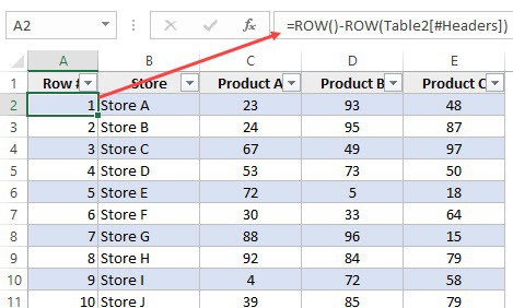
Note that in the formula above, I have used Table2, as that is the name of my Excel table. You can replace Table2 with the name of the table you have.
There are some added benefits of using an Excel Table while numbering rows in Excel:
- Since Excel Table automatically inserts the formula in the entire column, it works when you insert a new row in the Table. This means that when you insert/delete rows in an Excel Table, the row numbering would automatically update (as shown below).

- If you add more rows to the data, Excel Table would automatically expand to include this data as a part of the table. And since the formulas automatically update in the calculated columns, it would insert the row number for the newly inserted row (as shown below).


7] Adding 1 to the Previous Row Number
This is a simple method that works.
The idea is to add 1 to the previous row number (the number in the cell above). This will make sure that subsequent rows get a number that is incremented by 1.
Suppose you have a dataset as shown below:
Here are the steps to enter row numbers using this method:
- In the cell in the first row, enter 1 manually. In this case, it’s in cell A2.
- In cell A3, enter the formula, =A2+1
- Copy and paste the formula for all the cells in the column.

The above steps would enter serial numbers in all the cells in the column. In case there are any blank rows, this would still insert the row number for it.
Also note that in case you insert a new row, the row number would not update. In case you delete a row, all the cells below the deleted row would show a reference error.
These are some quick ways you can use to insert serial numbers in tabular data in Excel.
In case you are using any other method, do share it with me in the comments section.
You May Also Like the Following Excel Tutorials:
- Delete Blank Rows in Excel (with and without VBA).
- How to Insert Multiple Rows in Excel (4 Methods).
- How to Split Multiple Lines in a Cell into a Separate Cells / Columns.
- 7 Amazing Things Excel Text to Columns Can Do For You.
- Highlight EVERY Other ROW in Excel.
- How to Compare Two Columns in Excel.
- Insert New Columns in Excel
Numbering rows in Excel. Doesn’t sound like a tough feat, right? Don’t worry, it really isn’t. Why would you need to number rows? When handling any database, it can always do with organizing and the organizing may come in the form of alphabetical order, chronological order, or serial numbering depending on the type of data.
You’ll find yourself behind many such common tasks when handling data in Excel and not only would it serve best to expedite such tasks, it would also help to pick the most suitable method.
Today’s tutorial can help you with that. We are learning how to number rows in Excel and have a handful of techniques to achieve that. Quickly listing them down, we will number rows using the Fill Handle, Fill Series, simple addition, the ROW, COUNTA, OFFSET, and SUBTOTAL functions, and an Excel table. The anomalies you can face while numbering rows is gaps in the data and filtering data and this will be dealt with the COUNTA and SUBTOTAL functions respectively.
We can get started after seeing an example of what we’ll be working with.
 1")
Example
You’ll most probably need to number rows in Excel for serial numbering in your dataset so here’s an example of where it can be applied:
 2")
We have an employee database of a school which can do with some sequential numbering. Our aim is to serially number this dataset in column B.
With some methods, you will get static numbering of rows and dynamic numbering with the rest. If that is important to you, we’ve mentioned which method delivers which results with the subheadings.
Let’s get numbering!
Using Fill Handle
Static numbering
Let’s use the simplest method first which requires no functions or fancy features. We use the Fill Handle. The Fill Handle is the tiny square that appears at the bottom-right corner of the selected cell(s). The Fill Handle recognizes the formula or pattern contained in the selected cell(s) and copies them down to the extended range. With this feature, we can number the rows in our dataset. See below how it’s done:
- In the column where you want the serial numbers, enter 1 and 2 in the first and second rows:
 3")
- This will help the Fill Handle pick up on the pattern.
- Select these two cells containing the numbers 1 and 2. The Fill Handle will appear in the bottom corner.
 4")
- Hover the cursor on the Fill Handle until the cursor changes to a cross.
 5")
- Now click and drag the Fill Handle to where you want the numbered rows. We want the rows numbered to 10 so we’ll drag the handle down to B12. The callout bubble will display the value for the target cell as you click and drag.
If you want to number the entire dataset’s rows, double-click the Fill Handle and it will number all the rows of the dataset that have the adjacent column filled.
 6")
When you release the left mouse button, the cells will be auto-filled with the numbered rows using the Fill Handle:
 7")
Using Fill Series Option
Static numbering
Here’s another feature that acts as a filler. To fill the rows with serial numbers, you can give Fill Series a go. Given its few options, you’ll find it quite handy for filling in numbers and dates in the specified steps. For now, we only need sequential numbering so we’ll head onto the steps right away:
- Enter the number 1 in the first row of the column you want numbered.
- Select the cell so that Fill Series can create the series to fill the column based on this number.
- Select the Fill icon in the Editing section of the Home tab and then select the Series option from the menu.
 8")
- The Series dialog box will be launched.
- In the dialog box make the following selections:
- Select the Columns radio button in the Series in section
- Select the Linear radio button in the Type
- Enter the Step value and Stop value for your number series.
- For us, that would be 1 and 10.
- The Step value is the number by which you want the numbers to increase. E.g. if we enter 2 here, the numbers in the series would go 1, 3, 5….. Since we want regular numbering, we have entered 1 as the Step value.
- Stop value is the number where you want the series to end.
 9")
- Click on the OK button when done.
With these steps, the column will be filled with the given number series:
 10")
Incrementing Previous Row Number by 1
Static numbering
Now we move on to the formulas for numbering rows in Excel and it only makes sense to start with the simplest one first. By adding 1 to the previous row number, we can create a sequence of numbers. Here’s what you need to do if you choose this method:
- Start by entering «1» in the first cell where the serial numbers will be.
- In the next cell of the column, add 1 to the previous cell using this formula:
=B3+1
In this formula, B3 will be the cell containing the number 1. Adding 1 to B3 will result in the number 2. And this is how it will keep going. The next cell will be B4+1 which will result in 3, so on and so forth. In this way, the numbers will keep increasing serially.
 11")
- Now extend the formula to where you want the last number.
- With this plain arithmetic formula, the rows will be numbered up to 10:
 12")
Using ROW Function
Dynamic numbering
And now we will number rows using a simple function, the ROW function. The ROW function returns the row number of a referred cell. So, no matter where we are on the active worksheet, if you refer a certain cell, the ROW function would return the specified cell’s row number. With the steps below, we’ll show you how we make the ROW function work for returning numbered rows:
=ROW()-2
The ROW function has been used on its own to return the number of the row the formula is entered in and then we deduct that figure by 2. Why? Our target cell is B3 so =ROW() would return 3. To make the ROW function return 1 as the first number, we have deducted 2 in the formula. You will need to adjust this value according to the row your target cell is in.
 13")
As the formula is copied down, it will return the row number and then 2 will be subtracted. E.g. in the next instance, the row number is 4. 4-2 = 2. The next row number will be 5. 5-2 = 3 and so on.
We have chosen this formula since our numbering was starting from B3. If you’re already starting from row 1, you can enter the formula as:
=ROW()
This formula will return the row number of the cell the formula is entered in.
Note: Both the ROW formulas suggested above will bring about dynamic results that recalculate with additions and deletions.
Using COUNTA Function
Dynamic numbering
Going good up until now. Rows are being numbered, the morning birds are taking their cue and the sun is rising somewhere. And then you realize that as opposed to a continuous dataset, your data has some blank rows that don’t need numbering. Challenge accepted; we have the COUNTA function at our disposal.
The COUNTA function counts the number of cells in a range that are not empty. COUNTA will count the non-empty cells in the adjacent column and, with the IF and ISBLANK functions, will return nothing if the adjacent cell is blank. Sounds like a plan. Let’s see all the works. we begin with this formula:
=IF(ISBLANK(C3),"",COUNTA($C$3:C3))
As per the IF function, C3 will be checked by the ISBLANK function as to whether it’s a blank cell or not. If this tests true, the IF function will return an empty text string «».
If the cell is not blank, then the COUNTA function will start counting the non-blank cells from $C$3 (mentioning the number as an absolute reference locks the cell in the formula so that as the formula is copied down, the reference remains the same) and return the count as the answer of the formula.
In the first instance, the count from C3 only makes 1 cell so 1 is the result.
 14")
In the next instance, COUNT counts C3 and C4 and therefore returns 2. In the third instance, the adjacent cell i.e. C5 is blank so this row has not been numbered.
Note: The results of using this formula are dynamic; with any change of addition or deletion of data, the numbering will recalculate and adjust accordingly.
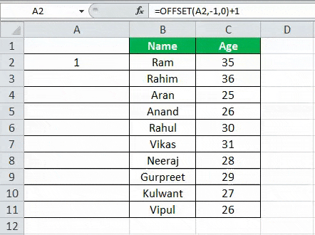
Using OFFSET Function
Dynamic numbering
Rows in Excel can also be numbered using the OFFSET function. It’s a slightly “off” the norm method but a method nonetheless and it requires you to start the column without a header; you’ll see why in a while.
The OFFSET function returns the value of the cell which is the given numbers of rows and columns from the specified cell. We will use this concept to then add 1 to each result to create serial numbering. Below is the demonstration with the formula:
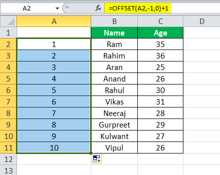
=OFFSET(B3,-1,0)+1
Now you’ll see why a blank column header was a prerequisite. Let’s understand the path in the formula. The cell specified is B3 itself. From there, OFFSET trails to -1 rows. This means B2. now in the third parameter of the formula, from B2 we need to shift to 0 columns which still leads to B2.
This means that using the OFFSET function, we will be referring to the previous cell in the same column. In the last bit of the formula, we have +1 which adds the number 1 to the value of B2. Since B2 is blank, 0+1 = 1. 1 is the outcome here. This is why we needed the header to be blank.
 15")
In the next instance, OFFSET will lead to B3 and add 1 to B3’s value. 1+1 = 2. That is how the rest of the rows will be numbered in succession.
Once you are done, you can copy and paste the values over themselves and add the column header if you so wish. The values are pasted back so that they are not formula-reliant and won’t cause errors.
 16")
Note: As long as the column header is absent, the results of this formula are dynamic. If you wish to add the column header, you will have to paste back the values or you can choose another method if want to retain the column header and the dynamic numbering.
Using SUBTOTAL Function
Dynamic numbering
And again, things were looking bright until you were hit with another requirement. You need to filter data but that would also filter the serial numbers. Now that’s a problem but not a problem we can’t work around. Enter SUBTOTAL function.
The SUBTOTAL function returns a subtotal in a dataset. While we will be using the COUNTA function via SUBTOTAL, SUBTOTAL will help to dynamically recalculate the row numbers as the data is filtered. Want to see how that works? We’ve got the formula to number rows with the SUBTOTAL function right ahead:
=SUBTOTAL(3,$C$3:C3)
The SUBTOTAL function presents a list of functions to choose from in the Formula AutoComplete. This parameter will determine what kind of subtotal you want to enter.
 17")
After selecting the function, the next input is the cell reference. As shown in the COUNTA function section above, we will enter $C$3:C3 as the range so that the count always begins from $C$3. As the formula is filled downward, the count will continue up until the target cell.
 18")
Now try filtering your data.
 19")
The row numbers will be recalculated with the filtered data serially numbered:
 20")
With the new serial number selected, we can note in the formula that the count for non-blank cells has started from $C$3 to C4 instead of C3. In this way, the count will begin from $C$3 and jump directly to the first filtered cell in the C column.
Creating Calculated Column in Excel Table
Dynamic numbering
Last but not least, let’s table it! An Excel table talks the talk and walks the walk and there are many convenient features it offers. The one helping us today is a calculated column; enter one formula and you’ll have numbered rows. Excel tables are known for being dynamic in their very nature and a calculated column also provides that ease. Nothing short of Excel magic. The complete tricks (read steps) to do this are as follows:
- Select any cell in the dataset. This will help Excel identify the range to create the Excel table.
- In the Home tab, go to the Styles section and click on the Format as a Table Select the table style from the menu or create your own.
 21")
- Now a small dialog box will appear confirming the identified range of the intended Excel table. Correct the range if required.
- If your table has headers, leave the My table has headers checkbox checked.
- Then click on the OK button to close the dialog box and apply the table.
 22")
- An Excel table will be created on the provided range:
 23")
- Now, enter this formula in any cell in the column where you want the numbers:
=ROW()-ROW(Table1[#Headers])
As a calculated column, when the formula is entered, all the rows will automatically be serially numbered:
 24")
And that’s your job done!
And that’s our tutorial done! The solutions may be numbered but so are the problems and today you saw how to tackle numbering rows in Excel in many different ways.
Filtering data and dealing with gaps in the data are two hitches you might face when numbering rows but today you’ve learned how to breeze through them. We’re up for making other hitches easy, breezy and we’re on it too so we’ll see you around another Excel trick!
While performing a simple numbering in Excel, we manually provide a cell number for the serial number; we can also do it automatically. To do auto numbering, we have two methods. First, we can fill the first two cells with the series of the number we want to be inserted and drag it down to the end of the table. The second method is to use the =ROW () formula which will give us the number, and then drag the formula similar to the end of the table.
For example, suppose you have a data set and want to start numbering them from 3 and step up by 4 until 40. First, you may select the cells containing the 3 and the 7. Then, click on the handle and drag to the other cells where you can see 40. You may then release and view that the numbers are filled in automatically.
You may also use the Excel ROW function = ROW() formula that returns the row number for reference. For example, ROW(A3) returns 3 as A3 is the third row in the spreadsheet. If not given any reference, ROW returns the cell’s row number, which consists of the formula.
Automatic Numbering in Excel
Numbering means giving serial numbers or numbers to a list of data. In Excel, no special button is provided that offers numbering for our data. As we already know, Excel does not provide a method, tool, or button to provide the sequential number to a list of data, which means we need to do it manually.
Table of contents
- Automatic Numbering in Excel
- How to Auto Number in Excel?
- Top 3 ways to get Auto Numbering in Excel
- #1 – Filling the Column with a Series of Numbers
- #2 – Use ROW() Function
- #3 – Using Offset() Function
- Things to Remember about Auto Numbering in Excel
- Auto Numbering in Excel Video
- Recommended Articles
How to Auto Number in Excel?
We must remember that our AutoFill functionAutoFill in excel can fill a range in a specific direction by using the fill handle.read more is always turned on to create auto numbering in Excel. By default, it is turned on. But in any case, if it is not enabled or mistakenly disabled “AutoFill,” here is how we can re-enable it.
Now we have checked that the “Autofill” is enabled. There are three methods for Excel auto-numbering:
- Fill a column with a series of numbers.
- Using the Row() function.
- Using the Offset() function.
The following are the steps for enabling fill handle and cell drag and drop: –
- In the “File” tab, go to “Options.”

- In the advanced section, check the “Enable fill handle and cell drag and drop” in Excel under the editing options.

Top 3 ways to get Auto Numbering in Excel
There are various ways to get automatic numbering in Excel.
You can download this Auto Numbering Excel Template here – Auto Numbering Excel Template
- Fill a column with a series of numbers.
- Use Row() function
- Use Offset() Function
Let us discuss all the above methods by examples.
#1 – Filling the Column with a Series of Numbers
We have the following data:
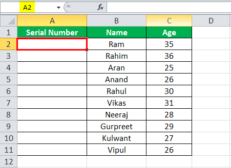
We will insert automatic numbers in Excel “column A” following the below steps:
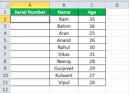
- We can select the cell we want to fill. In this example, we will choose cell A2.
- We will write the number we want to start with. Let it be 1, fill the next cell in the same column with another number, and let it be 2.
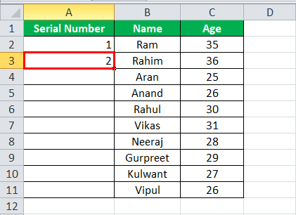
- To start a pattern, we have made the numbering 1 in cell A2 and 2 in cell A3. Next, we will select the starting values, i.e., cells A2 and A3.
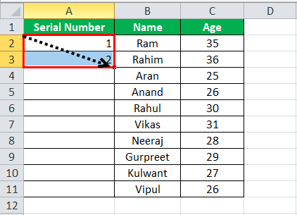
- The arrow shows the pointer (dot) in the selected cell. Then, click on it and drag it to the desired range, cell A11.
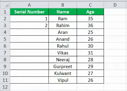
Now, we have sequential numbering for our data.
#2 – Use ROW() Function
We will use the same data to demonstrate the sequential numbering by the Row() functionThe row function in Excel is a worksheet function that displays the current row index number of the selected or target cell. The syntax to use this function is as follows: =ROW( Value ).read more.
- Below is our data:
- We select the specific cell where we want to start our automatic numbering in Excel (cell A2 in this case).
- We type ROW() in cell A2 and press “Enter.”
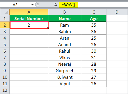
As a result, it gave us the numbering from number 2 since the Row function throws the number for the current row.
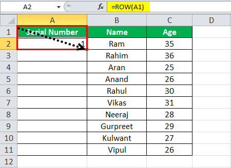
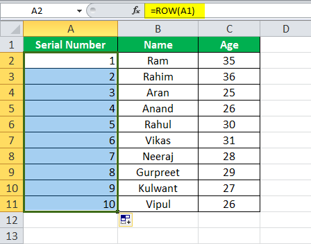
- To avoid the above situation, we can give the reference row to the Row function.

- Next, we click on the pointer or the dot in the selected cell and drag it to the desired range for the current scenario to cell A11.
- We have automatic numbering in Excel for the data using the Row() function.
#3 – Using Offset() Function
We can also achieve auto numbering in Excel using the Offset() functionThe OFFSET function in excel returns the value of a cell or a range (of adjacent cells) which is a particular number of rows and columns from the reference point. read more also.
Let us use the same data to demonstrate the Offset function. Below is the data:
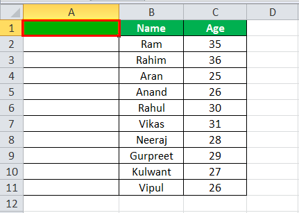
As we can see, we have removed the text written in cell A1 “Serial Number,” as the reference needs to be blank while using the Offset function.
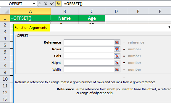
The above screenshot shows the function arguments used in the Offset function.
- In cell A2, we type offset(A2,-1,0)+1 for the automatic numbering in Excel.
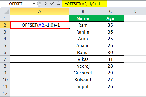
A2 is the current cell address, which is the reference.
- Press the “Enter” key. It will insert the first number.
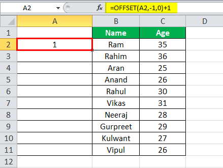
- Now, we select cell A2 and drag it down to cell A11.
- So, now we have sequential numbering using the Offset function.
Things to Remember about Auto Numbering in Excel
- Excel does not auto-provide auto-numbering.
- Do not forget to check for the enabled “AutoFill” option.
- While filling a column with a series of numbers, we must make a pattern. We can use the starting values as 2 or 4 to create even sequential numbering.
Auto Numbering in Excel Video
Recommended Articles
This article is a guide to Auto Numbering in Excel. Here, we discuss how to auto-number in Excel, along with Excel examples and downloadable Excel templates. You may also look at these useful Excel tools: –
- Excel VBA OFFSET
- Numbering in Excel
- WEEKDAY in ExcelThe WEEKDAY function in excel returns the day corresponding to a specified date. The date is supplied as an argument to this function. read more
- Equations in Excel
Bottom Line: Learn 4 different techniques for creating a list of numbers in Excel. These include both static and dynamic lists that change when items are added or deleted from the list.
Skill Level: Beginner
Watch the Tutorial
Download the Excel File
You can download the worksheet that I use in the video here:
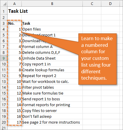
If you have a list of items in Excel and you’d like to insert a column that numbers the items, there are several ways to accomplish this. Let’s look at four of those ways.
1. Create a Static List Using Auto-Fill
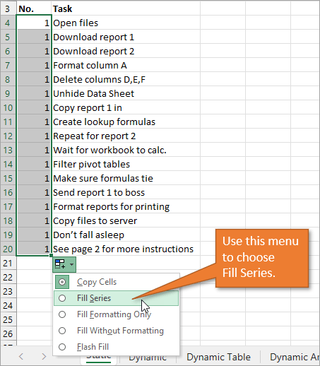
The first way to number a list is really easy. Start by filling in the first two numbers of your list, select those two numbers, and then hover over the bottom right corner of your selection until your cursor turns into a plus symbol. This is the fill handle.
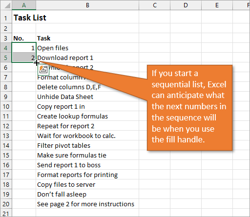
When you double-click on that fill handle (or drag it down to the end of your list), Excel will fill in the blanks with the next numbers in the sequence.
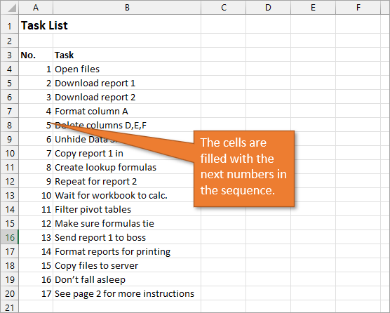
An alternate way to create this same numbered list is to type a 1 in the first cell and then double-click the fill handle. Because Excel doesn’t have a second number to identify a sequence or pattern, it will fill down the columns with 1s. But you will notice that a menu is available at the end of your column, and from that menu, you can select the option to Fill Series. This will change the 1s to a sequential list of numbers.
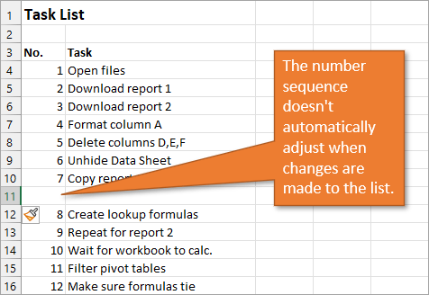
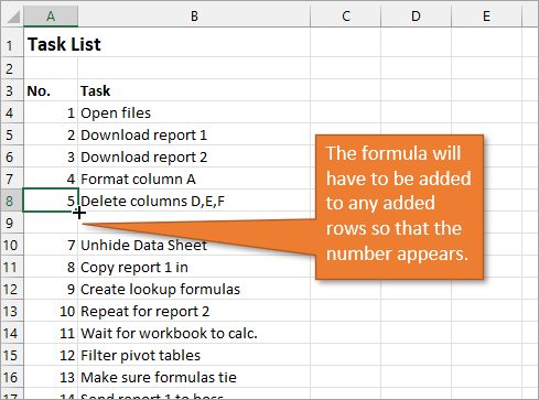
The numbered column we’ve created in both instances is static. This means it doesn’t change when you make additions or deletions to the corresponding list of items. For example, if I insert a new row in order to add another task, there is a break in the numbered column as well, and I would have to repeat the same steps to correct the list.
So, unless we want the numbers to always remain as they are, a better option would be to create a dynamic list.
2. Create a Dynamic List Using a Formula
We can use formulas to create a dynamic list where the numbers update when we add or delete rows from the list.
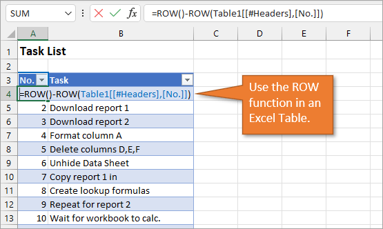
To use a formula for creating a dynamic number list, we can use the ROW function. The ROW function returns the row number of a cell. If we don’t specify a cell for ROW, it just returns the current row number of whatever is selected.
In our example, the first cell in our list doesn’t start on Row 1. It starts on Row 4. But we don’t want our list to start at 4; we want it to start at 1. To subtract the extra 3, our formula will include a minus sign and then the ROW function again, but this time pointed to the cell above our formula (which is in Row 3).
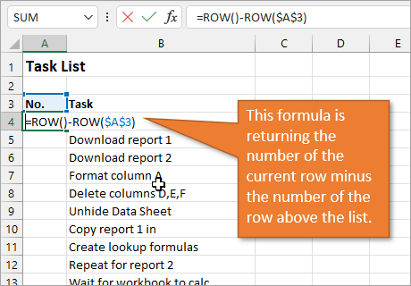
We use the absolute values (dollar signs) in our cell selection because we don’t want that number to change as we copy the formula down the list. In other words, we always want to subtract 3 from the row number to give us our list number.
When we copy down the formula, we have a numbered list that will adjust when we add or delete rows. However, when adding a row, we will have to copy the formula into the newly inserted cell.
This additional step of copying the formula into new rows can be avoided if we use Excel Tables.
3. Create a Dynamic List Using a Formula in an Excel Table
If we write the same formula but we use an Excel table, the only difference we will make in the formula is that we reference the column header instead of the absolute cell value.
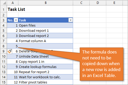
Because we are using an Excel Table, the formula automatically fills down to the other rows. When we add a row to the table, the formula will automatically populate in the new cell.
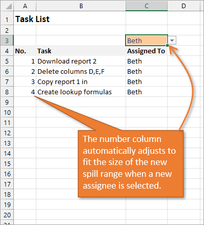
4. Create a Dynamic List Using Dynamic Array Formulas
Below, I have a table that is populated using Dynamic Array Formulas. The FILTER formula spills a range of results based on whatever name is selected in the orange cell.
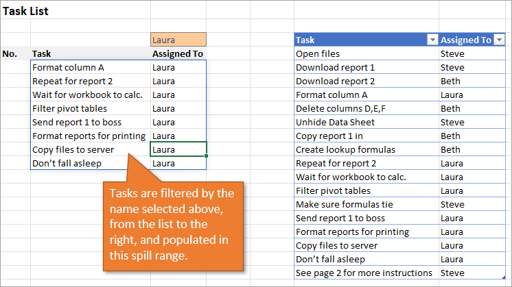
The Dynamic Array formula we will use is SEQUENCE. This will return a sequence for the number of rows we identify in the formula. To tell Excel how many rows there are, we will use the ROW function as the argument for sequence. The argument for ROW is just the spill range. The way to notate the spill range is to simply place a hashtag after the name of the first cell in the range. So our formula looks like this:
=SEQUENCE(ROWS(B5#))
Once we complete our formula and hit Enter, the list will be numbered.
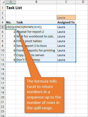
With this formula in place, if the size of the range changes when a new name is selected, the numbered column for the list will automatically adjust as well.
Bonus Tip: Formatting Your Numbered List
If you want to add periods or other punctuation to your numbered list:
- Select the entire list and right-click to choose Format Cells. Or use the keyboard shortcut Ctrl + 1.
- Choose the Custom option on the Number tab.
- Then in the Type field, type in the number 0 with whatever punctuation you would like to surround your number.
Here, I’ve just added a period.
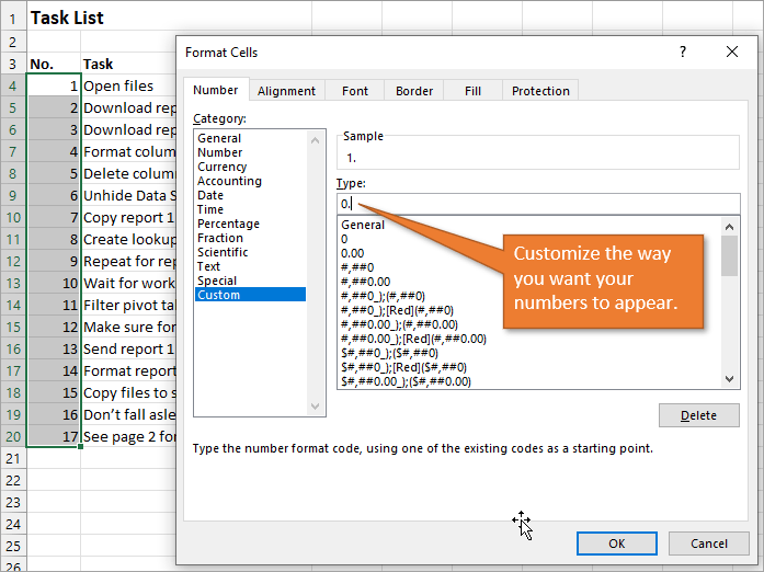
When you hit OK, you will have formatted the entire selection.
Related Posts
Here are a few similar posts that may interest you.
- Excel Tables Tutorial Video – Beginners Guide for Windows & Mac
- New Excel Features: Dynamic Array Formulas & Spill Ranges
- How to Prevent Excel from Freezing or Taking A Long Time when Deleting Rows
Conclusion
I hope these four ways to create ordered lists are helpful for you. If you have questions or feedback, I would love to hear them in the comments. Have a great week!