
Содержание
- Способы нумерации
- Способ 1: маркер заполнения
- Способ 2: нумерация с помощью кнопки «Заполнить» на ленте
- Способ 3: функция СТОЛБЕЦ
- Вопросы и ответы

При работе с таблицами довольно часто требуется произвести нумерацию столбцов. Конечно, это можно сделать вручную, отдельно вбивая номер для каждого столбца с клавиатуры. Если же в таблице очень много колонок, это займет значительное количество времени. В Экселе есть специальные инструменты, позволяющие провести нумерацию быстро. Давайте разберемся, как они работают.
Способы нумерации
В Excel существует целый ряд вариантов автоматической нумерации столбцов. Одни из них довольно просты и понятны, другие – более сложные для восприятия. Давайте подробно остановимся на каждом из них, чтобы сделать вывод, какой вариант использовать продуктивнее в конкретном случае.
Способ 1: маркер заполнения
Самым популярным способом автоматической нумерации столбцов, безусловно, является использования маркера заполнения.
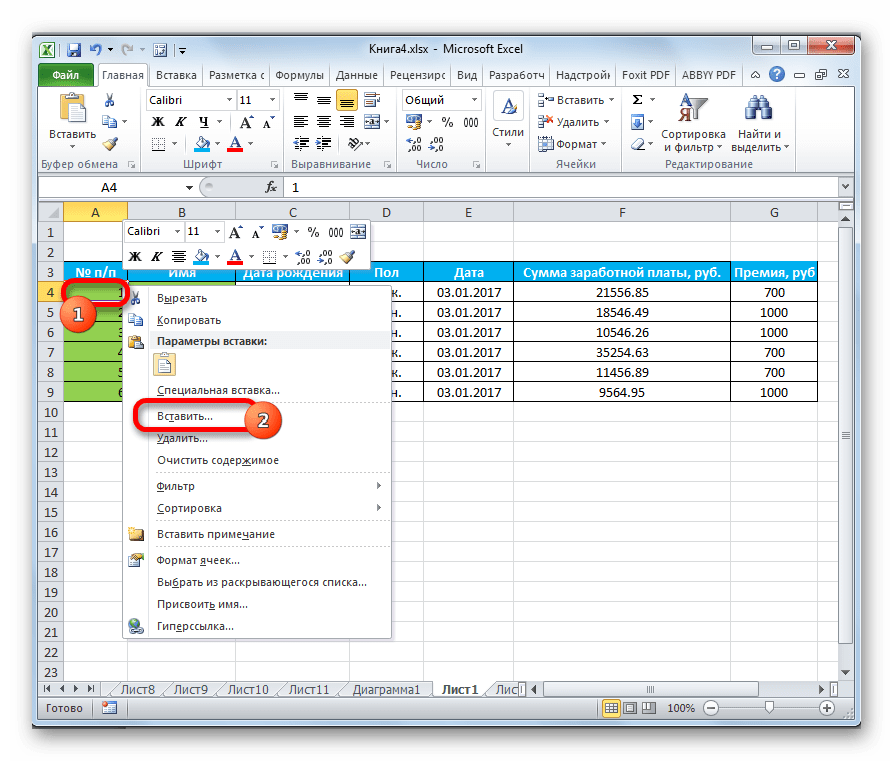
- Открываем таблицу. Добавляем в неё строку, в которой будет размещаться нумерация колонок. Для этого, выделяем любую ячейку строки, которая будет находиться сразу под нумерацией, кликаем правой кнопкой мыши, тем самым вызвав контекстное меню. В этом списке выбираем пункт «Вставить…».
- Открывается небольшое окошко вставки. Переводим переключатель в позицию «Добавить строку». Жмем на кнопку «OK».
- В первую ячейку добавленной строки ставим цифру «1». Затем наводим курсор на нижний правый угол этой ячейки. Курсор превращается в крестик. Именно он называется маркером заполнения. Одновременно зажимаем левую кнопку мыши и клавишу Ctrl на клавиатуре. Тянем маркер заполнения вправо до конца таблицы.
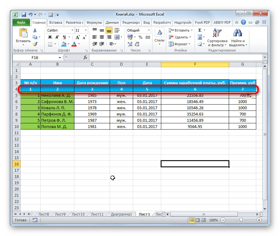
- Как видим, нужная нам строка заполнена номерами по порядку. То есть, была проведена нумерация столбцов.


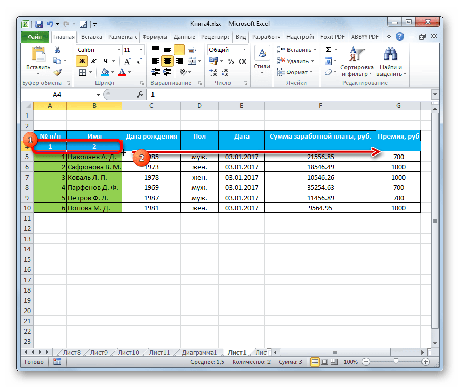
Можно также поступить несколько иным образом. Заполняем первые две ячейки добавленной строки цифрами «1» и «2». Выделяем обе ячейки. Устанавливаем курсор в нижний правый угол самой правой из них. С зажатой кнопкой мыши перетягиваем маркер заполнения к концу таблицы, но на этот раз на клавишу Ctrl нажимать не нужно. Результат будет аналогичным.
Хотя первый вариант данного способа кажется более простым, но, тем не менее, многие пользователи предпочитают пользоваться вторым.
Существует ещё один вариант использования маркера заполнения.
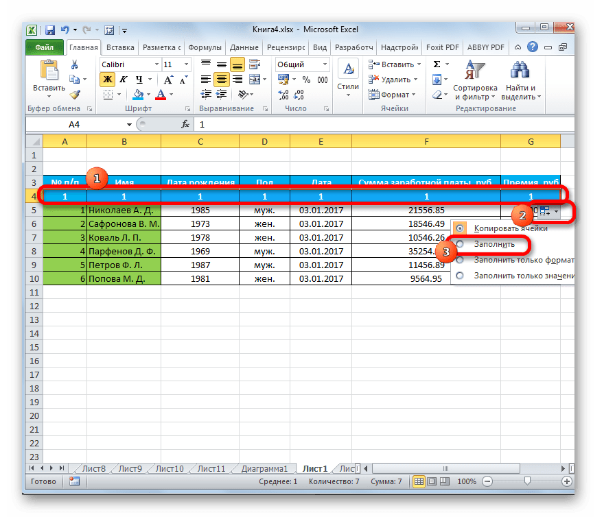
- В первой ячейке пишем цифру «1». С помощью маркера копируем содержимое вправо. При этом опять кнопку Ctrl зажимать не нужно.
- После того, как выполнено копирование, мы видим, что вся строка заполнена цифрой «1». Но нам нужна нумерация по порядку. Кликаем на пиктограмму, которая появилась около самой последней заполненной ячейки. Появляется список действий. Производим установку переключателя в позицию «Заполнить».
После этого все ячейки выделенного диапазона будет заполнены числами по порядку.

Урок: Как сделать автозаполнение в Excel
Способ 2: нумерация с помощью кнопки «Заполнить» на ленте
Ещё один способ нумерации колонок в Microsoft Excel подразумевает использование кнопки «Заполнить» на ленте.
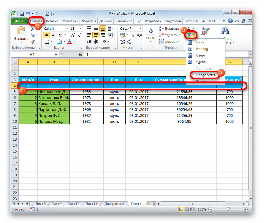
- После того, как добавлена строка для нумерации столбцов, вписываем в первую ячейку цифру «1». Выделяем всю строку таблицы. Находясь во вкладке «Главная», на ленте жмем кнопку «Заполнить», которая расположена в блоке инструментов «Редактирование». Появляется выпадающее меню. В нём выбираем пункт «Прогрессия…».
- Открывается окно настроек прогрессии. Все параметры там уже должны быть настроены автоматически так, как нам нужно. Тем не менее, не лишним будет проверить их состояние. В блоке «Расположение» переключатель должен быть установлен в позицию «По строкам». В параметре «Тип» должно быть выбрано значение «Арифметическая». Автоматическое определение шага должно быть отключено. То есть, не нужно, чтобы около соответствующего наименования параметра стояла галочка. В поле «Шаг» проверьте, чтобы стояла цифра «1». Поле «Предельное значение» должно быть пустым. Если какой-то параметр не совпадает с позициями, озвученными выше, то выполните настройку согласно рекомендациям. После того, как вы удостоверились, что все параметры заполнены верно, жмите на кнопку «OK».
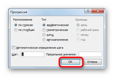
Вслед за этим столбцы таблицы будут пронумерованы по порядку.
Можно даже не выделять всю строку, а просто поставить в первую ячейку цифру «1». Затем вызвать окно настройки прогрессии тем же способом, который был описан выше. Все параметры должны совпадать с теми, о которых мы говорили ранее, кроме поля «Предельное значение». В нём следует поставить число столбцов в таблице. Затем жмите на кнопку «OK».
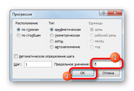
Заполнение будет выполнено. Последний вариант хорош для таблиц с очень большим количеством колонок, так как при его применении курсор никуда тащить не нужно.
Способ 3: функция СТОЛБЕЦ
Можно также пронумеровать столбцы с помощью специальной функции, которая так и называется СТОЛБЕЦ.
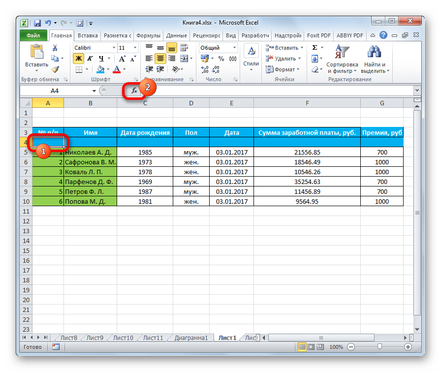
- Выделяем ячейку, в которой должен находиться номер «1» в нумерации колонок. Кликаем по кнопке «Вставить функцию», размещенную слева от строки формул.
- Открывается Мастер функций. В нём размещен перечень различных функций Excel. Ищем наименование «СТОЛБЕЦ», выделяем его и жмем на кнопку «OK».
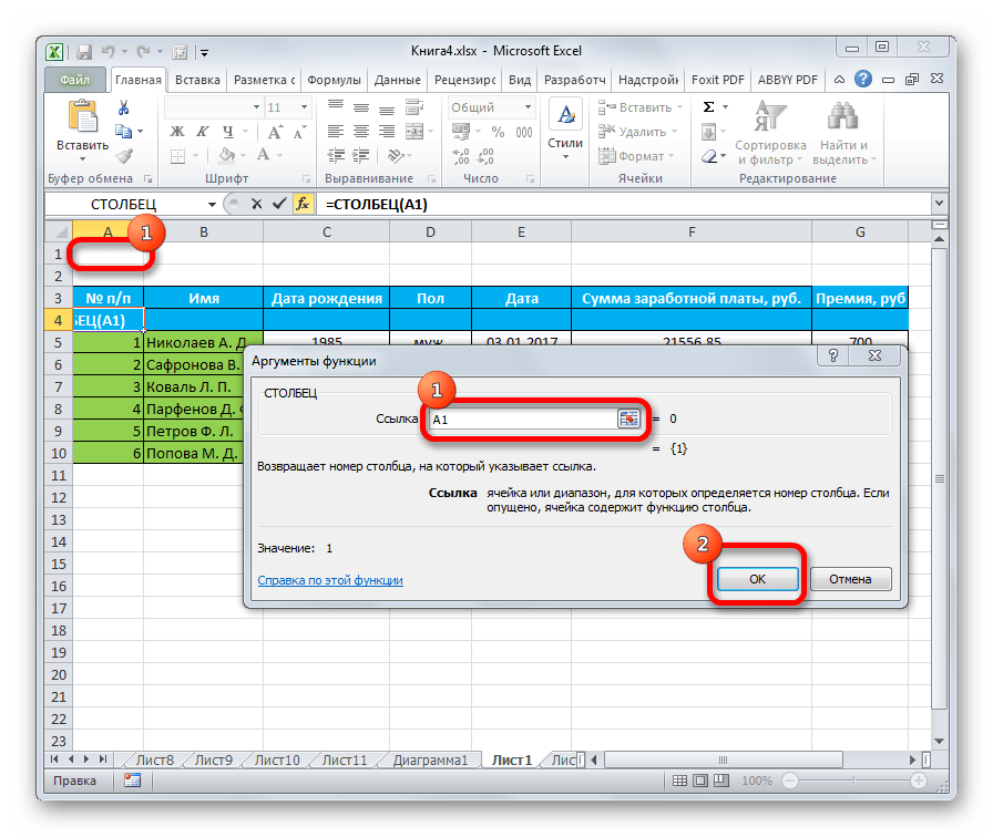
- Открывается окно аргументов функции. В поле «Ссылка» нужно указать ссылку на любую ячейку первого столбца листа. На этот момент крайне важно обратить внимание, особенно, если первая колонка таблицы не является первым столбцом листа. Адрес ссылки можно прописать вручную. Но намного проще это сделать установив курсор в поле «Ссылка», а затем кликнув по нужной ячейке. Как видим, после этого, её координаты отображаются в поле. Жмем на кнопку «OK».
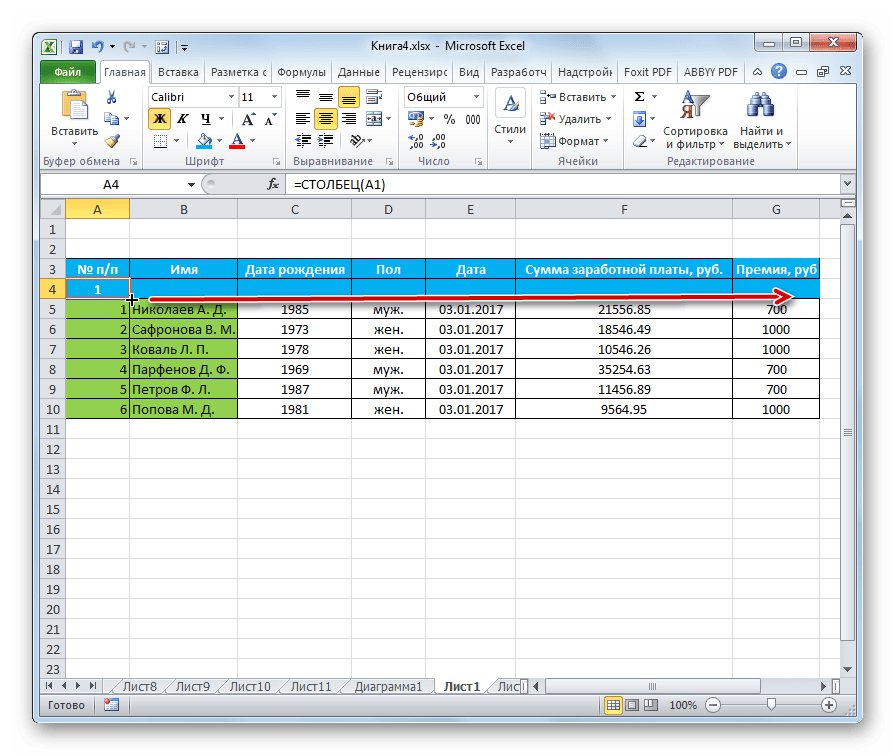
- После этих действий в выделенной ячейке появляется цифра «1». Для того, чтобы пронумеровать все столбцы, становимся в её нижний правый угол и вызываем маркер заполнения. Так же, как и в предыдущие разы протаскиваем его вправо к концу таблицы. Зажимать клавишу Ctrl не нужно, нажимаем только правую кнопку мыши.

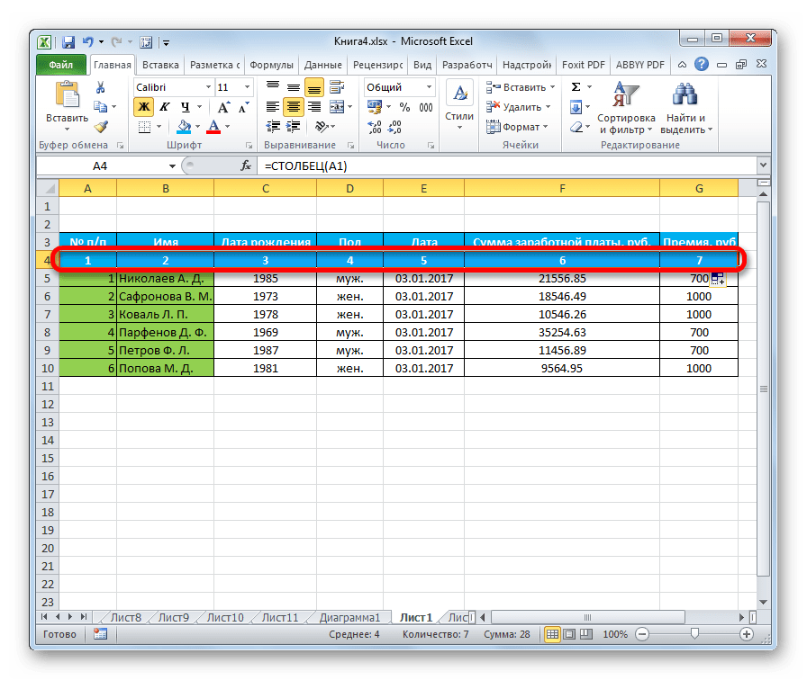
После выполнения всех вышеуказанных действий все колонки таблицы будут пронумерованы по порядку.
Урок: Мастер функций в Excel
Как видим, произвести нумерацию столбцов в Экселе можно несколькими способами. Наиболее популярный из них – использование маркера заполнения. В слишком широких таблицах есть смысл использовать кнопку «Заполнить» с переходом в настройки прогрессии. Данный способ не предполагает манипуляции курсором через всю плоскость листа. Кроме того, существует специализированная функция СТОЛБЕЦ. Но из-за сложности использования и заумности данный вариант не является популярным даже у продвинутых пользователей. Да и времени данная процедура занимает больше, чем обычное использование маркера заполнения.
Еще статьи по данной теме:
Помогла ли Вам статья?
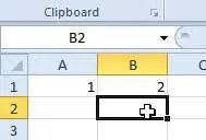
Auto number a column by AutoFill function Type 1 into a cell that you want to start the numbering, then drag the autofill handle at the right-down corner of the cell to the cells you want to number, and click the fill options to expand the option, and check Fill Series, then the cells are numbered.
Contents
- 1 How do I number multiple columns in Excel?
- 2 How do you label Excel columns with numbers?
- 3 How do you create a number sequence in Excel without dragging?
- 4 How do I change a number to a percent in Excel?
- 5 How do I show columns and row numbers in Excel?
- 6 How do I add a numbered column in numbers?
- 7 How do I make a numbered list in numbers?
- 8 How do I apply a formula to an entire column in numbers?
- 9 How do I change the order of columns in Excel?
- 10 How do you auto fill columns in Excel?
- 11 How do you make a number into a percent?
- 12 How do you change a number back to a percentage?
- 13 How do you change a number into percentage?
- 14 How do you show columns in Excel?
- 15 Why can’t I see Row numbers in Excel?
- 16 How are columns labeled in an Excel worksheet?
- 17 How do I add numbers in columns in pages?
- 18 What is a numbered list?
- 19 How do I create a list style in pages?
- 20 How do you format a list?
Fill a column with a series of numbers
- Select the first cell in the range that you want to fill.
- Type the starting value for the series.
- Type a value in the next cell to establish a pattern.
- Select the cells that contain the starting values.
- Drag the fill handle.
How do you label Excel columns with numbers?
To change the column headings to letters, select the File tab in the toolbar at the top of the screen and then click on Options at the bottom of the menu. When the Excel Options window appears, click on the Formulas option on the left. Then uncheck the option called “R1C1 reference style” and click on the OK button.
How do you create a number sequence in Excel without dragging?
The regular way of doing this is: Enter 1 in cell A1. Enter 2 in cell A2. Select both the cells and drag it down using the fill handle.
Quickly Fill Numbers in Cells without Dragging
- Enter 1 in cell A1.
- Go to Home –> Editing –> Fill –> Series.
- In the Series dialogue box, make the following selections:
- Click OK.
How do I change a number to a percent in Excel?
How to Apply the Percent Number Format in Excel 2010
- Select the cells containing the numbers you want to format.
- On the Home tab, click the Number dialog box launcher in the bottom-right corner of the Number group.
- In the Category list, select Percentage.
- Specify the number of decimal places.
- Click OK.
How do I show columns and row numbers in Excel?
On the Ribbon, click the Page Layout tab. In the Sheet Options group, under Headings, select the Print check box. , and then under Print, select the Row and column headings check box .
How do I add a numbered column in numbers?
Click the table. in the top-right corner of the table to add a column, or drag it to add or delete multiple columns. You can delete a row or column only if all of its cells are empty.
How do I make a numbered list in numbers?
Select the list items with the numbering or lettering you want to change. In the Format sidebar, click the Text tab, then click the Style button near the top of the sidebar. Click the disclosure arrow next to Bullets & Lists, then click the pop-up menu below Bullets & Lists and choose Numbers.
How do I apply a formula to an entire column in numbers?
Select that cell. You will see a small circle in the bottom-right corner of the cell. Click and drag that down and all cells below will auto-fill with the number 50 (or a formula if you have that in a cell). Works in a fill-right direction too.
How do I change the order of columns in Excel?
To quickly move columns in Excel without overwriting existing data, press and hold the shift key on your keyboard.
- First, select a column.
- Hover over the border of the selection.
- Press and hold the Shift key on your keyboard.
- Click and hold the left mouse button.
- Move the column to the new position.
How do you auto fill columns in Excel?
Click and hold the left mouse button, and drag the plus sign over the cells you want to fill. And the series is filled in for you automatically using the AutoFill feature. Or, say you have information in Excel that isn’t formatted the way you need it to be, such as this list of names.
How do you make a number into a percent?
To turn a percent into an integer or decimal number, simply divide by 100. That is the same as moving the decimal point two places to the left.
How do you change a number back to a percentage?
Step 1) Get the percentage of the original number. If the percentage is an increase then add it to 100, if it is a decrease then subtract it from 100. Step 2) Divide the percentage by 100 to convert it to a decimal. Step 3) Divide the final number by the decimal to get back to the original number.
How do you change a number into percentage?
Percentage Change | Increase and Decrease
- First: work out the difference (increase) between the two numbers you are comparing.
- Increase = New Number – Original Number.
- Then: divide the increase by the original number and multiply the answer by 100.
- % increase = Increase ÷ Original Number × 100.
How do you show columns in Excel?
How to show hidden columns that you select
- Select the columns to the left and right of the column you want to unhide. For example, to show hidden column B, select columns A and C.
- Go to the Home tab > Cells group, and click Format > Hide & Unhide > Unhide columns.
Why can’t I see Row numbers in Excel?
Step 1 – Click on “View” Tab on Excel Ribbon. Step 3 – Uncheck “Headings” checkbox to hide Excel worksheet Row and Column headings. Check “Headings” checkbox to show missing hidden Excel worksheet Row and Column headings, as explained in below image.
How are columns labeled in an Excel worksheet?
How are columns and rows labeled? In all spreadsheet programs including Microsoft Excel, rows are labeled using numbers (e.g., 1 to 1,048,576). All columns are labeled with letters starting with the letter A and then incrementing by a letter after the final letter Z.
How do I add numbers in columns in pages?
Inserting columns in Pages
- 1) Open your document or create a new one in Pages.
- 2) Click the Format button on the top right to open the formatting sidebar.
- 3) Click the Layout button and you should see the Columns settings right below it.
- 4) Use the arrows or pop in a number for the number of columns you want to insert.
What is a numbered list?
Numbered-list meaning. Filters. A list whose items are numbered, with various styles including Arabic numerals and Roman numerals. noun. 5.
How do I create a list style in pages?
In the Format sidebar, click the Style button near the top. If the text is in a text box, table, or shape, first click the Text tab at the top of the sidebar, then click the Style button. Click the pop-up menu next to Bullets & Lists, then choose a list style.
How do you format a list?
Format for Lists
- Use a colon to introduce the list items only if a complete sentence precedes the list.
- Use both opening and closing parentheses on the list item numbers or letters: (a) item, (b) item, etc.
- Use either regular Arabic numbers or lowercase letters within the parentheses, but use them consistently.
Excel for Microsoft 365 Excel for Microsoft 365 for Mac Excel for the web Excel 2021 Excel 2021 for Mac Excel 2019 Excel 2019 for Mac Excel 2016 Excel 2016 for Mac Excel 2013 More…Less
If you need a quick way to count rows that contain data, select all the cells in the first column of that data (it may not be column A). Just click the column header. The status bar, in the lower-right corner of your Excel window, will tell you the row count.
Do the same thing to count columns, but this time click the row selector at the left end of the row.
The status bar then displays a count, something like this:

If you select an entire row or column, Excel counts just the cells that contain data. If you select a block of cells, it counts the number of cells you selected. If the row or column you select contains only one cell with data, the status bar stays blank.
Notes:
-
If you need to count the characters in cells, see Count characters in cells.
-
If you want to know how many cells have data, see Use COUNTA to count cells that aren’t blank.
-
You can control the messages that appear in the status bar by right-clicking the status bar and clicking the item you want to see or remove. For more information, see Excel status bar options.
Need more help?
You can always ask an expert in the Excel Tech Community or get support in the Answers community.
Need more help?
How to Get a Column Number in Excel: Easy Tutorial (2023)
An Excel sheet is two-dimensional – it has rows and columns. By default, row headers in Excel are numbers, and column headers are alphabets.
As the data in your Excel sheet starts to grow in width, the number of columns grows. And this might make it difficult for you to track down a column by its number.
The article below explains different methods of how you can get column numbers in Excel. Also, it focuses on how column numbers might help you in your Excel jobs.
So stay tuned till the end! 😀
Practice the examples shown in the article below by downloading the sample workbook here.
How to get column number with the COLUMN function
If you have never before heard of the COLUMN function, it’s alright. Most Excel users have not.
The COLUMN function of Excel is designed to return the number of a column in Excel.
To find the column numbers for different columns in Excel, see the example below.

1. Write the COLUMN formula.
=COLUMN()
And this is it!
The COLUMN function has just one argument – the reference argument. Interestingly, this argument is also optional.
If omitted, Excel deems it equal to the Cell reference where the formula is written.

We had omitted the argument, so Excel set it equal to Cell B2. Column B comes second in the sequence, so Excel returned ‘2’ as the Column number.
Let’s see this the other way around.
2. Set the reference argument to AAX10.


This time Excel returns column number 726. This means Column AAX is the 726th Column of Excel.
How many columns are there in an Excel Sheet?
The last column of an Excel worksheet is Column XFD. So how many columns are there in a single worksheet?
Let’s do it quickly!
- Press Ctrl + the right arrow button ➡️ to fast forward to the last column of Excel.
- Write the Column formula.
=COLUMN()

16384 Excel Columns to each worksheet.
Let’s double-check the same from Google! 😆

Examples of uses for the COLUMN function
Why would anyone want to use the COLUMN function? The examples below tell why.
Example 1:
The image below shows the grades of a few students (to the left).

To the right side, we want to fetch out the grades for Henry. Easy solution = VLOOKUP.
1. Write the VLOOKUP function as follows.
= VLOOKUP (E1,

The lookup_value is referred to as Cell E1 because it contains the name of the student to look the result for.
2. Refer to the table array where the lookup and the return values are.
= VLOOKUP (E1, A1:B4,

3. For the col_index num argument, nest in the COLUMN function as follows:
= VLOOKUP (F1, A1:B4, COLUMN(B1))
The col_index num argument refers to the column from where the value is to be returned.
And this has to be the number of the column starting from the first column of the table_array.

We want the Grades of Henry to be returned. Grades are listed in column B, so we have referred to Cell B1 (any cell from Column B).

Instead of manually counting the columns, let the COLUMN function do the job.
The VLOOKUP function needs the column number starting from the table array. If the table array starts from any column other than the first column, the above function might not work.
For example, what if the table array above started from Column B and not A?

1. Write the VLOOKUP function as above, and it’d fail to function.
=VLOOKUP (G2, B1:C4, (COLUMN (C1))
It will take the col_index num argument as 3 (Column number of Column C).
Whereas, our table range has only two columns.

2. Deal with such a situation by changing the COLUMN function as follows.
= COLUMN(C1) – COLUMN(A1)
Subtract the number of the column before the table array (Column A) from the return value column (Column C).
3. Rewrite the VLOOKUP function as below.
= VLOOKUP (G1, B1:C4, COLUMN(C1) – COLUMN(A1))
Here are the results!

Example 2:
The COLUMN function is not only meant to find the number of a single column. You can also use it to find the number of multiple columns at once.
The data below shows the monthly utility bill of a household.

To find the accumulated utility bill for each month, let’s apply the COLUMN function.
1. Write the COLUMN function as follows.
=COLUMN(A2:F2)

The range A2:F2 tells the number of months for which we need the accumulated bill.

2. Multiply it with the particular cell of the monthly bill.
= H3 * COLUMN(A2:F2)
The cell reference is set to H3 as it contains the monthly bill.


It only takes a single click for Excel to compute the bills for all the months.
When the reference argument of the column function is defined as a range, the output is an array.
Caution! The SPILL Error:
If the cells of the array are not vacant before the array function operates, Excel gives the #SPILL! Error.

Show column number instead of letter
Only if Excel labeled both the rows and columns with numbers and not alphabets – things would have been much easier!
If you think like that, let’s do it for you.
To change the column letter to numbers in Excel, continue reading.
1. Go to File > Options
2. This opens up the Excel options dialog box.

3. Go to Formulas.
4. Under the tab, ‘Working with Formulas’, check the box R1C1 Reference Style.

And swish! Magic. The reference style of columns has changed. 😉

Your Excel worksheet looks all new with a new reference style! Both columns and rows are labeled by numbers.
The R1C1 style reference indicates the Row number and Column number. Accordingly, the cell references will automatically change.
For example, the traditional Cell reference C5 has now become R5C3 (Row number 5 and Column number 3).

This way, you can easily track down the number of columns.
That’s it – Now what?
By now, we have learned to find the column number in Excel through the COLUMN formula, to nest the COLUMN formula in VLOOKUP, and also to change the Column reference style in Excel.
But that’s all about basic Excel. To become an Excel pro you must master the VLOOKUP, SUMIF, and IF functions.
Where can you learn them? Click here to sign up for my free 30-minute email course that will help you master these functions (and more!).
Other relevant resources:
Finding the column number for a specific column or a group of columns can simplify your Excel jobs.
We suggest you also take a quick look into some shortcuts for adding, moving, splitting, clustering, and comparing columns. Once you have learned these shortcuts and tips, you’ll feel no less than an Excel whizz.
Kasper Langmann2023-01-19T12:23:31+00:00
Page load link
When you need to assign consecutive numbers to rows or columns in Microsoft Excel 2010, it can be very frustrating to do it manually. Aside from the amount of time that it can take, it is very easy to make mistakes, forcing you to go back and re-do your work. Fortunately there is a feature in Excel 2010 that allows you to enter two numbers to start a sequence, then expand that sequence across as many cells as you need. We have previously written about how to automatically number rows in Excel 2010, and the method for numbering columns in Excel 2010 is very similar.
Automatic Column Numbering in Excel 2010
This tutorial is going to assume that you want to fill in a series of cells at the top of your columns (in the first row) with numbers that increase by one as they progress from left to right. I am going to be starting with “1” and going up from there, but you can use any two numbers and Excel will continue the pattern that exists between those numbers for however many cells you select. For example, you could enter “2” and “4” into the first two cells of your sequence, and Excel would continue numbering the rest of your cells with increasing even numbers.
Step 1: Open your spreadsheet in Excel 2010.
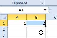
Step 2: Type the first two numbers of your sequence into the first two cells into which you want your automatic numbering to start.
Step 3: Use your mouse to highlight the two cells containing the values that you just entered.
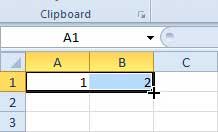
Step 4: Position your mouse on the bottom-right corner of the rightmost cell so that your cursor changes to the shape in the image below.
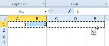
Step 5: Click and hold the left mouse button down and drag it to the right to select the cells that you want to automatically number. Note that the number under your cursor will display the value that will be entered into the currently selected cell.
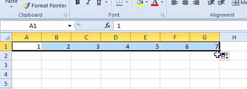
Step 6: Release the mouse button to finish your automatic numbering.
Do you have a Netflix, Hulu, Amazon Prime or HBO Go account, and you’re looking for a cheap and easy way to watch that streaming video on your TV? Check out the Roku LT, one of the most popular solutions available on the market.
If you are printing out large documents, page numbers can be very helpful. Learn how to insert page numbers at the bottom of the page in Excel 2010.

Matthew Burleigh has been writing tech tutorials since 2008. His writing has appeared on dozens of different websites and been read over 50 million times.
After receiving his Bachelor’s and Master’s degrees in Computer Science he spent several years working in IT management for small businesses. However, he now works full time writing content online and creating websites.
His main writing topics include iPhones, Microsoft Office, Google Apps, Android, and Photoshop, but he has also written about many other tech topics as well.
Read his full bio here.