
A Data Model allows you to integrate data from multiple tables, effectively building a relational data source inside an Excel workbook. Within Excel, Data Models are used transparently, providing tabular data used in PivotTables and PivotCharts. A Data Model is visualized as a collection of tables in a Field List, and most of the time, you’ll never even know it’s there.
Before you can start working with the Data Model, you need to get some data. For that we’ll use the Get & Transform (Power Query) experience, so you might want to take a step back and watch a video, or follow our learning guide on Get & Transform and Power Pivot.
Where is Power Pivot?
-
Excel 2016 & Excel for Microsoft 365 — Power Pivot is included in the Ribbon.
-
Excel 2013 — Power Pivot is part of the Office Professional Plus edition of Excel 2013, but is not enabled by default. Learn more about starting the Power Pivot add-in for Excel 2013.
-
Excel 2010 — Download the Power Pivot add-in, then install the Power Pivot add-in.
Where is Get & Transform (Power Query)?
-
Excel 2016 & Excel for Microsoft 365 — Get & Transform (Power Query) has been integrated with Excel on the Data tab.
-
Excel 2013 — Power Query is an add-in that’s included with Excel, but needs to be activated. Go to File > Options > Add-Ins, then in the Manage drop-down at the bottom of the pane, select COM Add-Ins > Go. Check Microsoft Power Query for Excel, then OK to activate it. A Power Query tab will be added to the ribbon.
-
Excel 2010 — Download and install the Power Query add-in.. Once activated, a Power Query tab will be added to the ribbon.
Getting started
First, you need to get some data.
-
In Excel 2016, and Excel for Microsoft 365, use Data > Get & Transform Data > Get Data to import data from any number of external data sources, such as a text file, Excel workbook, website, Microsoft Access, SQL Server, or another relational database that contains multiple related tables.
In Excel 2013 and 2010, go to Power Query > Get External Data, and select your data source.
-
Excel prompts you to select a table. If you want to get multiple tables from the same data source, check the Enable selection of multiple tables option. When you select multiple tables, Excel automatically creates a Data Model for you.

-
Select one or more tables, then click Load.
If you need to edit the source data, you can choose the Edit option. For more details see: Introduction to the Query Editor (Power Query).

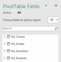
You now have a Data Model that contains all of the tables you imported, and they will be displayed in the PivotTable Field List.
Notes:
-
Models are created implicitly when you import two or more tables simultaneously in Excel.
-
Models are created explicitly when you use the Power Pivot add-in to import data. In the add-in, the model is represented in a tabbed layout similar to Excel, where each tab contains tabular data. See Get data using the Power Pivot add-into learn the basics of data import using a SQL Server database.
-
A model can contain a single table. To create a model based on just one table, select the table and click Add to Data Model in Power Pivot. You might do this if you want to use Power Pivot features, such as filtered datasets, calculated columns, calculated fields, KPIs, and hierarchies.
-
Table relationships can be created automatically if you import related tables that have primary and foreign key relationships. Excel can usually use the imported relationship information as the basis for table relationships in the Data Model.
-
For tips on how to reduce the size of a data model, see Create a memory-efficient Data Model using Excel and Power Pivot.
-
For further exploration, see Tutorial: Import Data into Excel, and Create a Data Model.
Create Relationships between your tables
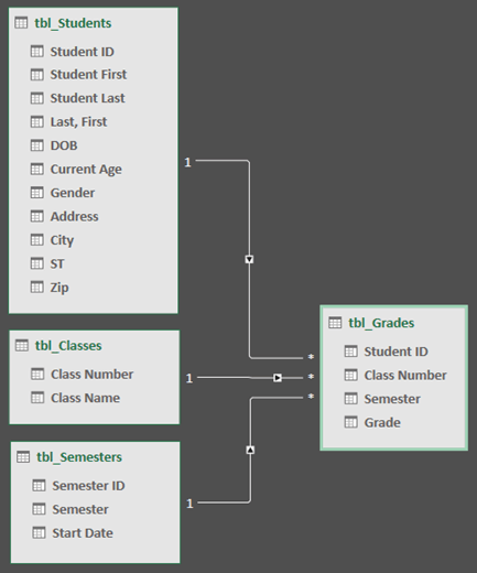
The next step is to create relationships between your tables, so you can pull data from any of them. Each table needs to have a primary key, or unique field identifier, like Student ID, or Class number. The easiest way is to drag and drop those fields to connect them in Power Pivot’s Diagram View.
-
Go to Power Pivot > Manage.
-
On the Home tab, select Diagram View.
-
All of your imported tables will be displayed, and you might want to take some time to resize them depending on how many fields each one has.
-
Next, drag the primary key field from one table to the next. The following example is the Diagram View of our student tables:
We’ve created the following links:
-
tbl_Students | Student ID > tbl_Grades | Student ID
In other words, drag the Student ID field from the Students table to the Student ID field in the Grades table.
-
tbl_Semesters | Semester ID > tbl_Grades | Semester
-
tbl_Classes | Class Number > tbl_Grades | Class Number
Notes:
-
Field names don’t need to be the same in order to create a relationship, but they do need to be the same data type.
-
The connectors in the Diagram View have a «1» on one side, and an «*» on the other. This means that there is a one-to-many relationship between the tables, and that determines how the data is used in your PivotTables. See: Relationships between tables in a Data Model to learn more.
-
The connectors only indicate that there is a relationship between tables. They won’t actually show you which fields are linked to each other. To see the links, go to Power Pivot > Manage > Design > Relationships > Manage Relationships. In Excel, you can go to Data > Relationships.
-
Use a Data Model to create a PivotTable or PivotChart
An Excel workbook can contain only one Data Model, but that model can contain multiple tables which can be used repeatedly throughout the workbook. You can add more tables to an existing Data Model at any time.
-
In Power Pivot, go to Manage.
-
On the Home tab, select PivotTable.
-
Select where you want the PivotTable to be placed: a new worksheet, or the current location.
-
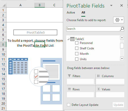
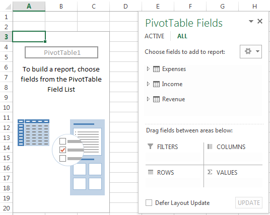
Click OK, and Excel will add an empty PivotTable with the Field List pane displayed on the right.
Next, create a PivotTable, or create a Pivot Chart. If you’ve already created relationships between the tables, you can use any of their fields in the PivotTable. We’ve already created relationships in the Student Data Model sample workbook.
Add existing, unrelated data to a Data Model
Suppose you’ve imported or copied lots of data that you want to use in a model, but haven’t added it to the Data Model. Pushing new data into a model is easier than you think.
-
Start by selecting any cell within the data that you want to add to the model. It can be any range of data, but data formatted as an Excel table is best.
-
Use one of these approaches to add your data:
-
Click Power Pivot > Add to Data Model.
-
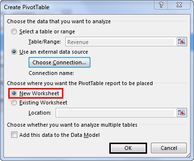
Click Insert > PivotTable, and then check Add this data to the Data Model in the Create PivotTable dialog box.
The range or table is now added to the model as a linked table. To learn more about working with linked tables in a model, see Add Data by Using Excel Linked Tables in Power Pivot.
Adding data to a Power Pivot table
In Power Pivot, you cannot add a row to a table by directly typing in a new row like you can in an Excel worksheet. But you can add rows by copying and pasting, or updating the source data and refreshing the Power Pivot model.
Need more help?
You can always ask an expert in the Excel Tech Community or get support in the Answers community.
See Also
Get & Transform and Power Pivot learning guides
Introduction to the Query Editor (Power Query)
Create a memory-efficient Data Model using Excel and Power Pivot
Tutorial: Import Data into Excel, and Create a Data Model
Find out which data sources are used in a workbook data model
Relationships between tables in a Data Model
It can be any range of data, but data formatted as an Excel table is best. Use one of these approaches to add your data: Click Power Pivot > Add to Data Model. Click Insert > PivotTable, and then check Add this data to the Data Model in the Create PivotTable dialog box.
Contents
- 1 How do you create a Data Model?
- 2 What is Excel Data Model?
- 3 Where is Excel Data Model?
- 4 What are the 4 types of models?
- 5 What is a data model example?
- 6 How do you create a hierarchy in Excel?
- 7 How do you create a table in Data Model?
- 8 How do you add import data models in Excel?
- 9 How do I add a sheet to a Data Model?
- 10 What do you mean by data Modelling?
- 11 What are 3 types of models?
- 12 What does create a model mean?
- 13 What are the five steps of data modeling?
- 14 What are the 3 major components of a data model?
- 15 What are the types of data Modelling?
- 16 How do I group data in Excel?
- 17 How do I create multiple groups in Excel?
- 18 How do I convert data to org charts in Excel?
- 19 Where is Powerpivot in Excel?
- 20 How do I create a financial model in Excel?
Table of Contents
- Identify entity types.
- Identify attributes.
- Apply naming conventions.
- Identify relationships.
- Apply data model patterns.
- Assign keys.
- Normalize to reduce data redundancy.
- Denormalize to improve performance.
What is Excel Data Model?
Excel’s Data Model feature allows you to build relationships between data sets for easier reporting.This feature lets you integrate data from multiple tables by creating relationships based on a common column. The model works behind the scenes and simplifies PivotTable objects and other reporting features.
Where is Excel Data Model?
Here are a few easy steps you can follow to determine exactly what data exists in the model:
- In Excel, click Power Pivot > Manage to open the Power Pivot window.
- View the tabs in the Power Pivot window. Each tab contains a table in your model.
- To view the origin of the table, click Table Properties.
What are the 4 types of models?
Since different models serve different purposes, a classification of models can be useful for selecting the right type of model for the intended purpose and scope.
- Formal versus Informal Models.
- Physical Models versus Abstract Models.
- Descriptive Models.
- Analytical Models.
- Hybrid Descriptive and Analytical Models.
What is a data model example?
Data Models Describe Business Entities and Relationships
Data models are made up of entities, which are the objects or concepts we want to track data about, and they become the tables in a database. Products, vendors, and customers are all examples of potential entities in a data model.
How do you create a hierarchy in Excel?
Follow these steps:
- Open the Power Pivot window.
- Click Home > View > Diagram View.
- In Diagram View, select one or more columns in the same table that you want to place in a hierarchy.
- Right-click one of the columns you’ve chosen.
- Click Create Hierarchy to create a parent hierarchy level at the bottom of the table.
How do you create a table in Data Model?
Click the “Tables” tab within the “Existing Connections” dialog box. A list of the available Excel tables within any opened workbooks appears. Select the table to add to the data model. Then click the “Open” button to add that table to the data model in the workbook.
How do you add import data models in Excel?
Click the “Tables” tab in the “Existing Connections” dialog box to see all the Excel tables in all opened workbooks. Click or tap to select the table to add to the data model. Then click the “Open” button at the bottom of the dialog box to open the “Import Data” dialog box.
How do I add a sheet to a Data Model?
Add worksheet data to a Data Model using a linked table
- Select the range of rows and columns that you want to use in the linked table.
- Format the rows and columns as a table:
- Place the cursor on any cell in the table.
- Click Power Pivot > Add to Data Model to create the linked table.
What do you mean by data Modelling?
Data modeling is the process of creating a visual representation of either a whole information system or parts of it to communicate connections between data points and structures.
What are 3 types of models?
Contemporary scientific practice employs at least three major categories of models: concrete models, mathematical models, and computational models.
What does create a model mean?
To model something is to show it off. To make a model of your favorite car is to create a miniature version of it. To be a model is to be so gorgeous that you’re photographed for a living.
What are the five steps of data modeling?
We’ve broken it down into five steps:
- Step 1: Understand your application workflow.
- Step 2: Model the queries required by the application.
- Step 3: Design the tables.
- Step 4: Determine primary keys.
- Step 5: Use the right data types effectively.
What are the 3 major components of a data model?
The most comprehensive definition of a data model comes from Edgar Codd (1980): A data model is composed of three components: 1) data structures, 2) operations on data structures, and 3) integrity constraints for operations and structures.
What are the types of data Modelling?
The basic data modelling techniques involve dealing with three perspectives of a data model.
- Conceptual Model.
- Logical Model.
- Physical Data Model.
- Hierarchical Technique.
- Object-oriented Model.
- Network Technique.
- Entity-relationship Model.
- Relational Technique.
How do I group data in Excel?
On the Data tab, in the Outline group, click Group. Then in the Group dialog box, click Rows, and then click OK. The outline symbols appear beside the group on the screen. Tip: If you select entire rows instead of just the cells, Excel automatically groups by row – the Group dialog box doesn’t even open.
How do I create multiple groups in Excel?
To group rows or columns:
- Select the rows or columns you want to group. In this example, we’ll select columns A, B, and C.
- Select the Data tab on the Ribbon, then click the Group command. Clicking the Group command.
- The selected rows or columns will be grouped. In our example, columns A, B, and C are grouped together.
How do I convert data to org charts in Excel?
How to make an org chart in Excel
- Insert SmartArt. First, go to the Insert tab > SmartArt in your Excel spreadsheet.
- Enter text. After selecting an org chart template, you will be able to click into any SmartArt shape and enter text.
- Customize hierarchy.
- Add and remove shapes.
- Format your org chart.
Where is Powerpivot in Excel?
Start the Power Pivot add-in for Excel
- Go to File > Options > Add-Ins.
- In the Manage box, click COM Add-ins> Go.
- Check the Microsoft Office Power Pivot box, and then click OK. If you have other versions of the Power Pivot add-in installed, those versions are also listed in the COM Add-ins list.
How do I create a financial model in Excel?
How to Build a Financial Model?
- Historical results and assumptions.
- Start the income statement.
- Start the balance sheet.
- Build the supporting schedules.
- Complete the Income statement and Balance sheet.
- Build the Cash Flow statement.
- Perform the DCF analysis.
- Add sensitivity analysis and scenarios.
Excel Data Model (Table of Contents)
- Introduction to Data Model in Excel
- How to Create a Data Model in Excel?
Introduction to Data Model in Excel
The data model feature of Excel enables the easy building of relationships between easy reporting and their background data sets. It makes data analysis much easier. It allows the integration of data from a plethora of tables spread across multiple worksheets by simply building relationships between matching columns. It works completely behind the scene and greatly simplifies reporting features such as PivotTable etc.
Our article shall attempt to show how to create a pivot table from two tables by employing the Data Model feature, thus establishing a relationship between two table objects and thereby creating a Pivot Table.
How to Create a Data Model in Excel?
Let’s understand how to create the Data Model in Excel with a few examples.
You can download this Data Model Excel Template here – Data Model Excel Template
Example #1
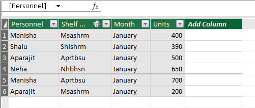
- We have a list of products, and we have a shelving code for each product. We need a table where we have the shelving description along with the shelving codes. So how do we incorporate the shelving descriptions against each shelving code? Perhaps many of us would resort to using VLOOKUP here, but we shall altogether remove the need to use VLOOKUP here using Excel Data Model.
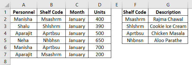
- The table on the left is the data table, and the table on the right is the lookup table. As we can see from the data, it is possible to create a relationship based on common columns.
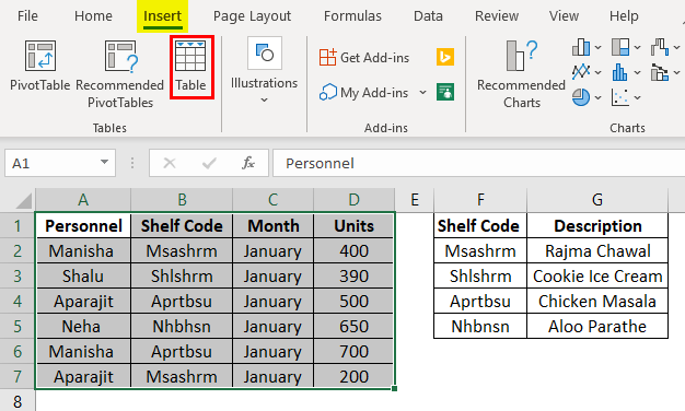
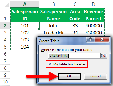
- Now, the Data Model is only compatible with table objects. So, it might be necessary sometimes to convert data sets to table objects. To do that, follow the below steps.
- Left-click anywhere in the data set.
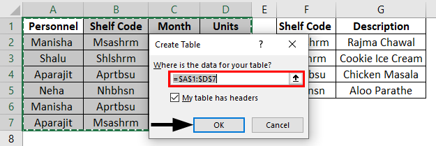
- Click the Insert tab and navigate to Table in the Tables group or simply press Ctrl+T.
- Uncheck or check the My Table has the Header option. In our example, it does indeed have a header. Click OK.
- While still focused on the new table, we need to provide a name that is meaningful in the Name box (towards the left of the formula bar).
In our example, we have named the table Personnel.
- Now we need to do the same process for the lookup table as well and name it Shelf Code.
Creating a Relationship
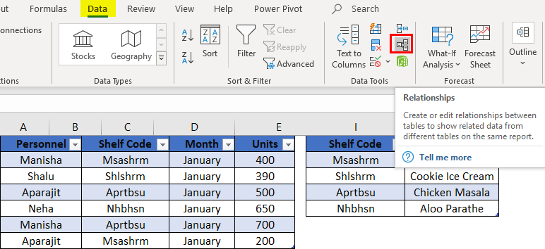
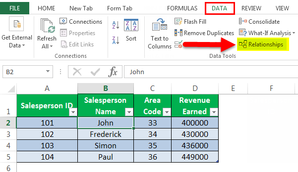
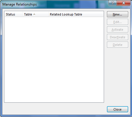
So firstly, we shall go to the Data tab and then select Relationships in the Data Tools subgroup. After we click on the Relationships option, in the beginning, since there is no relationship, hence we will have nothing.
We will first click on New to create a relationship. We will now need to provide the primary and the lookup table names from the drop-down list and then also mention the column which is common between the two tables so that we can establish the relationship between the two tables from the drop-down list of columns.
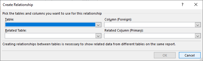
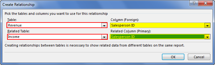
- Now, the primary table is the table that has the data. It is the primary data table – Table5. On the other hand, the Related table is the table that has the lookup data – it is our lookup table ShelfCodesTable. The primary table is the one that is analyzed based on the lookup table, which contains lookup data that will make the reported data, in the end, more meaningful.
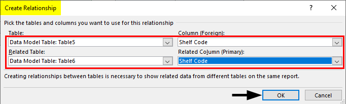
- So, the common column between the two tables is the Shelf Code column. This is what we have used to establish the relationship between the two tables. Coming to the columns, the Column (foreign) is the one that refers to the data table where there can be duplicate values. On the other hand, the Related Column (primary) refers to the column in the lookup table where we have unique values. We are simply setting up the field to lookup values from the lookup table in the data table.
- Once we set this up, Excel would create a relationship between the two behind the scene. It integrates the data and creates a data model based on the common column. This is light on the memory requirements and much faster than using VLOOKUP in large workbooks. After defining the Data model, Excel would be treating these objects as Data Model tables instead of a worksheet table.
- Now to see what Excel has been up to, we can click on Manage Data Models in Data -> Data Tools.
- We can also get the diagrammatic representation of the data model by changing the view. We will click on the View option. This will open up the view options. We will then select the Diagram View. Then we will see the diagrammatic representation, showing the two tables and the relationship between them, i.e. the common column – Shelf Code.
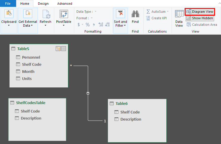
- The diagram above shows a one-to-many relationship between the unique lookup table values and the data table with duplicated values.
- Now we will have to create a pivot table. To do that, we will go to the Insert tab and then click on the Pivot Table option.
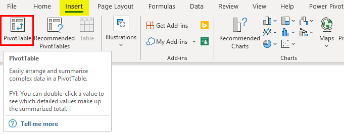
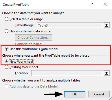
In the Pivot table’s Create Pivot Table dialogue box, we will select the source as “Use this workbook’s Data Model”.
- This will create the Pivot table, and we can see that both the source tables are available in the source section.
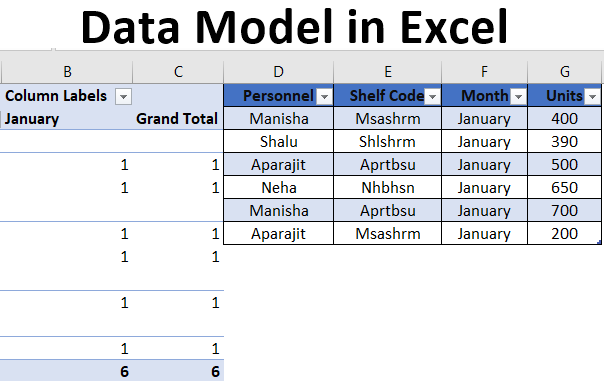
- Now we shall create a pivot table showing the count of each person who has shelved items.
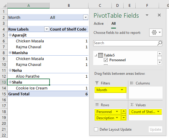
- We will select Personnel in the Rows section from Table 5 (data table), followed by Description (lookup table).
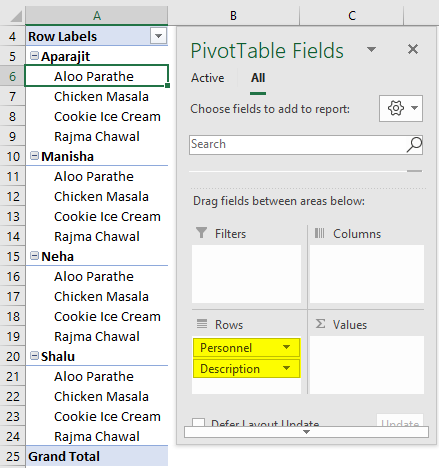
- Now we shall drag the Shelf Code from Table 5 into the Values section.
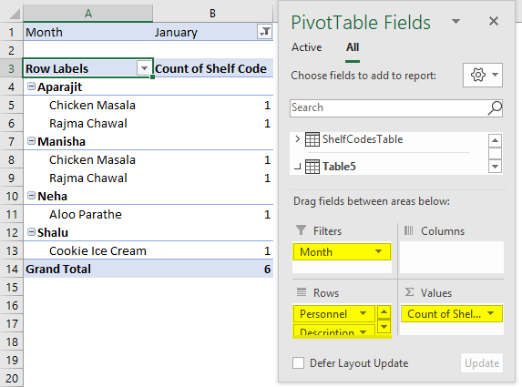
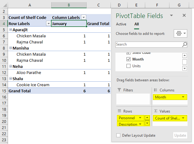
- Now we shall add Months from Table 5 to the Rows section.
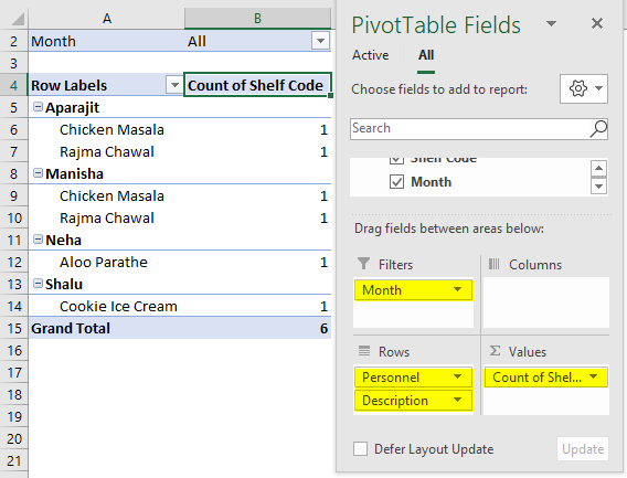
- Or we could add the months as a filter and add it to the Filters section.
Example #2
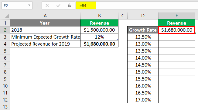
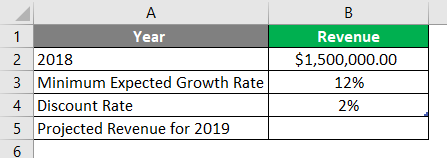
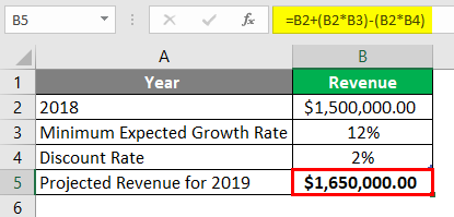
- We now have Mr Basu running a factory called Basu Corporation. Mr Basu is trying to estimate the revenue for 2019 based on the data from 2018.
- We have a table where we have the revenue for 2018 and the subsequent revenue at different incremental levels.
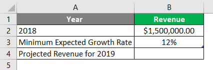
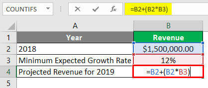
- So, we have the revenue for 2018 – $1.5 M, and the minimum growth expected the following year is 12%. Mr Basu wants a table that will show the revenue at different incremental levels.
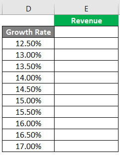
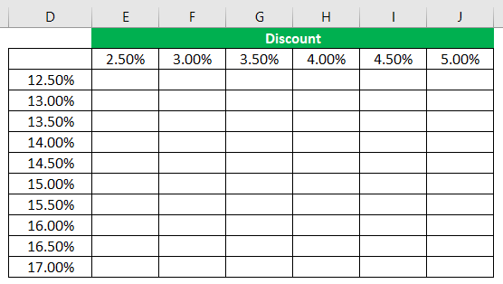
- We will create the following table for the projections at different incremental levels for 2019.
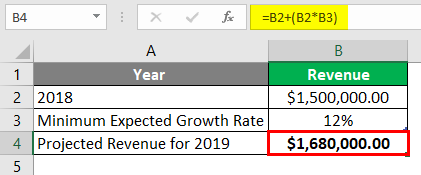
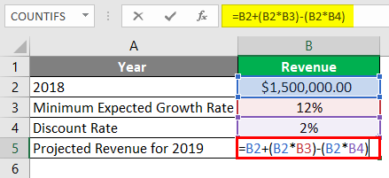
- Now we shall give the first Revenue row a reference to the estimated minimum revenue for 2019, i.e. $1.68 M.
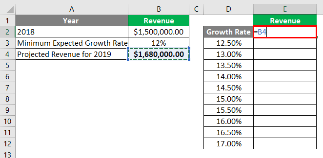
- After using the formula, the answer is shown below.
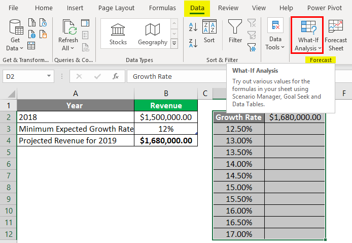
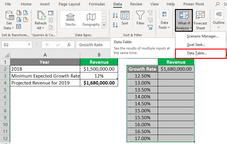
- Now we shall select the entire table, i.e. D2:E12 and then go to Data ->Forecast ->What-If Analysis ->Data Table.
- This will open up the Data Table dialog box. Here we shall enter the minimum increment percent from cell B4 in the Column Input cell. The reason for that is that our projected estimated Growth percentages in the table are arranged in a columnar fashion.
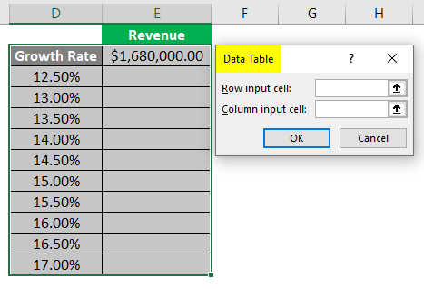
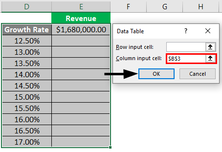
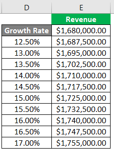
- Once we click OK, the What-If Analysis will automatically populate the table with projected revenue at the different incremental percentages.
Example #3
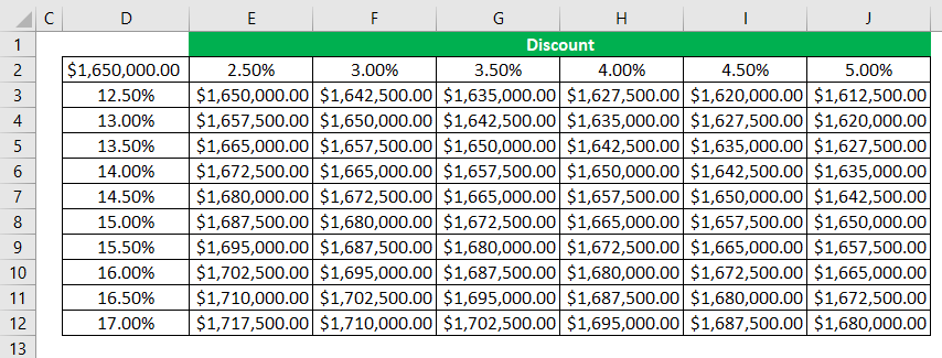
- Now suppose we have the same scenario as above, except that now we also have another axis to consider. Suppose, in addition to showing the projected revenue in 2019 based on the data of 2018 and the minimum expected growth rate, we now also have the estimated discount rate.
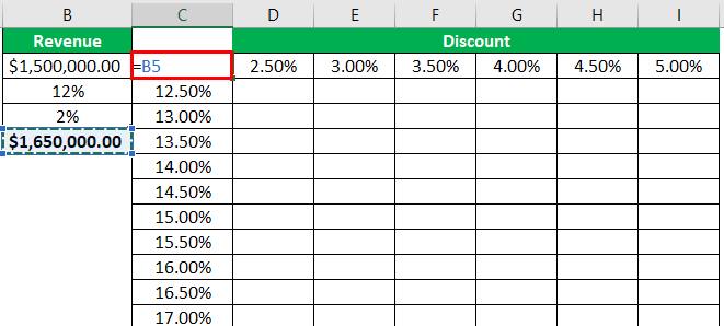
- First, we shall have a table shown below.
- Now we shall give reference to the minimum projected revenue for 2019, i.e. cell B5 to cell D8.
- Now we shall select the entire table, i.e. D8:J18 and then go to Data ->Forecast ->What-If Analysis ->Data Table.
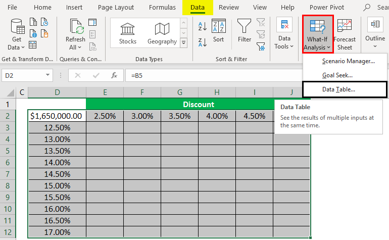
- This will open up the Data Table dialog box. Here we shall enter the minimum increment percent from cell B3 in the Column Input cell. The reason for that is that our projected estimated Growth percentages in the table are arranged in a columnar fashion. We shall now also additionally enter the minimum discount percent from cell B4 in the Row Input cell. The reason for that is that our projected discount percentages in the table are arranged in a row-wise fashion.
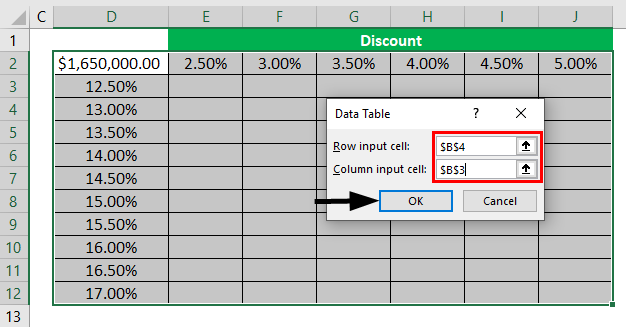
- Click OK. This will make the What-If Analysis automatically populate the table with projected revenue at the different incremental percentages as per the discount percentages.
Things to Remember About Data Model in Excel
- Upon successfully calculating the values from the data table, a simple Undo, i.e. Ctrl+Z, will not work. It is, however, possible to manually delete the values from the table.
- It is not possible to delete a single cell from the table. It is described as an array internally in Excel; hence we will have to delete all the values.
- We need to properly select the Row Input Cell and the Column Input Cell.
- The data table, unlike the Pivot Table, doesn’t need to be refreshed every time.
- Using the Data Model in Excel, we can improve performance and go easy on memory requirements in large worksheets.
- Data Models also makes our analysis much simpler as compared to using a number of complicated formulae all across the workbook.
Recommended Articles
This is a guide to Data Model in Excel. Here we discuss how to create Data Model in Excel along with practical examples and a downloadable excel template. You can also go through our other suggested articles –
- Pivot Table Slicer
- PowerPivot in Excel
- Pivot Table Formula in Excel
- Excel Pivot Table
What is the Data Model in Excel?
The data model in Excel is a type of data table where two or more two tables are in a relationship with each other through a common or more data series. In the data model, tables and data from various other sheets or sources come together to form a unique table that can access the data from all the tables.
For example, a data table containing tables of customers, product items, and product sellers. We can use the Excel data model to connect this dataset and create a relationship between them.
Table of contents
- What is the Data Model in Excel?
- Explanation
- Examples
- Example #1
- Example #2
- Things to Remember
- Recommended Articles
Explanation
- It allows integrating data from multiple tables by creating relationships based on a common column.
- Data models are used transparently, providing tabular data that can be used in a Pivot Table in ExcelA Pivot Table is an Excel tool that allows you to extract data in a preferred format (dashboard/reports) from large data sets contained within a worksheet. It can summarize, sort, group, and reorganize data, as well as execute other complex calculations on it.read more and Pivot Charts in excelIn Excel, a pivot chart is a built-in feature that allows you to summarize selected rows and columns of data in a spreadsheet. It is a visual representation of a pivot table that helps in the summarization and analysis of datasets, patterns, and trends.read more. In addition, it integrates the tables, enabling extensive analysis using pivot tables, power pivot, and Power View in ExcelExcel Power View is a data visualization technology that helps you create interactive visuals like graphs, charts. It allows you to analyze data by looking at the visuals you created. As a result, it makes your excel data more meaningful and insightful for better decision making.read more.
- The data model allows loading data into Excel’s memory.
- It is saved in memory, where we cannot directly see it. Then We can instruct Excel to relate data to each other using a common column. The ‘Model’ part of the data model refers to how all tables relate.
- The data model can access all the information it needs, even in multiple tables. After the data model is created, Excel has the data available in its memory. With the data in its memory, we can access the data in many ways.
Examples
You can download this Data Model Excel Template here – Data Model Excel Template
Example #1
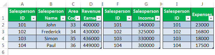
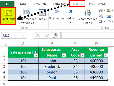
We have three datasets related to the salesperson: the first contains revenue information, the second includes the salesperson’s income and the third consists of the expenses of the salesperson.

To connect these three datasets and make a relationship with them, we make a data model with the following steps:
- Convert the datasets to table objects:
We cannot create a relationship with ordinary datasets. The data model works with only Excel TablesIn excel, tables are a range with data in rows and columns, and they expand when new data is inserted in the range in any new row or column in the table. To use a table, click on the table and select the data range.read more objects. To do this:
- Step 1 – We must first click anywhere inside the dataset, click on the “Insert” tab, and click on “Table” in the “Tables” group.
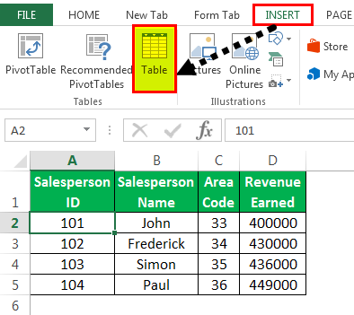
- Step 2 – Check or uncheck the ‘My table has headers’ option and click “OK.”
- Step 3 – We must enter the table’s name in the “Table Name” in the “Tools” group with the new table selected.
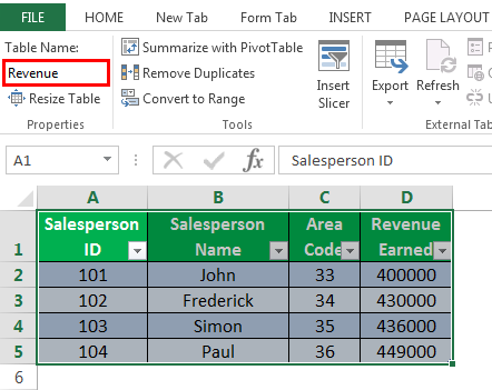
- Step 4 – Now, we can see that the first dataset is converted to a “Table” object. On repeating these steps for the other two datasets, we know that they also get converted to “Table” objects as below:
Adding the “Table” objects to the Data Model: Via Connections or Relationships.
Via Connections
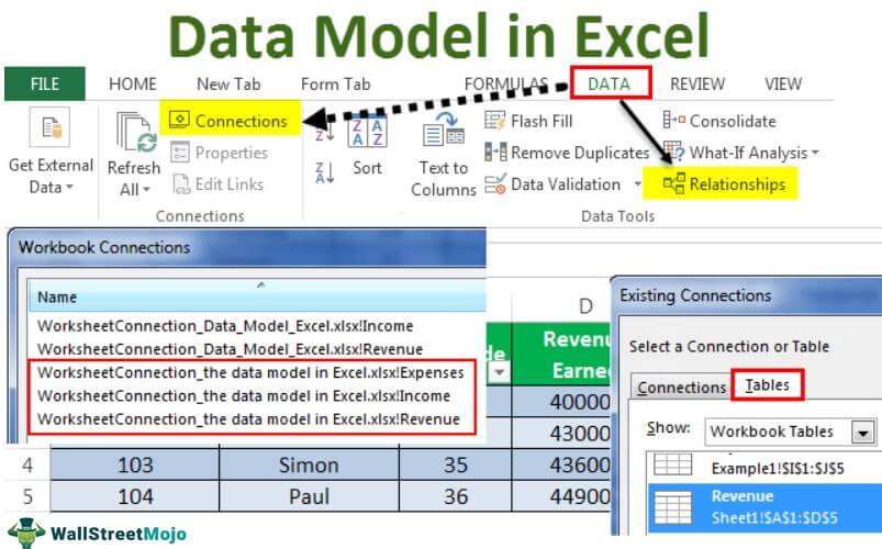
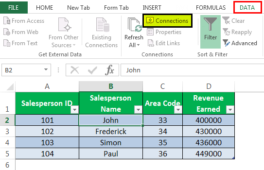
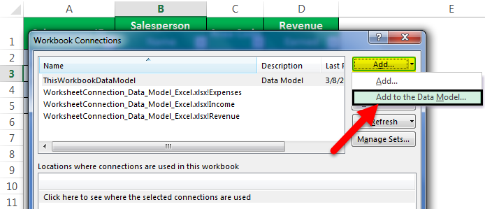
- We must select one table, click on the “Data” tab, and click on “Connections.”
- There is an icon for “Add.” Expand the dropdown of “Add” and click on “Add to the Data Model” in the resulting dialog box.
- Click on “Tables” in the resulting dialog box, select one of the tables, and click “Open.”
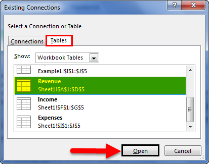
In doing this, it would create a workbook data model with one table, and a dialog box would appear as follows:
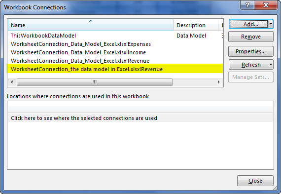
So if we repeat these steps for the other two tables, the data model will contain all three tables.
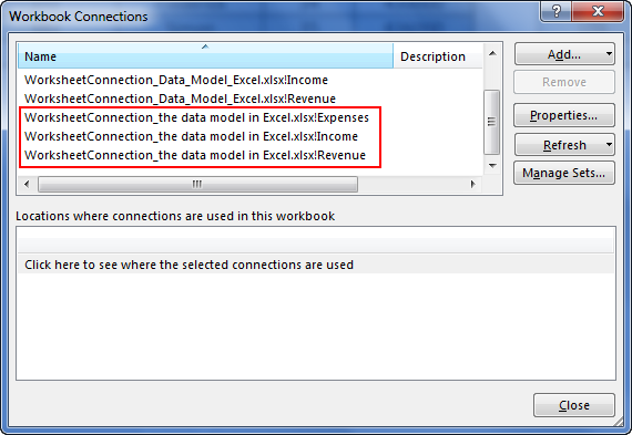
We can now see that all three tables appear in the “Workbook Connections.”
Via Relationships
Create the relationship: Once both the datasets are table objects, we can create a relationship between them. To do this:
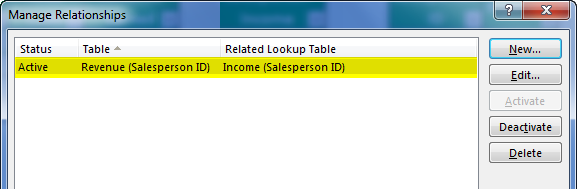
- First, we should click on the “Data” tab and “Relationships.”
- As a result, we can see an empty dialog box with no current connections.
- Then, click on “New,” and another dialog box appears.
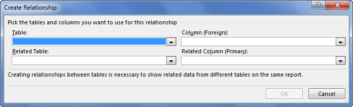
- Expand the “Table” and “Related Table” dropdowns: the “Create Relationship” dialog box appears to pick the tables and columns to use for a relationship. In the expansion of “Tables,” we must select the dataset we wish to analyze somehow, and in “Related Table,” we must choose the dataset with LOOKUP values.
- The lookup table in excelLookup tables are simply named tables that are used in combination with the VLOOKUP function to find any data in a large data set. We can select the table and name it, and then type the table’s name instead of the reference to look up the value.read more is the smaller table in the case of one to many relationships. It contains no repeated values in the common column. In expanding “Column (Foreign),” we must select the common column in the main table. In “Related Column (Primary),” we must choose the common column in the related table.
- With all these four settings selected, click on “OK.” A dialog box appears as follows on clicking on “OK.”
If we repeat these steps to relate the other two tables: the “Revenue” Table with “Expenses” table, then they also get connected in the data model as follows:
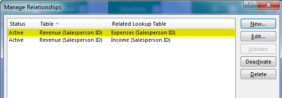
Excel now creates the relationship behind the scenes by combining data in the data model based on a common column: Salesperson ID (in this case).
Example #2
Now, in the above example, we wish to create a PivotTable that evaluates or analyzes the table objects:
- We must first click on “Insert” -> “PivotTable.”

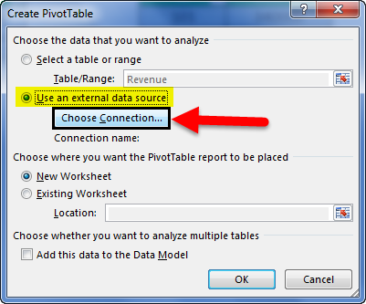
- We need to click on the “Use an external data source” option in the resulting dialog box and click on “Choose Connection.”

- Then, we must click on “Tables” in the resulting dialog box, select the “Workbook Data Model” containing three tables, and click “Open.”

- Select the “New Worksheet” option in the location and click on “OK.”
- Consequently, the “PivotTable Fields” pane will display table objects.

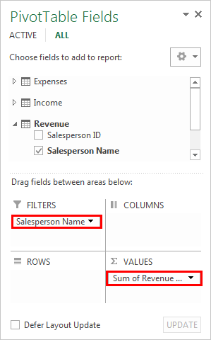
Now we can make changes in the PivotTable accordingly to analyze the table objects as required. - For instance, in this case, if we wish to find the total revenue or revenue for a particular salesperson, then a PivotTable is created as follows:


It is an immense help in the case of a model/table containing a large number of observations.


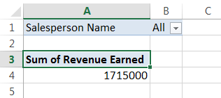
So, we can see that the pivot table instantly uses the data model (picking it by choosing connection) in Excel memory to show relationships between tables.
Things to Remember
- We can analyze data from several tables at once using the data model.
- By creating relationships with the data model, we surpass the need for using VLOOKUPThe VLOOKUP excel function searches for a particular value and returns a corresponding match based on a unique identifier. A unique identifier is uniquely associated with all the records of the database. For instance, employee ID, student roll number, customer contact number, seller email address, etc., are unique identifiers.
read more, SUMIF, INDEX functionThe INDEX function in Excel helps extract the value of a cell, which is within a specified array (range) and, at the intersection of the stated row and column numbers.read more, and MATCH formulas as we do not need to get all columns within a single table. - Models are implicitly created when datasets are imported in Excel from outside sources.
- We can create table relationships automatically if we import related tables with primary and foreign key relationships.
- While creating relationships, the columns that we are connecting in tables should have the same data type.
- With the pivot tables created with the data model, we can add slicers and slice them on any field at pivot tables we want.
- The advantage of the Data Model over LOOKUP() functionsThe LOOKUP excel function searches a value in a range (single row or single column) and returns a corresponding match from the same position of another range (single row or single column). The corresponding match is a piece of information associated with the value being searched.
read more is that it requires substantially less memory. - Excel 2013 supports only one-to-one or one to many relationships, i.e., one of the tables must have no duplicate values on the column we are linking to.
Recommended Articles
This article is a guide to Data Model in Excel. We discuss creating a data model from Excel tables using connections and relationships, practical examples, and a downloadable Excel template. You may learn more about Excel from the following articles: –
- Excel Value Formula
- Excel MATCH Formula
- Share an Excel Workbook
- Consolidate Data in Excel
The following post is the third in a series of posts about Excel Model Building. To review the previous posts on this topic, please click through the links below:
Click here for Part 1 of this post, How to Build an Excel Model: Key Principles
Click here for Part 2 of this post, How to Build an Excel Model: Tab Structure
Now that we’ve learned the key principles of model building, as well as a general tab structure, this final part of the Excel model building tutorial will review a step by step example of building a model from the ground up. The direction is still somewhat high level, but I’ve included a sample model that follows the prescribed guidelines. The model has already been built to completion, but it can be used to help you follow along and provide context for the high level steps referenced.
Click below to download the sample model:
MBA Excel Sample Model v1.0
Click here to view the supporting documentation for MBA Excel Sample Model
Step 1: Build Output Tabs Shell – Understand Your Requirements
Most people who’ve implemented software will tell you that the majority of errors occur during the requirements gathering phase of the project. (For those of you who haven’t done an implementation, this is the phase of the project where you figure out what your software actually needs to do) Excel model building faces the exact same issue. Before you start building, you should figure out what outputs your model needs to generate. These requirements will greatly influence every subsequent step you take. For example, if you need to build multiple scenarios, you may need to leave space to input different scenario assumptions. If you need to conduct sensitivity analysis, then you may need to use Excel Data Table or build a sensitivity tornado chart.
Understanding your exact requirements first is not always possible, but you should always try to be as definitive as you can. The worst case scenario is investing several hours into building a model that can’t generate the type of outputs you actually need.
In this adjusted snapshot of the sample model, you can see here that the requirements are to build a five your P&L forecast. In the model download, you’ll note that I’ve also included a “Sales Revenue by City” report as an additional requirement.

Step 2: Build Calculations on Paper – Determine Inputs Required
It’s always tempting to jump right into Excel to start building your model immediately. But whenever you’re dealing with a really complex model, it’s always useful to step back with just a pen and paper to sketch out your intended plan. While not everyone uses this step, it can definitely help you gain perspective on your work and prevent you from missing critical ideas.
Step 3: Build Input Tabs and Gather the Required Values
Once you’ve sketched out your calculations, you should have a pretty good idea of what inputs you need to build your model. As mentioned in the tab structure post, you can have three kinds of inputs: drivers, static inputs, and data tables. As a best practice, you should try to ensure that all of your inputs are in as few tabs as possible, with the minor exception of breaking them up into different tabs between these three categories. This is critical because one of the biggest transparency complaints people have when dealing with second hand models is that they can’t find out where they’re supposed to input values.
On many occasions, you won’t have the actual input value you need when you begin building your model. In this situation, it’s best to input a dummy figure, or some rough historical average, so you can continue the model building process. Just make sure to add a notation so you remember to come back and update it.
The example below shows the Drivers tab within the sample model.

Step 4: Load Data Tables
Data tables represent a slightly more complex input than drivers or static inputs. As a general rule, any table that has more rows and / or columns that you can fit and view on your laptop screen deserves its own tab. Make sure that you use proper database formatting for these tables, as it is very possible that someone will take the table and load it into another file in the future.
In the sample model, we have a data table representing Total Product Sales by Territory in 2013.

Step 5: Build Calculations off of Inputs, Drivers, and Data Tables
At this point we’ve finished most of the setup tasks for model building and are ready to get into the heart of the exercise. Your knowledge of database theory and Excel formulas will definitely come in handy here. The calculation tabs are probably the least uniform aspect of Excel models. This is because, for any given goal, there are several ways to get to your solution. While it would be ideal to build your model in the most efficient way possible during your first try, this is rarely possible. The fact is good model building requires trial and error. Only by going through different iterations of your model can you create the best possible outcome.
One best practice to keep in mind is that you should try to do most of your calculations in your calculation tabs and not in your output tabs. While it can definitely be faster to do calculations in the output tabs, it may make it harder for someone to audit your file in the future. By keeping all calculations in a defined area, you’ll significantly increase both the consistency and the transparency of your file. The major exception to this rule is if you’re just doing a sum, count, or lookup. Since these formulas summarize your data, they are appropriate for the output section.
Step 6: Link Calculated values to Output Tabs and Finalize Formatting of Output Tabs
By now the data you’ve run your calculations and should be very close to the exact values you need in your output tabs. You may still need to use some summary formulas to arrange your data based on your initial requirements. Since the output tabs are primarily for display, take time to format these for printing and apply Visual Design techniques. Additionally, make them as transparent as possibly by including sources, unit values, and any other beneficial documentation.
Step 7: Build Your Index Tab
At this point, you should have the majority of your tabs in place for your model. Building your Index Tab will significantly help summarize the scope and functionality of your model. Make sure that every tab you’ve created is documented and described. If you realize that any tabs are unnecessary, remove them. You will probably need to update this tab periodically if any aspect of your model changes.
I always find it useful to hyperlink the tab descriptions to the actual tabs they are describing to enhance the navigation within the model. You can see an example below of the Index Tab for the sample model.

Step 8: Link Key Output Values to Drivers Tab to Perform Scenario and Sensitivity Analysis
As you get towards the end of the model building process, it’s very likely that you’ll want to conduct some form of scenario or sensitivity analysis. To prepare for this step, you should determine what output values are the most important to your analysis and link them back to your drivers tab. The process for doing so is relatively simple and shouldn’t take much more than using the equals sign to write a simple linking formula.
Additionally, you’ll obviously need to understand which of your drivers are most likely to change and have a reasonable range of possible values for these variables. These factors will be completely dependent on the specific type of model you are building.
Another potential option for sensitivity analysis is to use Excel’s Watch Window feature. While this is a great tool for sensitivity specifically, linking your output values to the drivers tab is the best way to create defined scenarios.

Step 9: Create Documentation and Finish Index Tab
As I’ve mentioned before, few Excel models ever have adequate documentation. This additional step adds to your workload and no one really enjoys doing it. However, having documentation can make a huge difference to whomever you might hand your off work to. I like to think of documentation as an insurance policy; put in a little work now, and you’ll significantly reduce the need to answer questions in the future. You’ll also be much less likely to forget your own methodology if you ever need to come back to your file.
Documentation doesn’t have to be a long winded user guide that takes several hours to write. It can take the form of comment boxes in cells, notes in formulas, or just a separate tab in the Excel document explaining your assumptions. All of these things further the transparency of your model and should be included if possible.
For the sample model, I’ve included the documentation as a linked web page, in case it needs to be updated in the future.
Step 10: Add Cell & Workbook Protection Where Appropriate
This last step is important if you plan to either widely distribute your file or solicit inputs from your colleagues. This is especially important in the latter scenario because before you save a new version of your file, you want cell protection in areas that should not be adjusted as well as a clear understanding of what sections your colleagues had the ability to change. The process of protecting your file is fairly simple: you just need to choose which cells will be editable by other users and then assign a password to your workbook.
You’ll notice in the sample model, I’ve protected the Index Tab where the link to the documentation exists. That way, it reduces the likelihood that this sample model will be sent out without the accompanying documentation.
Click here for Part 1 of this post, How to Build an Excel Model: Key Principles
Click here for Part 2 of this post, How to Build an Excel Model: Tab Structure