How to merge data in excel

If you receive information in multiple sheets or workbooks that you want to summarize, the Consolidate command can help you pull data together onto one sheet. For example, if you have a sheet of expense figures from each of your regional offices, you might use a consolidation to roll up these figures into a corporate expense sheet. That sheet might contain sales totals and averages, current inventory levels, and highest selling products for the whole enterprise.

To decide which type of consolidation to use, look at the sheets you are combining. If the sheets have data in inconsistent positions, even if their row and column labels are not identical, consolidate by position. If the sheets use the same row and column labels for their categories, even if the data is not in consistent positions, consolidate by category.

Combine by position

For consolidation by position to work, the range of data on each source sheet must be in list format, without blank rows or blank columns in the list.

1. Open each source sheet and make sure that your data is in the same position on each sheet.

2. In your destination sheet, click the upper-left cell of the area where you want the consolidated data to appear.

   Note: Make sure that you leave enough cells to the right and underneath for your consolidated data.

3. On the Data tab, in the Data Tools group, click Consolidate.

   

4. In the Function box, click the function that you want Excel to use to consolidate the data.

5. In each source sheet, select your data.

   The file path is entered in All references.

6. When you have added the data from each source sheet and workbook, click OK.

Combine by category

For consolidation by category to work, the range of data on each source sheet must be in list format, without blank rows or blank columns in the list. Also the categories must be consistently labeled. For example, if one column is labeled Avg. and another is labeled Average, the Consolidate command will not sum the two columns together.

1. Open each source sheet.

2. In your destination sheet, click the upper-left cell of the area where you want the consolidated data to appear.

   Note: Make sure that you leave enough cells to the right and underneath for your consolidated data.

3. On the Data tab, in the Data Tools group, click Consolidate.

   

4. In the Function box, click the function that you want Excel to use to consolidate the data.

5. To indicate where the labels are located in the source ranges, select the check boxes under Use labels in: either the Top row, the Left column, or both.

6. In each source sheet, select your data. Make sure to include either the top row or left column information that you previously selected.

   The file path is entered in All references.

7. When you have added the data from each source sheet and workbook, click OK.

   Note: Any labels that don’t match labels in the other source areas cause separate rows or columns in the consolidation.

Combine by position

For consolidation by position to work, the range of data on each source sheet must be in list format, without blank rows or blank columns in the list.

1. Open each source sheet and make sure that your data is in the same position on each sheet.

2. In your destination sheet, click the upper-left cell of the area where you want the consolidated data to appear.

   Note: Make sure that you leave enough cells to the right and underneath for your consolidated data.

3. On the Data tab, under Tools, click Consolidate.

   

4. In the Function box, click the function that you want Excel to use to consolidate the data.

5. In each source sheet, select your data, and then click Add.

   The file path is entered in All references.

6. When you have added the data from each source sheet and workbook, click OK.

Combine by category

For consolidation by category to work, the range of data on each source sheet must be in list format, without blank rows or blank columns in the list. Also the categories must be consistently labeled. For example, if one column is labeled Avg. and another is labeled Average, the Consolidate command will not sum the two columns together.

1. Open each source sheet.

2. In your destination sheet, click the upper-left cell of the area where you want the consolidated data to appear.

   Note: Make sure that you leave enough cells to the right and underneath for your consolidated data.

3. On the Data tab, under Tools, click Consolidate.

   

4. In the Function box, click the function that you want Excel to use to consolidate the data.

5. To indicate where the labels are located in the source ranges, select the check boxes under Use labels in: either the Top row, the Left column, or both.

6. In each source sheet, select your data. Make sure to include either the top row or left column information that you previously selected, and then click Add.

   The file path is entered in All references.

7. When you have added the data from each source sheet and workbook, click OK.

   Note: Any labels that don’t match labels in the other source areas cause separate rows or columns in the consolidation.

Every day, most analysts merge data in Excel and other spreadsheet programs to get better insights. Consolidating data in Excel is part of a bigger process called data preparation, but as the number of new data sources increases, if you want to merge data in excel spreadsheets, it is getting harder to do.

At Trifacta we are passionate about creating radical productivity for business analysts, so we became experts in data preparation. Even though we make software that replaces Excel in some cases, inside our company we still merge data in Excel just like you do, because sometimes it’s still the right tool for the right job. So, we know from firsthand experience when consolidating data in excel with a spreadsheet is a good idea, and how to do it well.

As it turns out,  the terms “Merge” and “Consolidate” in Excel, refer to two separate functions. Because of that, we created a short guide to understanding them both, as well as what to do when consolidating data in Excel is no longer an option.

How to Consolidate Data in Excel

For this example, let’s say you are given two sets of data about the amount of loans a group of members have borrowed per year, each in an independent Excel workbook. You want to understand the total amount of loans borrowed by each member, so you may naturally wonder how to combine data in Excel.

If both sets of numeric data are already formatted in a similar way, such as prices always formatted as $1.00, you can use the Excel consolidate feature (under the ‘Data’ dropdown menu).

Open each sheet you plan to use and confirm that the data types you want to consolidate in Excel match.

1. In a new empty worksheet, select ‘Consolidate.’
2. In the ‘Function’ box, select the function you want to use. In this example, we’re using “Sum” to add together the total loans borrowed per member. 
3. Under ‘Reference,’ select ‘Browse’ to identify the Excel workbooks you want to consolidate the data from. Add the source(s).
4. Important: Make sure the labels match. Then hit ‘OK,’ watch the data propagate, and begin reviewing or analyzing the new sheet.

How to Merge Data from Two Excel Worksheets

Traditionally, VLookup has been one of the most important tools for merging data in Excel, but the process requires multiple steps and can easily tire analysts who must merge multiple columns across many datasets. Instead, let’s take a look at how we can do this same process all within the Excel Power Query editor. 

In this example, we’re using two individual datasets, the first containing basic member information, such as income, education, phone number, etc., and the second containing member loan information, such as the loan amount, interest rate, loan status, etc. Each dataset also contains a member ID, which will allow us to join the data on that common field in order to compare all of this data side by side. Here’s how to proceed:

1. First, we’ll take a look at each dataset to roughly analyze their contents, and then open up a new worksheet for our merged dataset. 
2. Next, we’ll click on the “Data” tab of our new worksheet and select “From Text/CSV” because the files that we’re working with are csv files. You can also import Excel files by selecting “Get Data.” 
3. We’ll start by importing our file on basic member info, which will bring us into the Power Query editor. 
4. Next, we’ll bring in our other dataset by selecting “New Source” and “Text/CSV” and we’ll see the dataset on loan information added to the left-hand side. 
5. To merge these two datasets, we’re going to select “Merge Queries” and “Merge as New” so that we can have a separate space for our new dataset. 
6. We know that the common data field is “member ID” so we’re going to select that column for both datasets. 
7. Now, we’re going to delete some of the columns that we don’t need from our member information dataset. When we’re finished, we’re going to click on the icon next to “member_loans” to expand the dataset we just brought in. 
8. Here, we’re going to select the columns that we want from our member loans dataset. We don’t need to bring in member ID, as it’s already a column in our member info dataset. 
9. Once we’re finished selecting, we can rearrange these columns as it makes sense for our analysis. 
10. And finally, we’ll hit “Close and Load” to see the finished, merged dataset in our blank worksheet.

Merge Data In Excel with Designer Cloud

As the scale and complexity of your data sources grow, you might find merging data with Excel is harder to do. For large and varied data sets, Excel becomes too complicated, cumbersome and slow to use when you are trying to merge data in Excel. That’s where Designer Cloud comes in. Designer Cloud is specifically designed to make this preparation process easier and more intuitive.

For example, imagine being able to save the specific merge functions you use to merge data in Excel, customized to each unique data source,  and then reuse and share them with your colleagues effortlessly.

With Designer Cloud, data preparation is accessible, intuitive, and scalable across the organization. By providing a connected application for users to explore, structure, and produce dashboard-ready datasets, Designer Cloud helps users deliver faster, more accurate analysis.

Designer Cloud was designed from the ground up to help reduce data cleansing and data preparation time. At Alteryx, we live and breathe data in order to provide easy-to-use, intelligent, visual data analysis that improves data understanding for any project or organization. Sign up for Free Designer Cloud today.

A good database is always structured. It means different entities have different tables. Although, Excel is not a database tool but is often used to maintain small chunks of data.

Many times we get the need of merging tables in order too see a relationship and churn out some useful information.

In databases like SQL, Oracle, Microsoft Access, etc, it is easy to join tables using simple queries. But in excel we don’t have JOINs but we can still join tables in excel. We use Excel Functions to merge and join data tables. Perhaps it is a more customizable merge than SQL. Let’s see the techniques of merging excel tables.

Merge Data in Excel Using VLOOKUP Function

To merge data in excel, we should have at least one common factor/id in both tables, so that we can use it as a relation and merge those tables.
Consider these two tables below. How can we combine these data tables in Excel?

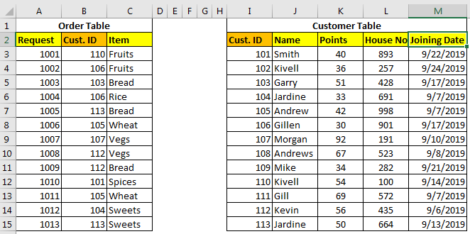
The Order Table has order details and the Customer table contains customer details. We need to prepare a table that tells which order belongs to which customer name, customer’s points, house number, and his joining date.

The common id in both tables is Cust.ID which can be used for merging tables in excel.

There are three methods of merging tables using VLOOKUP Function.

Retrieve Each Column With Column Index

In this method, we will use simple VLOOKUP to add these tables in one table. So to retrieve name write this formula.

[Customers is Sheet1!$I$3:$M$15.]

=VLOOKUP(B3,Customers,2,0)

To merge points in table, write this formula.

=VLOOKUP(B3,Customers,3,0)

To merge house no in table, write this formula.

=VLOOKUP(B3,Customers,4,0)

Here we merged two tables in excel, each column one by one in the table. This is useful when you have only few columns to merge. But when you have multiple columns to merge, this is can be a hectic task. So to merge multiple tables we have different approaches.

Merge Tables Using VLOOKUP and COLUMN Function.

When you want to retrieve multiple adjacent columns, use this formula.

=VLOOKUP(lookup_value,table_array,COLUMN()-n,0)

Here the COLUMN function just returns the column numbers in which the formula is being written.

n is any number which adjusts the column number in table array,

In our example, the formula for table merging will be:

=VLOOKUP($B3,Customers,COLUMN()-2,0)

Once you write this formula, you will not have to write the formula again for other columns. Just copy it in all other cells and columns.

How It Works

Ok! In the first column, we need a name, which is the second column in customer table.

Here the main factor is COLUMN()-2. The COLUMN function returns the column number of current cell. We are writing the formula in D3, hence we will get 4 from COLUMN(). Then we are subtracting 2 which makes 2. Hence finally our formula simplifies to =VLOOKUP($B3,Customers,2,0).

When we copy this formula in E columns we will get the formula as =VLOOKUP($B3,Customers,3,0). Which retrieves 3rd column from customer table.

Merge Tables Using VLOOKUP-MATCH Function
This one is my favorite way of merging tables in excel using the VLOOKUP function. In the above example, we retrieved column in serial. But what if we had to retrieve random columns. In that case above Techniques will be useless. The VLOOKUP-MATCH technique uses column headings to merge cells. This is also called VLOOKUP with Dynamic Col Index.

For our example here, the formula will be this.

=VLOOKUP($B3,Customers,MATCH(D$2,$J$2:$N$2,0),0)

Here, we are simply using MATCH function to get the appropriate column number. This called Dynamic VLOOKUP.

Using INDEX-MATCH to Table Merging in Excel
The INDEX-MATCH is very powerful lookup tool and many time it is referred as better VLOOKUP function. You can use this to for combining two or more tables. This will also allow you to merge columns from left of the table.

This was a quick tutorial about merging and joining tables in excel. We explored several ways of merging two or more tables in excels. Feel free to ask question about this article or any other query regarding excel 2019, 2016, 2013 or 2010 in the comments section below.

Related Articles:

IF, ISNA and VLOOKUP function in Excel

IFERROR and VLOOKUP function in Excel

How to retrieve the entire row of a matched value in Excel

Popular Articles :

50 Excel Shortcut to Increase Your Productivity : Get faster at your task. These 50 shortcuts will make you work even faster on Excel.

How to use the VLOOKUP Function in Excel : This is one of the most used and popular functions of excel that is used to lookup value from different ranges and sheets.

How to use the COUNTIF function in Excel : Count values with conditions using this amazing function. You don’t need to filter your data to count specific values. Countif function is essential to prepare your dashboard.

How to use the SUMIF Function in Excel : This is another dashboard essential function. This helps you sum up values on specific conditions.

Summary:

Does merging rows and columns in Excel seems a tough task for you to perform? Read this tutorial to learn different ways to merge rows and columns in Excel.

Microsoft Excel is a very useful application and can be used for performing various tasks. This is the reason Excel provides various useful functions to make the task easy for the users.

One of the most common tasks that everyone needs performing now and then is merging rows and columns.

But the problem is that performing this is not an easy task and Excel does not provide any tool to do this.

This is quite complicated as merging rows and columns in some cases causes data loss.

As while trying to combine two or more rows in the worksheet by making use of the Merge & Center button (Home tab > Alignment group), you will start getting the error message:

“The selection contains multiple data values. Merging into one cell will keep the upper-left most data only.”

And if you click OK, merged cells would contain just the value of the top-left cell and as a result, entire other data will be removed.

So this is what leads you to Panic situation!!!

To get rid of this, today in this article I am sharing different ways to easily merge rows and columns in excel without losing any data.

Below check out the fixes on how to merge rows in Excel or how to merge columns in Excel.

There are different methods for combining row and columns text in Excel. Here check the ways one by one to merge data without losing it. First, check how to merge rows in Excel.

Part 1# How To Merge Rows in Excel

When it comes to merging the Excel rows there are two ways that allow you to merge rows data easily.

1. Merge Excel rows using a formula
2. Combine multiple rows using the Merge Cells add-in

1. How to Merge Multiple Rows using Excel Formulas

Excel provides various formulas that help you combine data from different rows. Possibly the easiest one is the CONCATENATE function. So here checks out some examples for concatenating numerous rows into one:

• Merge rows with spaces between data: For example =CONCATENATE(B1,” “,B2,” “,B3)
• Combine rows without any space between the values: For example =CONCATENATE(A1,A2,A3)
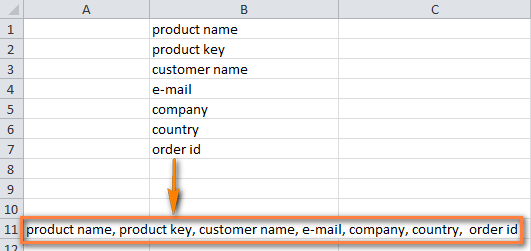
• Merge rows > separate the values with comma: For Example =CONCATENATE(A1,”, “,A2,”, “,A3)

Now check how the CONCATENATE formula works on the real data.

• On the sheet choose an empty cell and type the formula into it. Type the formula as per the data rows
• And copy the formula across entire other cells in the row.

• Now, simply you are having several data rows merged into one row.

2. How to Combine Rows in Excel using the Merge Cells Add-in

The Merge Cells add-in is used for merging various types of cells in Excel. This allows you to merges the individual cells and also combines data from entire rows or columns.

Please Note: You need to download a merge cell add-ins for third-party sites available online. Search in Google for add-ins.

Follow the given steps to combine two or more rows in your table:

1. Choose rows you are looking to merge > click on the Merge Cells icon.
2. Now the merge cells dialog window opens with a table or range selected already. And in the upper part of the window, you can see the three basic things:

• • How you want to join cells – For combining rows of data > choose “column by column“.
  • How to separate merged values with – an array of standard separators is available to choose from > comma, space, semicolon, and a line break. So select the separator as per your desire.
  • Where you need to place the merged cells > either the top cell or bottom cell.

1. Now check the lower part of the Windows to check if you need any additional options:

• • Clear the content of selected cells – Choose this if need data to remain in the merged cells only.
  • Merge all areas in the selection – This option allows you to merge rows in two or more non-adjacent ranges.
  • Skip empty cells and Wrap text – Well, these are self-explanatory.
  • Lastly, Create a backup copy of the worksheet – This option is checked by default.  It is just a precaution that keeps you on the safe side and prevents the risk of data loss.

1. Click the Merge button > to check the result – possible the merged rows of data separated by line breaks.

So, these are the two ways that allow you to merge rows in Excel without any data loss. Now, check out the ways on how to combine two columns in Excel.

Part 2# How To Merge Columns In Excel 

Here check out the 3 ways to merge data from several columns into one without using VBA macro.

• Merge two columns using formulas
• Combine columns data via NotePad
• The fastest way to join multiple columns

1. Merge Two Columns using Excel Formulas

1. Into your table > insert a new column > in the column header place the mouse pointer > right-click the mouse > select Insert from the context menu. Name the newly added columns for eg. – “Full Name”

2. In the cell D2, write the formula: =CONCATENATE(B2,” “,C2). The B2 and C2 are the addresses of First Name and Last Name. And in the formula, the quotation marks “” is the separator that will be inserted between merged names any other symbol can be used as a separator e.g. a comma.

3. Just like this, join data from several cells into one by making use of any separator of your choice.

4. Simply, copy the formula to other cells of the Full Name column. If the First name or the Last name is deleted, then the corresponding data in the Full name Column will also be gone.

5. Next, try converting the formula to a value so that you can remove the unnecessary columns from the Excel worksheet. Choose entire cells with data in the merged column (choose the first cell in “Full Name” Column > press Ctrl +Shift + Arrow Down)

6. Now copy the contents of the columns to clipboard > right click on the cell in the same column (“Full Name”) > choose “Paste Special” context menu > choose “Values” radio button > click OK.

7. Now remove “First Name” & “Last Name” columns that are not required. Click the column B header > press and hold Ctrl > click column C header.

8. After that make a right-click on any selected columns > select Delete from the context menu.

9. This is it, now you have successfully merged the names from 2 columns into one.

2. Combine columns Data via Notepad

This is another way that allows you to merge several columns. Here you don’t need any formulas. This is suitable for combining adjacent columns to make use of the same delimiter for all of them.

For Example: If looking for combining 2 columns with First Names and Last Names into one:

1. Choose both columns you need to merge: Click B1 > press Shift + ArrrowRight for choosing C1 > then hit Ctrl + Shift + ArrowDown for choosing entire data cells with data in two columns.

• And copy data to clipboard > open Notepad > insert data from the clipboard to the Notepad

• Then copy tab character to clipboard > hit Tab right in Notepad > hit Ctrl + Shift + LeftArrow > press Ctrl + X.
• After that Replace Tab characters in Notepad with the separator, you require.
• Hit Ctrl + H for opening the “Replace” dialog box > paste the Tab character from the clipboard in Find what field > type the separator Space, comma etc in “Replace with” field. Hit the Replace All button > to close the dialog box press Cancel

• Now select the entire text in the Notepad and copy it to Clipboard.
• Then switch back to Excel worksheet (press Alt + Tab) > choose B1 cell and paste text from Clipboard to your table.

• And rename column B to “Full Name“ and remove the “Last name” column.

So, this is the second way that allows you to merge columns in Excel without any data loss.

3. Join Columns Using Merge Cells Add-in For Excel

This is the easiest and quickest way for combining data from numerous Excel columns into one. Just make use of the third party merge cells add-in for Excel.

And with the merge cells add-in you can merge data from many cells by using any separator you like (for example carriage return or line break). With this, you can join row by row, column by column, or merge data from the selected cell into one without any loss.

There are many third-party add-ins online sites that allow you to download the add-ins and merge the cells easily in just a few clicks.

Conclusion:

So this is all about merging rows and columns in Excel without any data loss.

Follow the given steps to combine text in rows and columns easily.

Hope the given different steps will allow you to perform the task easily in the rows and column. Here I have described different methods of merging rows and columns data in Excel without any data loss.

So make use of anyone that you find easy for you.

However if in case you come to face any issue or data loss situation in Excel then make use of the MS Excel Repair Tool. This is the best tool that allows you to repair and recover data from the corrupted, damaged Excel file.

Additionally, you can learn advanced Excel to become more productive and easily utilize Excel functions and formulas.

Related articles

Faster with Excel: the VLOOKUP function explained

It can often be incredibly time-consuming to search for a specific entry in an Excel table by hand, which is where VLOOKUP comes into play. This practical function allows you to find the exact value for a specific search criterion. The VLOOKUP function is indispensable for managing price lists, members directories, and inventory catalogues. To ensure you can benefit from this practical function,…

Faster with Excel: the VLOOKUP function explained

An overview of Excel formulas and functions

There are many Excel functions and formulas that are useful for a wide range of tasks. They can help you make your workflows easier and more efficient. We’ll introduce you to the most important ones here, and you’ll be on your way to being an Excel expert.

An overview of Excel formulas and functions