
Create and build a custom numeric format to show your numbers as percentages, currency, dates, and more. To learn more about how to change number format codes, see Review guidelines for customizing a number format.

-
Select the numeric data.
-
On the Home tab, in the Number group, select the small arrow to open the Dialog box.

-
Select Custom.
-
In the Type list, select an existing format, or type a new one in the box.
-
To add text to your number format:
-
Type what you want in quotation marks.
-
Add a space to separate the number and text.
-
-
Select OK.
Excel provides many options for displaying numbers in different formats like percentages, currency, and dates. If the built-in formats don’t work for your needs, you might want to create a custom number format.
You can’t create custom formats in Excel for the web but if you have the Excel desktop application, you can click the Open in Excel button to open the workbook and create them. For more information, see Create a custom number format.
Содержание
- Available number formats in Excel
- Number formats
- Need more help?
- Add numbers in Excel 2013
- Want more?
- Convert numbers stored as text to numbers
- 1. Select a column
- 2. Click this button
- 3. Click Apply
- 4. Set the format
- Other ways to convert:
- 1. Insert a new column
- 2. Use the VALUE function
- 3. Rest your cursor here
- 4. Click and drag down
- Custom Excel number format
- How to create a custom number format in Excel
- Understanding Excel number format
- Excel formatting rules
- Digit and text placeholders
- Excel formatting tips and guidelines
- How to control the number of decimal places
- How to show a thousands separator
- Round numbers by thousand, million, etc.
- Text and spacing in custom Excel number format
- Including currency symbols in a custom number format
- How to display leading zeros with Excel custom format
- Percentages in Excel custom number format
- Fractions in Excel number format
- Create a custom Scientific Notation format
- Show negative numbers in parentheses
- Display zeroes as dashes or blanks
- Add indents with custom Excel format
- Change font color with custom number format
- Repeat characters with custom format codes
- How to change alignment in Excel with custom number format
- Apply custom number formats based on conditions
- Dates and times formats in Excel
Available number formats in Excel
In Excel, you can format numbers in cells for things like currency, percentages, decimals, dates, phone numbers, or social security numbers.
Select a cell or a cell range.
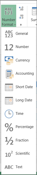
On the Home tab, select Number from the drop-down.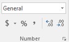
Or, you can choose one of these options:
Press CTRL + 1 and select Number.
Right-click the cell or cell range, select Format Cells… , and select Number.
Select the small arrow, dialog box launcher, and then select Number.
Select the format you want.
Number formats
To see all available number formats, click the Dialog Box Launcher next to Number on the Home tab in the Number group.

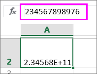
The default number format that Excel applies when you type a number. For the most part, numbers that are formatted with the General format are displayed just the way you type them. However, if the cell is not wide enough to show the entire number, the General format rounds the numbers with decimals. The General number format also uses scientific (exponential) notation for large numbers (12 or more digits).
Used for the general display of numbers. You can specify the number of decimal places that you want to use, whether you want to use a thousands separator, and how you want to display negative numbers.
Used for general monetary values and displays the default currency symbol with numbers. You can specify the number of decimal places that you want to use, whether you want to use a thousands separator, and how you want to display negative numbers.
Also used for monetary values, but it aligns the currency symbols and decimal points of numbers in a column.
Displays date and time serial numbers as date values, according to the type and locale (location) that you specify. Date formats that begin with an asterisk ( *) respond to changes in regional date and time settings that are specified in Control Panel. Formats without an asterisk are not affected by Control Panel settings.
Displays date and time serial numbers as time values, according to the type and locale (location) that you specify. Time formats that begin with an asterisk ( *) respond to changes in regional date and time settings that are specified in Control Panel. Formats without an asterisk are not affected by Control Panel settings.
Multiplies the cell value by 100 and displays the result with a percent ( %) symbol. You can specify the number of decimal places that you want to use.
Displays a number as a fraction, according to the type of fraction that you specify.
Displays a number in exponential notation, replacing part of the number with E+n, where E (which stands for Exponent) multiplies the preceding number by 10 to the nth power. For example, a 2-decimal Scientific format displays 12345678901 as 1.23E+10, which is 1.23 times 10 to the 10th power. You can specify the number of decimal places that you want to use.
Treats the content of a cell as text and displays the content exactly as you type it, even when you type numbers.
Displays a number as a postal code (ZIP Code), phone number, or Social Security number.
Allows you to modify a copy of an existing number format code. Use this format to create a custom number format that is added to the list of number format codes. You can add between 200 and 250 custom number formats, depending on the language version of Excel that is installed on your computer. For more information about custom formats, see Create or delete a custom number format.
You can apply different formats to numbers to change how they appear. The formats only change how the numbers are displayed and don’t affect the values. For example, if you want a number to show as currency, you’d click the cell with the number value > Currency.
Applying a number format only changes how the number is displayed and doesn’t affect cell values that’s used to perform calculations. You can see the actual value in the formula bar.

Here’s a list of available number formats and how you can use them in Excel for the web:
Default number format. If the cell isn’t wide enough to show the entire number, this format rounds the number. For example, 25.76 shows as 26.
Also, if the number is 12 or more digits, General format displays the value with scientific (exponential) notation.
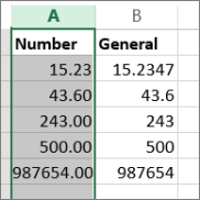
Works very much like the General format but varies how it shows numbers with decimal place separators and negative numbers. Here are some examples of how both formats display numbers:
Shows a monetary symbol with numbers. You can specify the number of decimal places with Increase Decimal or Decrease Decimal.
Also used for monetary values, but aligns the currency symbols and decimal points of numbers in a column.
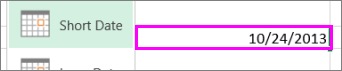
Shows date in this format:
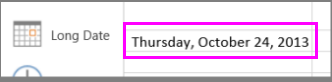
Shows month, day and year in this format:
Shows number date and time serial numbers as time values.
Multiplies the cell value by 100 and displays the result with a percent ( %) symbol.
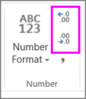
Use Increase Decimal or Decrease Decimal to specify the number of decimal places you want.
Shows the number as a fraction. For example, 0.5 displays as ½.
Displays numbers in exponential notation, replacing part of the number with E+ n, where E (Exponent) multiplies the preceding number by 10 to the nth power. For example, a 2-decimal Scientific format displays 12345678901 as 1.23E+10, which is 1.23 times 10 to the 10th power. To specify the number of decimal places you want to use, apply Increase Decimal or Decrease Decimal.
Treats the cell value as text and displays it exactly as you type it, even when you type numbers. Learn more about formatting numbers as text.
Need more help?
You can always ask an expert in the Excel Tech Community or get support in the Answers community.
Источник
Add numbers in Excel 2013
You can use Excel to add numbers using formulas, buttons, and functions.
Want more?
You can use Excel to add numbers using formulas, buttons, and functions.
Let’s take a look.
You add numbers in cells by using formulas.
A formula always starts with the equals sign. I then enter a number, then a plus sign, then another number, and press Enter.
And the cell displays the results.
You can add many numbers this way, not just two.
Instead of adding numbers within a cell, you can also reference cells to make adding a bit easier.
B2 is equal to 6, B3 is equal to 3
I’ll create a formula that adds the cells.
I start with an equals sign, click a cell that I want to add, then a plus sign, and then another cell, and press Enter.
If I change a number in a cell, the results automatically update.
You can also add many cells this way, not just two.
You can even add cells and numbers.
I start with the equals sign, click a cell I want to add, then a plus sign, then another cell, then another plus sign, the number, and press Enter.
When you double-click a cell, you can see if it has a number or a formula, or you can look up here in the Formula Bar.
AutoSum makes it easy to add adjacent cells in rows and columns.
Click the cell below a column of adjacent cells or to the right of a row of adjacent cells.
Then, on the HOME tab, click AutoSum, and press Enter.
Excel adds all of the cells in the column or row. It’s really handy.
The keyboard shortcut for AutoSum is Alt + =.
You can even select an adjacent group of cells and an extra column and row. Click AutoSum and you get the sum for each row and column, and a grand total.
AutoSum has a number of options.
Choose an option, such as Average, and Excel calculates the average for the row.
To copy a cell and its formula, click the cell, click the bottom right of the cell border so that you see a plus sign, hold down your left mouse button and drag it to the right for a column or down for a row.
And the formula is copied into the new cells.
Источник
Convert numbers stored as text to numbers
Numbers that are stored as text can cause unexpected results, like an uncalculated formula showing instead of a result. Most of the time, Excel will recognize this and you’ll see an alert next to the cell where numbers are being stored as text. If you see the alert, select the cells, and then click  to choose a convert option.
Check out Format numbers to learn more about formatting numbers and text in Excel.

If the alert button is not available, do the following:
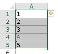
1. Select a column
Select a column with this problem. If you don’t want to convert the whole column, you can select one or more cells instead. Just be sure the cells you select are in the same column, otherwise this process won’t work. (See «Other ways to convert» below if you have this problem in more than one column.)
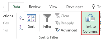
2. Click this button
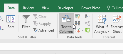
The Text to Columns button is typically used for splitting a column, but it can also be used to convert a single column of text to numbers. On the Data tab, click Text to Columns.
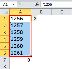
3. Click Apply
The rest of the Text to Columns wizard steps are best for splitting a column. Since you’re just converting text in a column, you can click Finish right away, and Excel will convert the cells.
4. Set the format

Press CTRL + 1 (or  + 1 on the Mac). Then select any format.
Note: If you still see formulas that are not showing as numeric results, then you may have Show Formulas turned on. Go to the Formulas tab and make sure Show Formulas is turned off.
Other ways to convert:
You can use the VALUE function to return just the numeric value of the text.
1. Insert a new column
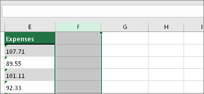
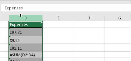
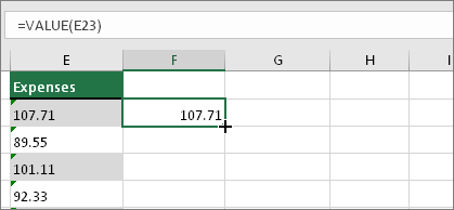
Insert a new column next to the cells with text. In this example, column E contains the text stored as numbers. Column F is the new column.
2. Use the VALUE function
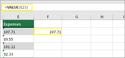
In one of the cells of the new column, type =VALUE() and inside the parentheses, type a cell reference that contains text stored as numbers. In this example it’s cell E23.
3. Rest your cursor here
Now you’ll fill the cell’s formula down, into the other cells. If you’ve never done this before, here’s how to do it: Rest your cursor on the lower-right corner of the cell until it changes to a plus sign.
4. Click and drag down
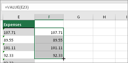
Click and drag down to fill the formula to the other cells. After that’s done, you can use this new column, or you can copy and paste these new values to the original column. Here’s how to do that: Select the cells with the new formula. Press CTRL + C. Click the first cell of the original column. Then on the Home tab, click the arrow below Paste, and then click Paste Special > Values.
If the steps above didn’t work, you can use this method, which can be used if you’re trying to convert more than one column of text.
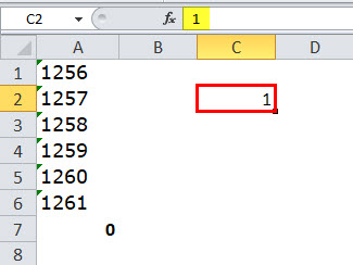
Select a blank cell that doesn’t have this problem, type the number 1 into it, and then press Enter.
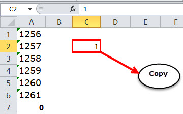
Press CTRL + C to copy the cell.
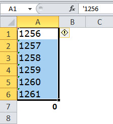
Select the cells that have numbers stored as text.
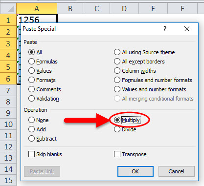
On the Home tab, click Paste > Paste Special.
Click Multiply, and then click OK. Excel multiplies each cell by 1, and in doing so, converts the text to numbers.
Press CTRL + 1 (or + 1 on the Mac). Then select any format.
Источник
Custom Excel number format
 by Svetlana Cheusheva, updated on March 20, 2023
This tutorial explains the basics of the Excel number format and provides the detailed guidance to create custom formatting. You will learn how to show the required number of decimal places, change alignment or font color, display a currency symbol, round numbers by thousands, show leading zeros, and much more.
Microsoft Excel has a lot of built-in formats for number, currency, percentage, accounting, dates and times. But there are situations when you need something very specific. If none of the inbuilt Excel formats meets your needs, you can create your own number format.
Number formatting in Excel is a very powerful tool, and once you learn how to use it property, your options are almost unlimited. The aim of this tutorial is to explain the most essential aspects of Excel number format and set you on the right track to mastering custom number formatting.
How to create a custom number format in Excel
To create a custom Excel format, open the workbook in which you want to apply and store your format, and follow these steps:
- Select a cell for which you want to create custom formatting, and press Ctrl+1 to open the Format Cells dialog.
- Under Category, select Custom.
- Type the format code in the Type box.
- Click OK to save the newly created format.
Done! 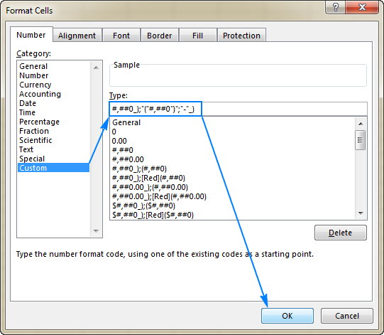
Tip. Instead of creating a custom number format from scratch, you choose a built-in Excel format close to your desired result, and customize it.
Wait, wait, but what do all those symbols in the Type box mean? And how do I put them in the right combination to display the numbers the way I want? Well, this is what the rest of this tutorial is all about 🙂
Understanding Excel number format
To be able to create a custom format in Excel, it is important that you understand how Microsoft Excel sees the number format.
An Excel number format consists of 4 sections of code, separated by semicolons, in this order:
POSITIVE; NEGATIVE; ZERO; TEXT
Here’s an example of a custom Excel format code: 
- Format for positive numbers (display 2 decimal places and a thousands separator).
- Format for negative numbers (the same as for positive numbers, but enclosed in parentheses).
- Format for zeros (display dashes instead of zeros).
- Format for text values (display text in magenta font color).
Excel formatting rules
When creating a custom number format in Excel, please remember these rules:
- A custom Excel number format changes only the visual representation, i.e. how a value is displayed in a cell. The underlying value stored in a cell is not changed.
- When you are customizing a built-in Excel format, a copy of that format is created. The original number format cannot be changed or deleted.
- Excel custom number format does not have to include all four sections.
If a custom format contains just 1 section, that format will be applied to all number types — positive, negative and zeros.
If a custom number format includes 2 sections, the first section is used for positive numbers and zeros, and the second section — for negative numbers.
A custom format is applied to text values only if it contains all four sections.
To apply the default Excel number format for any of the middle sections, type General instead of the corresponding format code.
For example, to display zeros as dashes and show all other values with the default formatting, use this format code: General; -General; «-«; General
Note. The General format included in the 2 nd section of the format code does not display the minus sign, therefore we include it in the format code.
For example, to hide zeros and negative values, use the following format code: General; ; ; General . As the result, zeros and negative value will appear only in the formula bar, but will not be visible in cells.
Digit and text placeholders
For starters, let’s learn 4 basic placeholders that you can use in your custom Excel format.
| Code | Description | Example |
| 0 | Digit placeholder that displays insignificant zeros. | #.00 — always displays 2 decimal places.
If you type 5.5 in a cell, it will display as 5.50. |
| # | Digit placeholder that only displays significant digits, without extra zeros.
That is, if a number doesn’t need a certain digit, it won’t be displayed. |
#.## — displays up to 2 decimal places.
If you type 5.5 in a cell, it will display as 5.5. If you type 5.555, it will display as 5.56. |
| ? | Digit placeholder that leaves a space for insignificant zeros on either side of the decimal point but doesn’t display them. It is often used to align numbers in a column by decimal point. | #. — displays a maximum of 3 decimal places and aligns numbers in a column by decimal point. |
| @ | Text placeholder | 0.00; -0.00; 0; [Red]@ — applies the red font color for text values. |
The following screenshot demonstrates a few number formats in action: 
As you may have noticed in the above screenshot, the digit placeholders behave in the following way:
- If a number entered in a cell has more digits to the right of the decimal point than there are placeholders in the format, the number is «rounded» to as many decimal places as there are placeholders.
For example, if you type 2.25 in a cell with #.# format, the number will display as 2.3.
All digits to the left of the decimal point are displayed regardless of the number of placeholders.
For example, if you type 202.25 in a cell with #.# format, the number will display as 202.3.
Below you will find a few more examples that will hopefully shed more light on number formatting in Excel.
| Format | Description | Input value | Display as |
| #.00 | Always display 2 decimal places. | 2 2.5 0.5556 |
2.00 2.50 .56 |
| #.## | Shows up to 2 decimal places, without insignificant zeros. | 2 2.5 0.5556 |
2. 2.5 0.56 |
| #.0# | Display a minimum of 1 and a maximum of 2 decimal places. | 2 2.205 0.555 |
2.0 2.21 .56 |
| . | Display up to 3 decimal places with aligned decimals. | 22.55 2.5 2222.5555 0.55 |
22.55 2.5 2222.556 .55 |
Excel formatting tips and guidelines
Theoretically, there are an infinite number of Excel custom number formats that you can make using a predefined set of formatting codes listed in the table below. And the following tips explain the most common and useful implementations of these format codes.
| Format Code | Description |
| General | General number format |
| # | Digit placeholder that represents optional digits and does not display extra zeros. |
| 0 | Digit placeholder that displays insignificant zeros. |
| ? | Digit placeholder that leaves a space for insignificant zeros but doesn’t display them. |
| @ | Text placeholder |
| . (period) | Decimal point |
| , (comma) | Thousands separator. A comma that follows a digit placeholder scales the number by a thousand. |
| Displays the character that follows it. | |
| » « | Display any text enclosed in double quotes. |
| % | Multiplies the numbers entered in a cell by 100 and displays the percentage sign. |
| / | Represents decimal numbers as fractions. |
| E | Scientific notation format |
| _ (underscore) | Skips the width of the next character. It’s commonly used in combination with parentheses to add left and right indents, _( and _) respectively. |
| * (asterisk) | Repeats the character that follows it until the width of the cell is filled. It’s often used in combination with the space character to change alignment. |
| [] | Create conditional formats. |
How to control the number of decimal places
The location of the decimal point in the number format code is represented by a period (.). The required number of decimal places is defined by zeros (0). For example:
- 0 or # — display the nearest integer with no decimal places.
- 0.0 or #.0 — display 1 decimal place.
- 0.00 or #.00 — display 2 decimal places, etc.
The difference between 0 and # in the integer part of the format code is as follows. If the format code has only pound signs (#) to the left of the decimal point, numbers less than 1 begin with a decimal point. For example, if you type 0.25 in a cell with #.00 format, the number will display as .25. If you use 0.00 format, the number will display as 0.25. 
How to show a thousands separator
To create an Excel custom number format with a thousands separator, include a comma (,) in the format code. For example:
- #,### — display a thousands separator and no decimal places.
- #,##0.00 — display a thousands separator and 2 decimal places.

Round numbers by thousand, million, etc.
As demonstrated in the previous tip, Microsoft Excel separates thousands by commas if a comma is enclosed by any digit placeholders — pound sign (#), question mark (?) or zero (0). If no digit placeholder follows a comma, it scales the number by thousand, two consecutive commas scale the number by million, and so on.
For example, if a cell format is #.00, and you type 5000 in that cell, the number 5.00 is displayed. For more examples, please see the screenshot below: 
Text and spacing in custom Excel number format
To display both text and numbers in a cell, do the following:
- To add a single character, precede that character with a backslash ().
- To add a text string, enclose it in double quotation marks (» «).
For example, to indicate that numbers are rounded by thousands and millions, you can add K and M to the format codes, respectively:
- To display thousands: #.00,K
- To display millions: #.00,,M
Tip. To make the number format better readable, include a space between a comma and backward slash.
The following screenshot shows the above formats and a couple more variations: 
And here is another example that demonstrates how to display text and numbers within a single cell. Supposing, you want to add the word «Increase» for positive numbers, and «Decrease» for negative numbers. All you have to do is include the text enclosed in double quotes in the appropriate section of your format code:
#.00″ Increase»; -#.00″ Decrease»; 0
Tip. To include a space between a number and text, type a space character after the opening or before the closing quote depending on whether the text precedes or follows the number, like in «Increase «. 
In addition, the following characters can be included in Excel custom format codes without the use of backslash or quotation marks:
| Symbol | Description |
| + and — | Plus and minus signs |
| ( ) | Left and right parentheses |
| : | Colon |
| ^ | Caret |
| ‘ | Apostrophe |
| Curly brackets | |
| Less-than and greater than signs | |
| = | Equal sign |
| / | Forward slash |
| ! | Exclamation point |
| & | Ampersand |
| Tilde | |
| Space character |
A custom Excel number format can also accept other special symbols such as currency, copyright, trademark, etc. These characters can be entered by typing their four-digit ANSI codes while holding down the ALT key. Here are some of the most useful ones:
| Symbol | Code | Description |
| в„ў | Alt+0153 | Trademark |
| В© | Alt+0169 | Copyright symbol |
| В° | Alt+0176 | Degree symbol |
| В± | Alt+0177 | Plus-Minus sign |
| Вµ | Alt+0181 | Micro sign |
For example, to display temperatures, you can use the format code #»В°F» or #»В°C» and the result will look similar to this: 
You can also create a custom Excel format that combines some specific text and the text typed in a cell. To do this, enter the additional text enclosed in double quotes in the 4 th section of the format code before or after the text placeholder (@), or both.
For example, to proceed the text typed in the cell with some other text, say «Shipped in«, use the following format code:
General; General; General; «Shipped in «@ 
Including currency symbols in a custom number format
To create a custom number format with the dollar sign ($), simply type it in the format code where appropriate. For example, the format $#.00 will display 5 as $5.00.
Other currency symbols are not available on most of standard keyboards. But you can enter the popular currencies in this way:
- Turn NUM LOCK on, and
- Use the numeric keypad to type the ANSI code for the currency symbol you want to display.
| Symbol | Currency | Code |
| € | Euro | ALT+0128 |
| ВЈ | British Pound | ALT+0163 |
| ВҐ | Japanese Yen | ALT+0165 |
| Вў | Cent Sign | ALT+0162 |
The resulting number formats may look something similar to this: 
If you want to create a custom Excel format with some other currency, follow these steps:
How to display leading zeros with Excel custom format
If you try entering numbers 005 or 00025 in a cell with the default General format, you would notice that Microsoft Excel removes leading zeros because the number 005 is same as 5. But sometimes, we do want 005, not 5!
The simplest solution is to apply the Text format to such cells. Alternatively, you can type an apostrophe (‘) in front of the numbers. Either way, Excel will understand that you want any cell value to be treated as a text string. As the result, when you type 005, all leading zeros will be preserved, and the number will show up as 005.
If you want all numbers in a column to contain a certain number of digits, with leading zeros if needed, then create a custom format that includes only zeros.
As you remember, in Excel number format, 0 is the placeholder that displays insignificant zeros. So, if you need numbers consisting of 6 digits, use the following format code: 000000
And now, if you type 5 in a cell, it will appear as 000005; 50 will appear as 000050, and so on: 
Tip. If you are entering phone numbers, zip codes, or social security numbers that contain leading zeros, the easiest way is to apply one of the predefined Special formats. Or, you can create the desired custom number format. For example, to properly display international seven-digit postal codes, use this format: 0000000. For social security numbers with leading zeros, apply this format: 000-00-0000.
Percentages in Excel custom number format
To display a number as a percentage of 100, include the percent sign (%) in your number format.
For example, to display percentages as integers, use this format: #%. As the result, the number 0.25 entered in a cell will appear as 25%.
To display percentages with 2 decimal places, use this format: #.00%
To display percentages with 2 decimal places and a thousands separator, use this one: #,##.00% 
Fractions in Excel number format
Fractions are special in terms that the same number can be displayed in a variety of ways. For example, 1.25 can be shown as 1 Вј or 5/5. Exactly which way Excel displays the fraction is determined by the format codes that you use.
For decimal numbers to appear as fractions, include forward slash (/) in your format code, and separate an integer part with a space. For example:
- # #/# — displays a fraction remainder with up to 1 digit.
- # ##/## — displays a fraction remainder with up to 2 digits.
- # ###/### — displays a fraction remainder with up to 3 digits.
- ###/### — displays an improper fraction (a fraction whose numerator is larger than or equal to the denominator) with up to 3 digits.
To round fractions to a specific denominator, supply it in your number format code after the slash. For example, to display decimal numbers as eighths, use the following fixed base fraction format: # #/8
The following screenshot demonstrated the above format codes in action: 
As you probably know, the predefined Excel Fraction formats align numbers by the fraction bar (/) and display the whole number at some distance from the remainder. To implement this alignment in your custom format, use the question mark placeholders (?) instead of the pound signs (#) like shown in the following screenshot: 
Tip. To enter a fraction in a cell formatted as General, preface the fraction with a zero and a space. For instance, to enter 4/8 in a cell, you type 0 4/8. If you type 4/8, Excel will assume you are entering a date, and change the cell format accordingly.
Create a custom Scientific Notation format
To display numbers in Scientific Notation format (Exponential format), include the capital letter E in your number format code. For example:
- 00E+00 — displays 1,500,500 as 1.50E+06.
- #0.0E+0 — displays 1,500,500 as 1.5E+6
- #E+# — displays 1,500,500 as 2E+6

Show negative numbers in parentheses
At the beginning of this tutorial, we discussed the 4 code sections that make up an Excel number format: Positive; Negative; Zero; Text
Most of the format codes we’ve discussed so far contained just 1 section, meaning that the custom format is applied to all number types — positive, negative and zeros.
To make a custom format for negative numbers, you’d need to include at least 2 code sections: the first will be used for positive numbers and zeros, and the second — for negative numbers.
To show negative values in parentheses, simply include them in the second section of your format code, for example: #.00; (#.00)
Tip. To line up positive and negative numbers at the decimal point, add an indent to the positive values section, e.g. 0.00_); (0.00)

Display zeroes as dashes or blanks
The built-in Excel Accounting format shows zeros as dashes. This can also be done in your custom Excel number format.
As you remember, the zero layout is determined by the 3 rd section of the format code. So, to force zeros to appear as dashes, type «-« in that section. For example: 0.00;(0.00);»-«
The above format code instructs Excel to display 2 decimal places for positive and negative numbers, enclose negative numbers in parentheses, and turn zeros into dashes.
If you don’t want any special formatting for positive and negative numbers, type General in the 1 st and 2 nd sections: General; -General; «-«
To turn zeroes into blanks, skip the third section in the format code, and only type the ending semicolon: General; -General; ; General 
Add indents with custom Excel format
If you don’t want the cell contents to ride up right against the cell border, you can indent information within a cell. To add an indent, use the underscore (_) to create a space equal to the width of the character that follows it.
The commonly used indent codes are as follows:
- To indent from the left border: _(
- To indent from the right border: _)
Most often, the right indent is included in a positive number format, so that Excel leaves space for the parentheses enclosing negative numbers.
For example, to indent positive numbers and zeros from the right and text from the left, you can use the following format code:
Or, you can add indents on both sides of the cell:
The indent codes move the cell data by one character width. To move values from the cell edges by more than one character width, include 2 or more consecutive indent codes in your number format. The following screenshot demonstrates indenting cell contents by 1 and 2 characters: 
Change font color with custom number format
Changing the font color for a certain value type is one of the simplest things you can do with a custom number format in Excel, which supports 8 main colors. To specify the color, just type one of the following color names in an appropriate section of your number format code.
| [Black] [Green] [White] [Blue] |
[Magenta] [Yellow] [Cyan] [Red] |
Note. The color code must be the first item in the section.
For example, to leave the default General format for all value types, and change only the font color, use the format code similar to this:
Or, combine color codes with the desired number formatting, e.g. display the currency symbol, 2 decimal places, a thousands separator, and show zeros as dashes:
[Blue]$#,##0.00; [Red]-$#,##0.00; [Black]»-«; [Magenta]@ 
Repeat characters with custom format codes
To repeat a specific character in your custom Excel format so that it fills the column width, type an asterisk (*) before the character.
For example, to include enough equality signs after a number to fill the cell, use this number format: #*=
Or, you can include leading zeros by adding *0 before any number format, e.g. *0# 
This formatting technique is commonly used to change cell alignment as demonstrated in the next formatting tip.
How to change alignment in Excel with custom number format
A usual way to change alignment in Excel is using the Alignment tab on the ribbon. However, you can «hardcode» cell alignment in a custom number format if needed.
For example, to align numbers left in a cell, type an asterisk and a space after the number code, for example: «#,###* » (double quotes are used only to show that an asterisk is followed by a space, you don’t need them in a real format code).
Making a step further, you could have numbers aligned left and text entries aligned right using this custom format:
#,###* ; -#,###* ; 0* ;* @ 
This method is used in the built-in Excel Accounting format . If you apply the Accounting format to some cell, then open the Format Cells dialog, switch to the Custom category and look at the Type box, you will see this format code:
The asterisk that follows the currency sign tells Excel to repeat the subsequent space character until the width of a cell is filled. This is why the Accounting number format aligns the currency symbol to the left, number to the right, and adds as many spaces as necessary in between.
Apply custom number formats based on conditions
To have your custom Excel format applied only if a number meets a certain condition, type the condition consisting of a comparison operator and a value, and enclose it in square brackets [].
For example, to displays numbers that are less than 10 in a red font color, and numbers that are greater than or equal to 10 in a green color, use this format code:
Additionally, you can specify the desired number format, e.g. show 2 decimal places:
[Red][ =10]0.00 
And here is another extremely useful, though rarely used formatting tip. If a cell displays both numbers and text, you can make a conditional format to show a noun in a singular or plural form depending on the number. For example:
The above format code works as follows:
- If a cell value is equal to 1, it will display as «1 mile«.
- If a cell value is greater than 1, the plural form «miles» will show up. Say, the number 3.5 will display as «3.5 miles«.
Taking the example further, you can display fractions instead of decimals:
In this case, the value 3.5 will appear as «3 1/2 miles«. 
Tip. To apply more sophisticated conditions, use Excel’s Conditional Formatting feature, which is specially designed to handle the task.
Dates and times formats in Excel
Excel date and times formats are a very specific case, and they have their own format codes. For the detailed information and examples, please check out the following tutorials:
Well, this is how you can change number format in Excel and create your own formatting. Finally, here’s a couple of tips to quickly apply your custom formats to other cells and workbooks:
- A custom Excel format is stored in the workbook in which it is created and is not available in any other workbook. To use a custom format in a new workbook, you can save the current file as a template, and then use it as the basis for a new workbook.
- To apply a custom format to other cells in a click, save it as an Excel style — just select any cell with the required format, go to the Home tab >Styles group, and click New Cell Style….
To explore the formatting tips further, you can download a copy of the Excel Custom Number Format workbook we used in this tutorial. I thank you for reading and hope to see you again next week!
Источник
It’s common to find numbers stored as text in Excel. This leads to incorrect calculations when you use these cells in Excel functions such as SUM and AVERAGE (as these functions ignore cells that have text values in it). In such cases, you need to convert cells that contain numbers as text back to numbers.
Now before we move forward, let’s first look at a few reasons why you may end up with a workbook that has numbers stored as text.
- Using ‘ (apostrophe) before a number.
- A lot of people enter apostrophe before a number to make it text. Sometimes, it’s also the case when you download data from a database. While this makes the numbers show up without the apostrophe, it impacts the cell by forcing it to treat the numbers as text.
- Getting numbers as a result of a formula (such as LEFT, RIGHT, or MID)
- If you extract the numerical part of a text string (or even a part of a number) using the TEXT functions, the result is a number in the text format.
Now, let’s see how to tackle such cases.
Convert Text to Numbers in Excel
In this tutorial, you’ll learn how to convert text to numbers in Excel.
The method you need to use depends on how the number has been converted into text. Here are the ones that are covered in this tutorial.
- Using the ‘Convert to Number’ option.
- Change the format from Text to General/Number.
- Using Paste Special.
- Using Text to Columns.
- Using a Combination of VALUE, TRIM, and CLEAN function.
Convert Text to Numbers Using ‘Convert to Number’ Option
When an apostrophe is added to a number, it changes the number format to text format. In such cases, you’ll notice that there is a green triangle at the top left part of the cell.
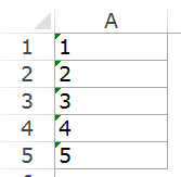
In this case, you can easily convert numbers to text by following these steps:
- Select all the cells that you want to convert from text to numbers.

- Click on the yellow diamond shape icon that appears at the top right. From the menu that appears, select ‘Convert to Number’ option.
This would instantly convert all the numbers stored as text back to numbers. You would notice that the numbers get aligned to the right after the conversion (while these were aligned to the left when stored as text).
Convert Text to Numbers by Changing Cell Format
When the numbers are formatted as text, you can easily convert it back to numbers by changing the format of the cells.
Here are the steps:
- Select all the cells that you want to convert from text to numbers.
- Go to Home –> Number. In the Number Format drop-down, select General.
This would instantly change the format of the selected cells to General and the numbers would get aligned to the right. If you want, you can select any of the other formats (such as Number, Currency, Accounting) which will also lead to the value in cells being considered as numbers.
Also read: How to Convert Serial Numbers to Dates in Excel
Convert Text to Numbers Using Paste Special Option
To convert text to numbers using Paste Special option:
Convert Text to Numbers Using Text to Column
This method is suitable in cases where you have the data in a single column.
Here are the steps:
- Select all the cells that you want to convert from text to numbers.
- Go to Data –> Data Tools –> Text to Columns.

- In the Text to Column Wizard:
While you may still find the resulting cells to be in the text format, and the numbers still aligned to the left, now it would work in functions such as SUM and AVERAGE.
Convert Text to Numbers Using the VALUE Function
You can use a combination of VALUE, TRIM and CLEAN function to convert text to numbers.
- VALUE function converts any text that represents a number back to a number.
- TRIM function removes any leading or trailing spaces.
- CLEAN function removes extra spaces and non-printing characters that might sneak in if you import the data or download from a database.
Suppose you want convert cell A1 from text to numbers, here is the formula:
=VALUE(TRIM(CLEAN(A1)))
If you want to apply this to other cells as well, you can copy and use the formula.
Finally, you can convert the formula to value using paste special.
You May Also Like the Following Excel Tutorials:
- Multiply in Excel Using Paste Special.
- How to Convert Text to Date in Excel (8 Easy Ways)
- How to Convert Numbers to Text in Excel
- Convert Formula to Values Using Paste Special.
- Excel Custom Number Formatting.
- Convert Time to Decimal Number in Excel
- Change Negative Number to Positive in Excel
- How to Capitalize First Letter of a Text String in Excel
- Convert Scientific Notation to Number or Text in Excel
- How To Convert Date To Serial Number In Excel?
Introduction
Number formats control how numbers are displayed in Excel. The key benefit of number formats is that they change how a number looks without changing any data. They are a great way to save time in Excel because they perform a huge amount of formatting automatically. As a bonus, they make worksheets look more consistent and professional.
Video: What is a number format
What can you do with custom number formats?
Custom number formats can control the display of numbers, dates, times, fractions, percentages, and other numeric values. Using custom formats, you can do things like format dates to show month names only, format large numbers in millions or thousands, and display negative numbers in red.

Where can you use custom number formats?
Many areas in Excel support number formats. You can use them in tables, charts, pivot tables, formulas, and directly on the worksheet.
- Worksheet — format cells dialog
- Pivot Tables — via value field settings
- Charts — data labels and axis options
- Formulas — via the TEXT function
What is a number format?
A number format is a special code to control how a value is displayed in Excel. For example, the table below shows 7 different number formats applied to the same date, January 1, 2019:
| Input | Code | Result |
|---|---|---|
| 1-Jan-2019 | yyyy | 2019 |
| 1-Jan-2019 | yy | 19 |
| 1-Jan-2019 | mmm | Jan |
| 1-Jan-2019 | mmmm | January |
| 1-Jan-2019 | d | 1 |
| 1-Jan-2019 | ddd | Tue |
| 1-Jan-2019 | dddd | Tuesday |
The key thing to understand is that number formats change the way numeric values are displayed, but they do not change the actual values.
Where can you find number formats?
On the home tab of the ribbon, you’ll find a menu of build-in number formats. Below this menu to the right, there is a small button to access all number formats, including custom formats:

This button opens the Format Cells dialog box. You’ll find a complete list of number formats, organized by category, on the Number tab:

Note: you can open Format Cells dialog box with the keyboard shortcut Control + 1.
General is default
By default, cells start with the General format applied. The display of numbers using the General number format is somewhat «fluid». Excel will display as many decimal places as space allows, and will round decimals and use scientific number format when space is limited. The screen below shows the same values in column B and D, but D is narrower and Excel makes adjustments on the fly.

How to change number formats
You can select standard number formats (General, Number, Currency, Accounting, Short Date, Long Date, Time, Percentage, Fraction, Scientific, Text) on the home tab of the ribbon using the Number Format menu.
Note: As you enter data, Excel will sometimes change number formats automatically. For example if you enter a valid date, Excel will change to «Date» format. If you enter a percentage like 5%, Excel will change to Percentage, and so on.
Shortcuts for number formats
Excel provides a number of keyboard shortcuts for some common formats:
| Format | Shortcut |
|---|---|
| General format | Ctrl Shift ~ |
| Currency format | Ctrl Shift $ |
| Percentage format | Ctrl Shift % |
| Scientific format | Ctrl Shift ^ |
| Date format | Ctrl Shift # |
| Time format | Ctrl Shift @ |
| Custom formats | Control + 1 |
See also: 222 Excel Shortcuts for Windows and Mac
Where to enter custom formats
At the bottom of the predefined formats, you’ll see a category called custom. The Custom category shows a list of codes you can use for custom number formats, along with an input area to enter codes manually in various combinations.

When you select a code from the list, you’ll see it appear in the Type input box. Here you can modify existing custom code, or to enter your own codes from scratch. Excel will show a small preview of the code applied to the first selected value above the input area.
Note: Custom number formats live in a workbook, not in Excel generally. If you copy a value formatted with a custom format from one workbook to another, the custom number format will be transferred into the workbook along with the value.
How to create a custom number format
To create custom number format follow this simple 4-step process:
- Select cell(s) with values you want to format
- Control + 1 > Numbers > Custom
- Enter codes and watch preview area to see result
- Press OK to save and apply
Tip: if you want base your custom format on an existing format, first apply the base format, then click the «Custom» category and edit codes as you like.
How to edit a custom number format
You can’t really edit a custom number format per se. When you change an existing custom number format, a new format is created and will appear in the list in the Custom category. You can use the Delete button to delete custom formats you no longer need.
Warning: there is no «undo» after deleting a custom number format!
Structure and Reference
Excel custom number formats have a specific structure. Each number format can have up to four sections, separated with semi-colons as follows:

This structure can make custom number formats look overwhelmingly complex. To read a custom number format, learn to spot the semi-colons and mentally parse the code into these sections:
- Positive values
- Negative values
- Zero values
- Text values
Not all sections required
Although a number format can include up to four sections, only one section is required. By default, the first section applies to positive numbers, the second section applies to negative numbers, the third section applies to zero values, and the fourth section applies to text.
- When only one format is provided, Excel will use that format for all values.
- If you provide a number format with just two sections, the first section is used for positive numbers and zeros, and the second section is used for negative numbers.
- To skip a section, include a semi-colon in the proper location, but don’t specify a format code.
Characters that display natively
Some characters appear normally in a number format, while others require special handling. The following characters can be used without any special handling:
| Character | Comment |
|---|---|
| $ | Dollar |
| +- | Plus, minus |
| () | Parentheses |
| {} | Curly braces |
| <> | Less than, greater than |
| = | Equal |
| : | Colon |
| ^ | Caret |
| ‘ | Apostrophe |
| / | Forward slash |
| ! | Exclamation point |
| & | Ampersand |
| ~ | Tilde |
| Space character |
Escaping characters
Some characters won’t work correctly in a custom number format without being escaped. For example, the asterisk (*), hash (#), and percent (%) characters can’t be used directly in a custom number format – they won’t appear in the result. The escape character in custom number formats is the backslash (). By placing the backslash before the character, you can use them in custom number formats:
| Value | Code | Result |
|---|---|---|
| 100 | #0 | #100 |
| 100 | *0 | *100 |
| 100 | %0 | %100 |
Placeholders
Certain characters have special meaning in custom number format codes. The following characters are key building blocks:
| Character | Purpose |
|---|---|
| 0 | Display insignificant zeros |
| # | Display significant digits |
| ? | Display aligned decimals |
| . | Decimal point |
| , | Thousands separator |
| * | Repeat following character |
| _ | Add space |
| @ | Placeholder for text |
Zero (0) is used to force the display of insignificant zeros when a number has fewer digits than zeros in the format. For example, the custom format 0.00 will display zero as 0.00, 1.1 as 1.10 and .5 as 0.50.

Pound sign (#) is a placeholder for optional digits. When a number has fewer digits than # symbols in the format, nothing will be displayed. For example, the custom format #.## will display 1.15 as 1.15 and 1.1 as 1.1.

Question mark (?) is used to align digits. When a question mark occupies a place not needed in a number, a space will be added to maintain visual alignment.

Period (.) is a placeholder for the decimal point in a number. When a period is used in a custom number format, it will always be displayed, regardless of whether the number contains decimal values.
Comma (,) is a placeholder for the thousands separators in the number being displayed. It can be used to define the behavior of digits in relation to the thousands or millions digits.

Asterisk (*) is used to repeat characters. The character immediately following an asterisk will be repeated to fill remaining space in a cell.

Underscore (_) is used to add space in a number format. The character immediately following an underscore character controls how much space to add. A common use of the underscore character is to add space to align positive and negative values when a number format is adding parentheses to negative numbers only. For example, the number format «0_);(0)» is adding a bit of space to the right of positive numbers so that they stay aligned with negative numbers, which are enclosed in parentheses.

At (@) — placeholder for text. For example, the following number format will display text values in blue:
0;0;0;[Blue]@
See below for more information about using color.
Automatic rounding
It’s important to understand that Excel will perform «visual rounding» with all custom number formats. When a number has more digits than placeholders on the right side of the decimal point, the number is rounded to the number of placeholders. When a number has more digits than placeholders on the left side of the decimal point, extra digits are displayed. This is a visual effect only; actual values are not modified.
Number formats for TEXT
To display both text along with numbers, enclose the text in double quotes («»). You can use this approach to append or prepend text strings in a custom number format, as shown in the table below.
| Value | Code | Result |
|---|---|---|
| 10 | General» units» | 10 units |
| 10 | 0.0″ units» | 10.0 units |
| 5.5 | 0.0″ feet» | 5.5 feet |
| 30000 | 0″ feet» | 30000 feet |
| 95.2 | «Score: «0.0 | Score: 95.2 |
| 1-Jun | «Date: «mmmm d | Date: June 1 |
Number formats for DATES
Dates in Excel are just numbers, so you can use custom number formats to change the way they display. Excel has many specific codes you can use to display components of a date in different ways. The screen below shows how Excel displays the date in D5, September 3, 2018, with a variety of custom number formats:

Number formats for TIME
Times in Excel are fractional parts of a day. For example, 12:00 PM is 0.5, and 6:00 PM is 0.75. You can use the following codes in custom time formats to display components of a time in different ways. The screen below shows how Excel displays the time in D5, 9:35:07 AM, with a variety of custom number formats:

Note: m and mm can’t be used alone in a custom number format since they conflict with the month number code in date format codes.
Number formats for ELAPSED TIME
Elapsed time is a special case and needs special handling. By using square brackets, Excel provides a special way to display elapsed hours, minutes, and seconds. The following screen shows how Excel displays elapsed time based on the value in D5, which represents 1.25 days:

Number formats for COLORS
Excel provides basic support for colors in custom number formats. The following 8 colors can be specified by name in a number format: [black] [white] [red][green] [blue] [yellow] [magenta] [cyan]. Color names must appear in brackets.

Colors by index
In addition to color names, it’s also possible to specify colors by an index number (Color1,Color2,Color3, etc.) The examples below are using the custom number format: [ColorX]0″▲▼», where X is a number between 1-56:
[Color1]0"▲▼" // black
[Color2]0"▲▼" // white
[Color3]0"▲▼" // red
[Color4]0"▲▼" // green
etc.
The triangle symbols have been added only to make the colors easier to see. The first image shows all 56 colors on a standard white background. The second image shows the same colors on a gray background. Note the first 8 colors shown correspond to the named color list above.


Apply number formats in a formula
Although most number formats are applied directly to cells in a worksheet, you can also apply number formats inside a formula with the TEXT function. For example, with a valid date in A1, the following formula will display the month name only:
=TEXT(A1,"mmmm")
The result of the TEXT function is always text, so you are free to concatenate the result of TEXT to other strings:
="The contract expires in "&TEXT(A1,"mmmm")
The screen below shows the number formats in column C being applied to numbers in column B using the TEXT function:

One quirk of the TEXT function relates to double quotes («») that are part of certain custom number formats. Because the format_text is entered as a text string, Excel won’t allow you to enter the formula without removing the quotes or adding more quotes. For example, to display a large number in thousands, you can use a custom number format like this:
0, "k"Notice k appears in quotes («k»). To apply the same format with the TEXT function, you can use simply:
=TEXT(A1,"0, k")Notice the k is not surrounded by quotes. Alternately, you can add extra double quotes as below, which returns the same result:
=TEXT(A1,"0,""K""")This behavior only occurs when you are hardcoding a format inside TEXT. If you are applying a format entered elsewhere on the worksheet (as in cells C6 and C9 in the worksheet above) you can use a standard number format.
Measurements
You can use a custom number format to display numbers with an inches mark («) or a feet mark (‘). In the screen below, the number formats used for inches and feet are:
0.00 ' // feet
0.00 " // inches

These results are simplistic, and can’t be combined in a single number format. You can however use a formula to display feet together with inches.
Conditionals
Custom number formats also up to two conditions, which are written in square brackets like [>100] or [<=100]. When you use conditionals in custom number formats, you override the standard [positive];[negative];[zero];[text] structure. For example, to display values below 100 in red, you can use:
[Red][<100]0;0
To display values greater than or equal to 100 in blue, you can extend the format like this:
[Red][<100]0;[Blue][>=100]0

To apply more than two conditions, or to change other cell attributes, like fill color, etc. you’ll need to switch to Conditional Formatting, which can apply formatting with much more power and flexibility using formulas.
Plural text labels
You can use conditionals to add an «s» to labels greater than zero with a custom format like this:
[=1]0″ day»;0″ days»

Telephone numbers
Custom number formats can also be used for telephone numbers, as shown in the screen below:

Notice the third and fourth examples use a conditional format to check for numbers that contain an area code. If you have data that contains phone numbers with hard-coded punctuation (parentheses, hyphens, etc.) you will need to clean the telephone numbers first so that they only contain numbers.
Hide all content
You can actually use a custom number format to hide all content in a cell. The code is simply three semi-colons and nothing else ;;;
To reveal the content again, you can use the keyboard shortcut Control + Shift + ~, which applies the General format.
Other resources
- Developer Bryan Braun built a nice interactive tool for building custom number formats
This post is going to show you all the ways you can convert text to numbers in Microsoft Excel.
An issue that comes up quite often in Excel is numbers that have been entered or formatted as text values.
This can cause many headaches when trying to troubleshoot why a formula like a SUM is not giving the correct answer.
Even though the data looks like a number, it can actually be a text value and will be ignored from any numerical calculations like a sum.
In this post, I will show you how you can identify such numbers which are stored as text values, and 7 ways you can use to convert the text into a proper number value.
How to Indentify Numbers Entered as Text
How can you tell if your number data has been entered as text?
There are quite a few easy ways to tell!
Left Aligned
The first way you might be able to tell if you have text values instead of numerical values is the way the data is aligned in the cell.
By default text is left aligned and numbers are right aligned.
Unless the alignment formatting has been changed from the default, this will be an easy way to spot numbers that have been formatted as text.
Green Triangle Error Checking
If you don’t realize you have numbers entered as text values, it can potentially cause some serious errors. This is why it’s flagged by Excel’s built-in error checker.
Any cells that are flagged with an error will show a small green triangle in the left of the cell to visually indicate an error.
When you select such a cell a small warning icon will appear.
When you click on this, it will show you what the error is. In this case, you can see the error is Number Stored as Text.
You can turn off this error checking entirely, or customize which errors are flagged.
Go to the File tab and then select Options at the bottom. This will open up the Excel Options menu.
In the Formula section of the Excel Options menu ➜ Error Checking.
Uncheck the Enable background error checking option to disable this feature. You can also customize the color used to indicate errors here.
Text Format Applied
One way that numbers get entered as text is when the cell has been formatted as text. This causes values to be entered as text values regardless of whether they are numerical.
There is a quick way to determine whether or not a cell has had text formatting applied.
Select the cell and go to the Home tab. You will be able to see if Text is the selected formatting in the dropdown menu found in the Number section of the ribbon.
Preceding Apostrophe
Another way that numbers can be entered as text is by using a preceding apostrophe.
When you enter an apostrophe ' as the first character in a cell, anything after will be regarded as a text value by Excel.
This means if you see a leading apostrophe in the formula bar, you know the data is a text value.
Use the ISTEXT Function
Excel has a function you can use to test if a value is a text value or not.
ISTEXT ( input )- input is the value, cell or range which you want to test if it is text.
The ISTEXT function will return TRUE if the value is text and FALSE otherwise.
= ISTEXT ( B3 )Here you can see the ISTEXT function being used to determine if the cells contain text. The function returns TRUE when it finds a text value.
ISNUMBER ( input )- input is the value, cell or range which you want to test if it is a number.
Similarly, you can test if a value is a number using the ISNUMBER function. It takes a single input and returns TRUE when the value is a number and FALSE otherwise.
Here the same data is tested using the ISNUMBER function. The function returns FALSE when it does not find a number.
Status Bar Only Shows a Count
Another way to quickly test a range of cells to see if they are all text is by using the status bar.
When you select a range of numerical values, Excel will show you some basic statistics like the sum, min, max, and average in the status bar.
If they are all numbers entered as text values, then these basic statistics won’t be calculated. Instead, you will only see the count of the cells in the status bar.
Note: If just one of the cells is a numerical value, you will see the full set of statistics in the status bar.
Convert Text to Number with Error Checking
You have already seen that you can use error checking to spot numbers entered as text.
The error checking will also allow you to convert these text values into proper numbers.
Click on the Error icon and choose Convert to Number from the options. Excel will then convert each cell in the selected range into a number.
Note: This option can be very slow when you have a large number of cells to convert.
Convert Text to Number with Text to Column
Usually, Text to Columns is for splitting data into multiple columns. But with this trick, you can use it to convert text format into the general format.
Text to Column will let you choose a delimiter character to split your data based on. If you deselect this option and don’t pick any delimiter then it won’t split your data.
You are then able to choose how to format the results, and this is where you can choose a general format for the output.
Follow these steps to use the text to column feature to convert text to numbers.
- Select the cells that contain the text which you want to convert into number.
- Go to the Data tab.
- Click on the Text to Column command found in the Data Tools tab.
- Select Delimited in the Original data type options.
- Press the Next button.
- Press the Next button again in step 2 of the Convert Text to Columns wizard. You can keep the default options.
- Select General from the Column data format option.
- Select a Destination if you want to place the converted values in a new location. Otherwise you can keep the default value which should be the active cell, this will replace the text with numeric values.
- Press the Finish button.
This will convert your text values into numerical values.
The Text to Column command is usually used to split comma-separated or other delimiter separated data into multiple columns.
Any delimited data will be text data, so when Excel splits the data into multiple columns it also converts numerical data into numbers for added convenience.
This is also true even if there is nothing to split!
So the Text to Column wizard can be used to converts numerical text values to numbers.
Convert Text to Number with Multiply by 1
Even when values are stored as text you can still perform certain numerical calculations with them and the results of these calculations will also be numerical values.
You can use this to convert the text into numbers by multiplying them by 1. Since you are multiplying by 1, it won’t change the numbers but it will convert them.
= B3 * 1You can use the above formula in an adjacent cell and copy and paste it down to convert an entire column.
If you want to remove the formula after, you can copy and paste them as values.
Convert Text to Number with Paste Special Multiply
Multiplying by 1 is a great trick for converting text to values, but you might not want to use a formula for this.
The great news is there is an easy way to multiply your text by 1 without using a formula.
This means you can convert your text in place and you don’t need to copy and paste formulas as values in an additional step.
You can use Paste Special Multiply to convert your text values. Follow these steps to multiply by 1 using Paste Special.
- Enter 1 into a cell elsewhere in the sheet. The 1 doesn’t even need to be a number value and can be a text value.
- Copy the cell which contains 1 using Ctrl + C on your keyboard or right click and choose Copy.
- Select the cells with the text values to convert.
- Press Ctrl + Alt + V on your keyboard or right click and choose Paste Special. This will open up the Paste Special menu.
- Select Values under the Paste options and select Multiply under the Operation options.
- Press the OK button.
This will multiply all the values by 1 which was the value in the copied cell. As a result, the text is converted into values, but since you are multiplying by 1 the numbers won’t change.
Convert Text to Number with VALUE Function
There is actually a dedicated function you can use for converting text to numerical values.
The VALUE function takes a text value and returns the text value as a number.
= VALUE ( text )- text is the text value you want to convert into a numerical value.
If the text contains any non-numerical characters, then the VALUE function will return a #VALUE! error. It doesn’t extract numbers from text, it can only convert numbers entered as text into numbers.
= VALUE ( B3 )You can use the above formula to convert the text in cell B3 into a number and then copy and paste the formula to convert the entire column.
Convert Text to Number with Power Query
Power Query is an amazing tool for any type of data transformation required. It can certainly be used to convert text into numbers as well.
Power Query is strongly typed. This means calculations with incompatible data types will result in an error. So you won’t be able to multiply text values by 1 to convert them into numbers.
But Power Query does come with an easy way to convert data types, including text to numbers.
Follow these steps once your data has been imported into Power Query.
Click on the data type icon to the left side of the column heading for the values you want to convert.
Each column in the Power Query editor has a data type icon that displays the current data type of the column. If the column has not been assigned a data type, then the icon shown will be ABC123.
There are several numeric data types available in Power Query and which one you choose will depend on the level of decimal precision you need.
In this case, you can select the Whole Number option from the menu.
Notice the values in the column are now right-aligned and the data type icon has changed? These are visual indicators that the data type is now whole numbers instead of text.
= Table.TransformColumnTypes(Source,{{"Text", Int64.Type}})You will see a new Changed Type step has been applied to the query and it will use the above M code formula.
You can then press the Close & Load button in the Home tab to save the results and load the data into Excel.
You might not even need to apply this data type conversion step to your query. When you first import data into Power Query, it will usually guess the data type and apply the conversion for you!
Convert Text to Number with Power Pivot
If you want to analyze or summarize your data after you convert it from text to numbers, then you might want to do the conversion in Power Pivot.
Power Pivot is an add-in that allows you to efficiently analyze millions of rows in the data model with Pivot Tables.
With Power Pivot, you can build row-level calculations using the DAX formula language to create new columns in your datasets. You can then access these new columns in your pivot tables connected to the data model.
In this case, the DAX formula you can use to convert text to numbers is the exact same as the formula in the grid.
Follow these steps inside the Power Pivot add-in to create a new calculated column that converts the text to numbers.
Select any cell under the Add Column heading.
=VALUE(TextNumbers[Text])Insert the above formula. TextNumbers is the name of the table of data in Power Pivot and Text is the name of the column you want to convert.
Double click on the column heading to change the name.
Press the Save icon and close the Power Pivot add-in.
Now you can create a pivot table from the data model and this new column will be available for use inside the pivot table just like any other field.
- Go to the Insert tab.
- Click on the PivotTable button.
- Choose From Data Model in the available options.
The calculated column will be available in your pivot table fields list and you will be able to use it like any other number field.
Conclusions
There are many reasons why you might have data that contains numbers formatted as text.
If you want to freely use these values in your calculations, you will need to convert them into numbers.
Thankfully, there are many easy options to convert text to numbers such as error checking, paste special, basic multiplication, and the VALUE function. These are all easy ways to convert text inside the grid.
If you’re importing your data using Power Query or Power Pivot, you can perform the conversion inside each of these tools. Both have methods available to convert text to numbers.
Do you use any of these methods to change your text values to numbers? Do you know any other interesting ways to perform this action? Let me know in the comments below!
About the Author
John is a Microsoft MVP and qualified actuary with over 15 years of experience. He has worked in a variety of industries, including insurance, ad tech, and most recently Power Platform consulting. He is a keen problem solver and has a passion for using technology to make businesses more efficient.
How to Convert Text to Numbers in Excel? (Step by Step)
There are many ways we can convert text to numbers in Excel. We will see them one by one.
- Using quick convert text to numbers Excel option.
- Use a special cell formatting method.
- Using the Text to ColumnText to columns in excel is used to separate text in different columns based on some delimited or fixed width. This is done either by using a delimiter such as a comma, space or hyphen, or using fixed defined width to separate a text in the adjacent columns.read more Method.
- Using the VALUE function.
Table of contents
- How to Convert Text to Numbers in Excel? (Step by Step)
- #1 Using quick Convert Text to Numbers Excel Option
- #2 Using Paste Special Cell Formatting Method
- #3 Using the Text to Column Method
- #4 Using the VALUE Function
- Things to Remember
- Recommended Articles
You can download this Convert Text to Numbers Excel Template here – Convert Text to Numbers Excel Template
#1 Using quick Convert Text to Numbers Excel Option
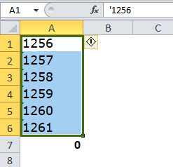
It is probably the simplest of ways in Excel. Many people use the apostrophe ( ‘ ) before entering the numbers in Excel.
Below are the steps for converting text to numbers Excel option:
- We must first select the data.

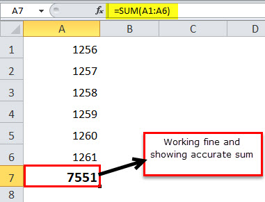
- Then, we need to click on the error handle box and select the “Convert to Number” option.

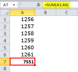
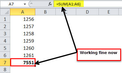
- That would instantly convert the text-formatted numbers to number format, and now the SUM function works well and shows the accurate result.


#2 Using Paste Special Cell Formatting Method
Now let us move to another way of changing the text to numbers. Here we are using the Paste Special methodPaste special in Excel allows you to paste partial aspects of the data copied. There are several ways to paste special in Excel, including right-clicking on the target cell and selecting paste special, or using a shortcut such as CTRL+ALT+V or ALT+E+S.read more. Again, consider the same data we used in the previous example.
- Step 1: First, we must type the number either zero or 1 in any one cell.
- Step 2: Now, we need to copy that number. (We have entered the number 1 in cell C2).
- Step 3: Now, we must select the numbers list.
- Step 4: Now, we must press ALT + E + S (Excel shortcut keyAn Excel shortcut is a technique of performing a manual task in a quicker way.read more for the pastespecial method). That will open up the below dialog box. Select the multiply option. (We can try to divide also).
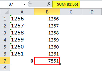
- Step 5: As a result, it would instantly convert the text to numbers, and the SUM formula is working well now.
#3 Using the Text to Column Method
It is the third method of converting text to numbers. It is a bit lengthier process than the earlier two, but it is always good to have as many alternatives as possible.
- Step 1: We must first select the data
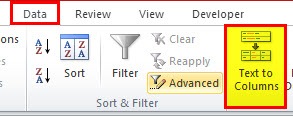
- Step 2: We need to click on the “Data” tab and the “Text to Columns” option.
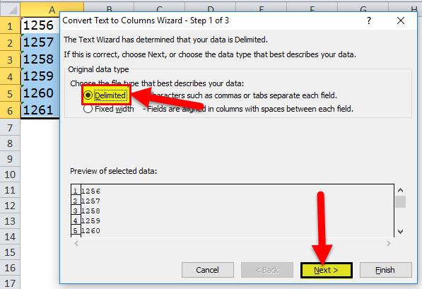
- Step 3: As a result, it will open up the below dialog box and ensure “Delimited” is selected. Click on the “Next button.”
- Step 4: We must ensure the “Tab” box is checked and click on the “Next” button.
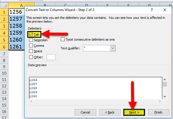
- Step 5: In the next window, we must select the “General” option, select the destination cell, and click on the “Finish” button.

- Step 6: Consequently, this would convert text to numbers, and SUM may work now.
#4 Using the VALUE Function
In addition, a formula can convert text to numbers in Excel. The VALUE function can perform the job for us. We must follow the below steps to learn how to do it.
- Step 1: First, we must apply the VALUE formula in cell B1.

- Step 2: We need to drag and drop the formula into the remaining cells.

- Step 3: Then, apply the SUM formula in cell B6 to check whether it has converted or not.
Things to Remember
- If we find the green triangle button in the cell, there must be something wrong with the data.
- The VALUE function can be useful in converting the text string that represents a number to a number.
- If spacing problems exist, we nest the VALUE function with the TRIM function. For example, =Trim(Value(A1))
- The “Text to Column” can also correct dates, numbers, and time formats.
Recommended Articles
This article is a guide to Convert Text to Numbers in Excel. Here, we discuss how to convert text to numbers in Excel using 1) Error handler, 2) text to the column, 2) PasteSpecial, and 4) Value Function and Excel examples and downloadable Excel templates. You may also look at these useful functions in Excel: –
- Convert Columns to Rows in Excel
- Convert Date to Text
- Convert Numbers to Text in Excel
- Convert Excel to CSV
Number Formatting in Excel: Step-by-Step Tutorial (2023)
We all know how to apply the basic numeric and text formats to cells in Excel.
But do you know how you can add a desired number of decimals, scientific notations, currency symbols, and similar formats in Excel with only a click?
No? This article is for you. It delves into the details of number formatting in Excel. 🤩
Keep reading till the end, and download our free sample workbook here before you scroll down.
What are number formats?
Type something into a cell. What is its format?

By default, all cells of Excel will have the General format applied.
However, type in a big number that exceeds the size of the cell, and Excel would give you back something like 1.2E+12.

What is this? A scientific notation. Under General format, Excel replaces a number too big to fit the cell with its scientific notation.
To turn it into a number, change the format to ‘Numbers’ and adjust the cell size.

Check the formula bar to note how the number remains the same under both formats i.e. 1200000000000.
What changes is only the visual representation of the said number in Excel (decimal places added).
That is how formats work in Excel.
And you can change the format of a number with a mere click. Excel offers many number formats with useful variations to them.
Thousands separator
In the image below we have different numbers.

By now, it only seems like a number that is hard to read. Maybe that’s because it doesn’t yet have 1000s separators (any commas) to it.
- Select the cell.
- Go to Home > Number

- From the menu, go to More Number Formats

This launches the Format Cells dialog box.
You may use the keyboard shortcut (Control Key + 1) to launch the Format Cells dialog box.

- Go to Number Format.
- Check the ‘Use 1000 Separator’ box.

- Here are the results.

A shortcut to add the 1000s separator: Go to Home > Number > click on the comma symbol

However, this changes the number format to the Accounting format.

Controlling decimals
In the same example, as above, there are two decimals to the number.

But you want four decimal places to this number. How can this be done?
- Select the cell.
- Go to Home > Number > More Number Formats

- From the Format Cells dialog box, go to Number Format.
- Adjust the decimal places to four.

- Here are the results.

A shortcut to adjust decimal places. Go to Home > Number > Add decimals button

With every click, Excel adds another decimal position to the number.
The button with a right-headed arrow reduces a decimal position.
The button with a left-headed arrow adds a decimal position.
Show as percentage
Here is a decimal number that we want to be converted into a percentage.

To do this:
- Select the cell.
- Go to Home > Number > More Number Formats

- From the Format Cells dialog box, go to Number Format.
- Click on Percentage.

- Adjust the decimal places as desired.

- Here are the results.

A shortcut to convert a number into a percentage. Go to Home > Number > Click the % symbol

Number formatting presets
Excel offers a wide variety of number formatting presets. (You must’ve had a slight idea of that by now.)
These range from currency to accounting to dates and whatnot.
Let’s look into each of these formats below.
General number format preset
The general number format of Excel is the default format of any value in Excel.
All values in all cells of Excel will have the general number format by default.
- To apply the general format to any cell in Excel, select that cell.
- Press the Control key + 1 to launch the Format cells dialog box. That’s a handy shortcut 😊.
- Choose the ‘General number’ format.

- Values formatted as general numbers are displayed just the way they are.
Pro Tip!
Under the General number format, if the cell is not wide enough to contain a number, Excel would:
- Round a number with decimals to lesser decimal places; or
- Use scientific notation to express the number; or
- If the cell is too small to fit in the scientific notation for the number even, display a series of hashes only.
Number format preset
The Excel number format is used for simple numeric values
To apply the number format to any cell:
- Select the cell.
- Go to Home > Numbers > Drop Down Menu and click on Number Format.

The number format allows users three further variations to the final value:
- The decimal places. You can adjust decimal places to any desired number.

- The 1000 Separator. Check the box if you need 1000s separators to the value.

- The format of negative numbers. This could be in two colors (black or red) and enclosed within brackets or with a minus sign.

The Sample box gives a preview of what the final value may look like.

Must Note:
Under the Numbers format, if you type a number in a cell that is too big to fit in the cell, Excel might return a series of hashes only.

In such a case, one must know that the problem simply lies within the size of the cell. (that is too small to fit in the cell value).
To work this out, increase the width of the column until it is wide enough to fit in the cell value.

Currency format preset
The Currency format is used to denote currencies.
To format a number as currency:
- Go to Home > Numbers > Drop Down Menu > Click on Currency.

It allows you to adjust three options to your desire:
- The decimal places.

- The currency symbol.

- The format of negative numbers. This could be in two colors (black or red) and enclosed within brackets or with a minus sign.

Here is what a currency formatted number looks like.

Date format presets
There are two date formats offered by Excel – short date and long date.

To format a number as a date, go to Format Cells and choose the date format you’d want to be applied.

Excel offers a wide variety of formats for dates and days.
Here is how the date format works.

Pro Tip!
Type any number into Excel and apply the date formatting to it. Excel turns it into a date.
This is because Excel recognizes each date as a number. Where 1 is equal to 01 Jan 1900, 2 is equal to 02 Jan 1900, and so on.
Accounting format preset
Next is the accounting format preset.
This format is relevant when you’re working with financial data. For example, while preparing financial statements, forecasts, or similar reports.
To apply accounting format to a number:
- Go to Home > Numbers > Drop Down Menu > Click on Accounting Format.

It allows you to adjust two features to your desire:
- The decimal places.

- The currency symbol.

Here is what an accounting formatted number looks like.

Under the accounting format, 1000s separators and currency symbols are added by default. And negative numbers are enclosed in parenthesis i.e. $ (1925.60) etc.
Time format preset
Excel also offers a wide variety of ways how you may represent times in Excel.
To apply the time format, go to Format Cells and choose the time format you’d want to apply.

You can format it to be displayed as HH:MM:SS or any other way you like.
Here is how the time format looks in action.

Formatting shortcuts
There are plenty of shortcuts on how you may quickly format cell values in Excel.
You can format numbers by using these keyboard shortcuts. Simply select the cell (or cells) where you want the formatting applied and use the shortcuts below.
- Control Key + Shift Key + ~ : Applies the General format
- Control Key + Shift Key + ! : Applies the Number format
- Control Key + Shift Key + $ : Applies the Currency format
- Control Key + Shift Key + % : Applies the Percentage format
- Control Key + Shift Key + ^ : Applies the Scientific notation format
- Control Key + Shift Key + # : Applies the Date format
- Control Key + Shift Key + @ : Applies the Time format
All of these are shortcut keys and only apply the default formats (like the default two decimal places or HH:MM:SS AM/PM format etc.)
Custom formatting
Tired already? However, the number formats list has yet not come to an end.
The last and the most important number format of Excel is the Custom Format.
Under this format, you can customize a number format as needed.
- Go to Home > Numbers > Drop Down Menu > More Number Formats.
- Click on Custom Format.

- Under the custom formatting, you see different formats.

- To create a custom number format, choose the format that closely matches what you are looking for.
- Customize it as needed (keep an eye on the sample to see if you’ve reached your desired format).
- And save your custom number format.
That’s it – Now what?
Like all the amazing tools offered by Microsoft Excel, number formats are a whole toolkit in itself.
There’s so much to explore, and this article only gives you an idea of how you can come up with different visual representations of the same value.
Not only that, but if you fail to find the format you’re looking for – you can customize one for yourself. That’s where the possibilities become limitless.
Want to learn further? Learn the core functions of Excel including the VLOOKUP, SUMIF, and IF functions.
You need not go any further to master these functions. Click here to sign up for my free 30-minute email course that will take you through these and many more functions in no time.
Kasper Langmann2023-01-19T12:13:39+00:00
Page load link