
Excel for Microsoft 365 for Mac Excel 2021 for Mac Excel 2019 for Mac Excel 2016 for Mac More…Less
You can create a form in Excel by adding content controls, such as buttons, check boxes, list boxes, and combo boxes to a workbook. Other people can use Excel to fill out the form and then print it if they choose to.
Step 1: Show the Developer tab
-
On the Excel menu, click Preferences.
-
Under Authoring, click View.
-
Under In Ribbon, Show, select Developer tab.
Step 2: Add and format content controls
-
On the Developer tab, click the control that you want to add.
-
In the worksheet, click where you want to insert the control.
-
To set specific properties for the control, hold down CONTROL and click the control, and then click Format Control.
-
In the Format Control box, set the properties that you want, such as font, alignment, and color.
-
Repeat steps 1 through 4 for each control that you want to add.
Step 3: Protect the sheet that contains the form
-
On the Tools menu, point to Protection, and then click Protect Sheet.
-
Select the protection options that you want.
-
Save and close the workbook.
Tip: To continue editing after you have protected the form, on the Tools menu, point to Protect Sheet, and then click Unprotect Sheet.
Step 4: Test the form (optional)
If you want, you can test the form before you distribute it.
-
Protect the form as described in step 3.
-
Reopen the form, fill it out as the user would, and then save a copy.
Need more help?
Want more options?
Explore subscription benefits, browse training courses, learn how to secure your device, and more.
Communities help you ask and answer questions, give feedback, and hear from experts with rich knowledge.
![]()
Download Article
A quick and easy guide to create forms in Microsoft Excel
![]()
Download Article
This wikiHow teaches you how to create a form in a Microsoft Excel document. A spreadsheet form allows you to enter quickly large amounts of data into a table or list of cells. If you want to create a form with which other people can interact, you can use options found on the Developer tab of Excel to do so. Keep in mind that the data entry form feature is only available in Excel for Windows computers.
-

1
Open Excel. Click or double-click the Excel app icon, which resembles a white «X» on a dark-green background.
-
2
Click Blank workbook. It’s in the upper-left side of the page.
Advertisement
-
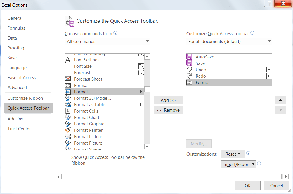
3
Add the «Form» button to Excel. By default, the «Form» button isn’t included in Excel. You can add it to Excel’s list of «Quick Access» icons that appear in the top-left corner of the window by doing the following:
- Click File.
- Click Options in the bottom-left side of the window.
- Click Quick Access Toolbar on the left side of the window.
- Click the «Choose commands from» drop-down box at the top of the window.
- Click All Commands.
- Scroll down until you reach Form, then click it.
- Click Add >> in the middle of the window.
- Click OK.
-
4
Enter your column headers. Type the name of the column into which you want to add data into the top cell in each column you want to use.
- For example, if you’re creating a form that lists different baked items, you might type «Pumpkin Bread» into cell A1, «Muffins» into cell B1, and so on.
-
5
Select your column headers. Click and hold the left-most column header, then drag your mouse right to the right-most column header. You can then release your mouse button.
-
6
Click the «Form» button. It’s the box-shaped icon in the upper-left side of the Excel window, just right of the right-facing «Redo» button.
-
7
Click OK when prompted. Doing so opens the Form pop-up window.
-
8
Enter the data for your first row. Type whatever you want to add into each column header’s text box.
-
9
Click New. It’s in the upper-right side of the pop-up window. Doing this will automatically enter your typed data into the spreadsheet under the appropriate column headers.
-
10
Enter subsequent rows of information. Each time you finish filling out the data entry fields, clicking New will enter your data and start a new row.
-
11
Close the data entry form. Click Close on the right side of the window to do so. Your data should now be completely entered below the appropriate column headers.


Advertisement
-
1
Open Excel. Click or double-click the Excel app icon, which resembles a white «X» on a dark-green background.
-
2
Click Blank workbook. It’s in the upper-left side of the page.
-
3
Enable the Developer tab. The Developer tab is where you’ll find the option to insert form buttons, but it isn’t included in Excel by default. To enable it, do the following:[1]
- Windows — Click File, click Options, click Customize Ribbon, check the «Developer» box, and click OK.
- Mac — Click Excel, click Preferences…, click Authoring under the «View» heading, and click Developer tab. You can then close the window.
-
4
Enter your form’s data. Type in whatever data you want users to be able to select in your form.
- This step will vary depending on the information you want to use in your form.
-
5
Click the Developer tab. It’s at the top of the Excel window.
-
6
Click Insert. This option is in the «Controls» section of the Developer toolbar. Clicking it prompts a drop-down menu to appear.
- Skip this step on a Mac.
-
7
Select a form control. Click the type of control you want to use for your spreadsheet.
- For example, if you want to add a checkbox to your form, you would click the checkbox icon.
-
8
Click anywhere on the spreadsheet. Doing so will place your control button on the spreadsheet.
- You can click and drag your control to the location in which you want to anchor it.
-
9
Right-click the form control icon. A drop-down menu will appear.
- On a Mac, hold down Control while clicking the icon.
-
10
Click Format Control…. It’s at the bottom of the drop-down menu.
-
11
Edit your form control button. Depending on the button you selected, your options will vary; in most cases, you’ll be able to select a cell range or a target cell by clicking the arrow to the right of the «Cell range» or «Target cell» text box and then selecting cells (or a cell) that contain your form’s data.
- For example, if you wanted to create a drop-down menu with a list of numbers, you would click the arrow to the right of the «Cell range» text box and then click and drag your mouse down a column of numbers in your spreadsheet.
-
12
Click OK. It’s at the bottom of the window. Doing so saves your settings and applies them to your spreadsheet.
- At this point, you can proceed with adding other form buttons to your spreadsheet.
-
13
Protect your spreadsheet. Once you’ve finished adding form buttons to your spreadsheet, you can prevent people from moving or removing the buttons by protecting the spreadsheet:
- Windows — Click Review in the Excel toolbar, click Protect Sheet, make sure that any options other than «Select locked cells» and «Select unlocked cells» are unchecked, enter a password to unlock the document, and click OK. You can then re-enter the password when prompted to finish locking the sheet.
- Mac — Click Tools at the top of the screen, select Protection, click Protect Sheet in the pop-out menu, make sure that any options other than «Select locked cells» and «Select unlocked cells» are unchecked, enter a password to unlock the document, and click OK. You can then re-enter the password when prompted to finish locking the sheet.


Advertisement
Ask a Question
200 characters left
Include your email address to get a message when this question is answered.
Submit
Advertisement
Video
Thanks for submitting a tip for review!
About This Article
Article SummaryX
1. Open a blank workbook.
2. Add the «Form» button to Excel.
3. Create column headers.
4. Select the column headers.
5. Click Form.
6. Click OK.
7. Enter the first row data and click New.
8. Enter additional rows.
9. Click Close.
Did this summary help you?
Thanks to all authors for creating a page that has been read 419,834 times.
Is this article up to date?
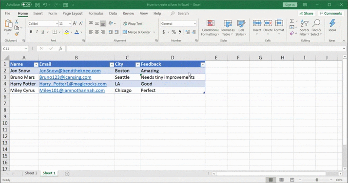
Let’s say you own a hot sauce company.
Having an Excel customer feedback form will tell you how tasty 😋 and spicy 🌶️ your sauce is. Beats asking people individually, any day, right?
So whether you want to survey customers, take client feedback, or collect data from employees, Excel forms can be handy.
But how do you create a form in Excel in the first place?!
In this article, you’ll learn how to create a form in Excel.
We’ll also go over its limitations and suggest an alternative tool to create forms easily.
Make way for the hot sauce feedback with a quick Excel form!
What Are Excel Forms?
An Excel form is a data collection tool from Microsoft Excel. It’s basically a dialog box containing fields for a single record.
In each record, you can enter up to 32 fields, and your Excel worksheet column headers become the form field names.
What are the benefits of using an Excel data entry form?
Now Excel isn’t easy.
Its endless cells make it difficult to know where to feed what data.
Like trying to understand what ‘mild’ means when all you know and love is spicy sauces!
This is why people use Excel forms to make quick data entries in the right fields without scrolling up and down the whole worksheet.
No more entering data into an Excel spreadsheet row after row after row after row…

An Excel data entry form lets you:
- View more data without scrolling up and down
- Include data validation
- Reduce chances of human errors
Sounds quite helpful. So let’s learn how to create an Excel form.
How To Create A Form In Excel?
Before you cook up a form in Excel, you gotta do the prep work.
First, you must have your columns or fields ready.
They’re your raw ingredients, like chili peppers or ginger, ready for your sauce.
You also have to find the ‘Form’ option.
No worries.
We’ll help you make a table, find the ‘Form’ option, and create an Excel form using a step-by-step guide:
Step 1: Make a quick Excel table
Open an Excel spreadsheet, and you’ll start on the first sheet tab (by default).
For this form, you’re the owner of a hot sauce company.
And we’re gonna make a customer feedback form for your delicious sauce.
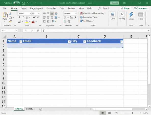
Here’s an example of the columns you can add to your Excel worksheet:
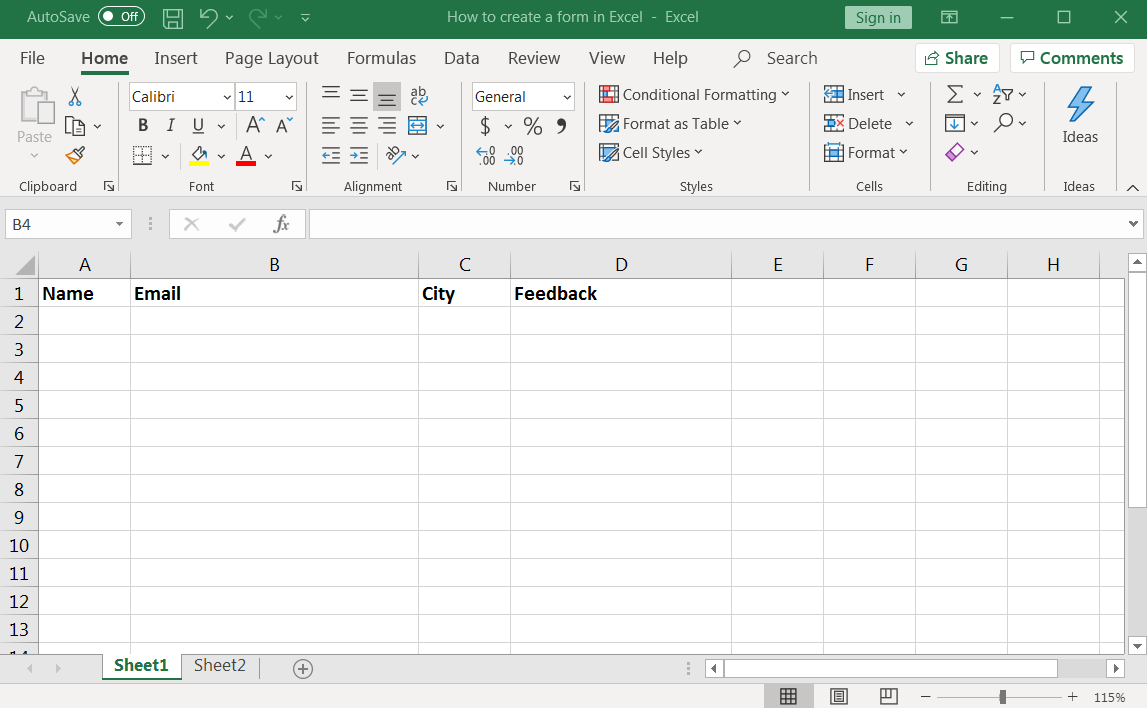
Now you have to convert your column names into a table.
Just select the column headers > click on Insert > Tables > Table.
A tiny dialog box should pop up. Make sure to tick the My table has headers checkbox.

Click on OK, and you should get an Excel table as shown in the image below.
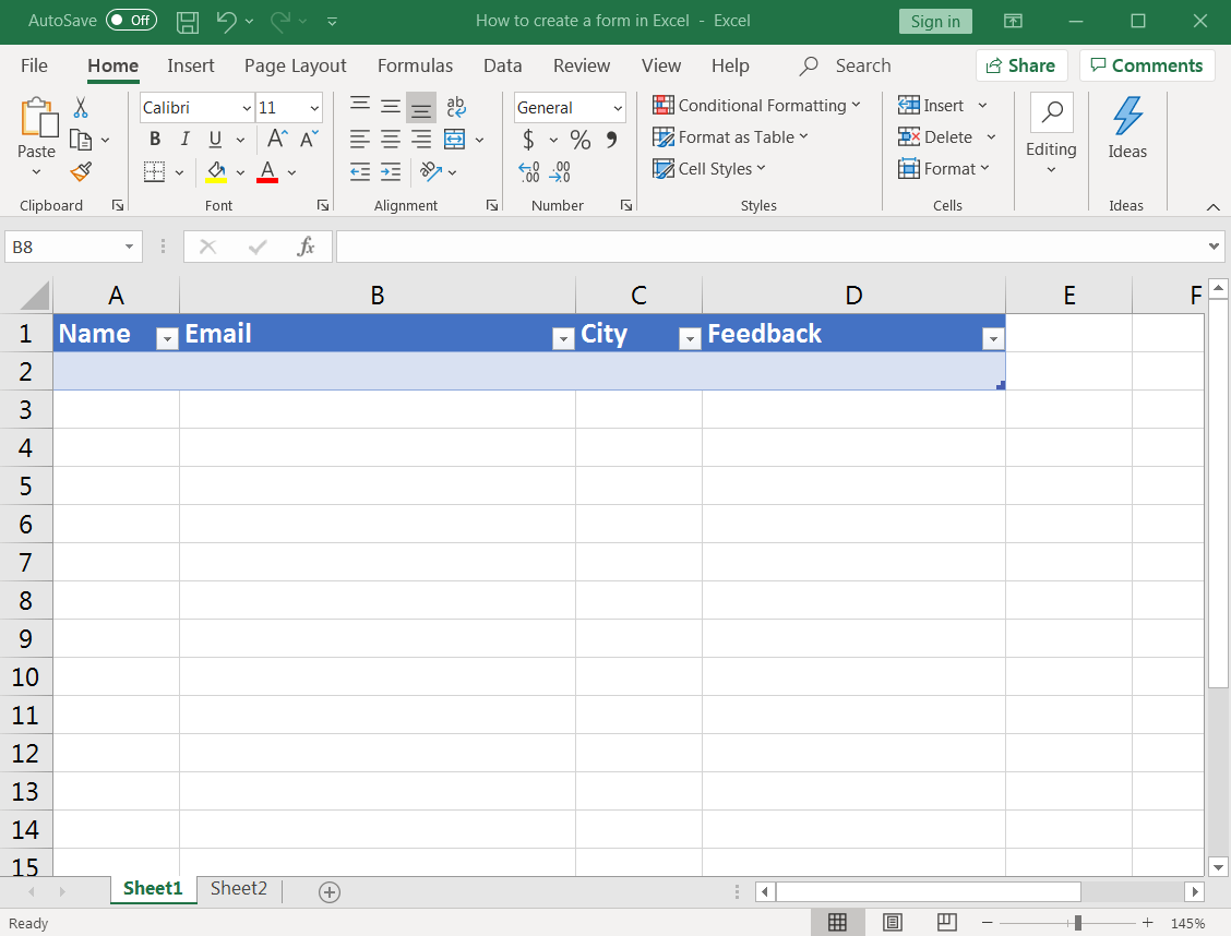
Here, you can adjust the column width depending on the data the field may contain.
Step 2: Add data entry form option to the Excel ribbon
Take a good look at your Excel worksheet.
Check the row of tabs and icons at the top of the Excel window (ribbon). You won’t find the option to use a data entry form in any ribbon tab.

Don’t worry. It’s perfectly normal.
You have to add the ‘form’ option to the Excel sheet ribbon. To do this:
- Right-click on any of the existing icons you see in the ribbon or toolbar
- Click on Customize the Ribbon.
- An Excel Options dialog box should pop up
- Select All Commands from the drop-down list
- Scroll down the list of commands and select Form
- Now click on Add
Did it work? If yes, congratulations!
In case it didn’t allow you to add the Form command button or option, just click on New Tab > Rename > Name it ‘Form’ > click OK.
Then, click on New Group > Add.
Make sure the Form option is selected when you click Add.
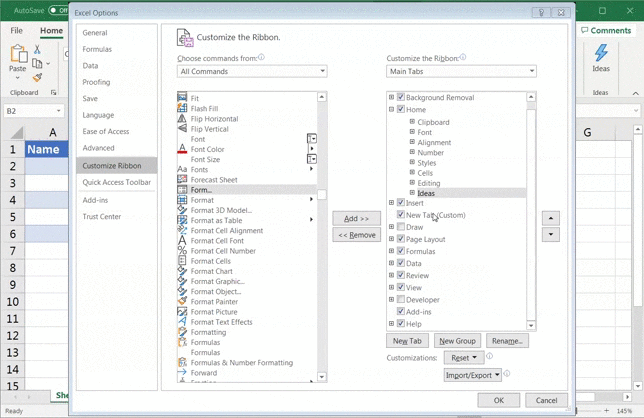
And that’s it! You have finally completed adding the Form icon to the ribbon.
To access it quickly in your workbook, click on Quick Access Toolbar in the same Excel Options dialog box you used earlier.
Select Form under All Commands > click Add. Then, hit enter.
And voila!
You’ll notice the Form button or icon appear on the green area at the top of the Excel workbook in the quick access toolbar.
Bonus: Make a Fillable Form in Word!
Step 3: Enter form data
Now, you can click on any cell in your table and then on the Form icon to input form data.
A dialog box should open with the field names and some button options such as New, Delete, Restore, and criteria button.
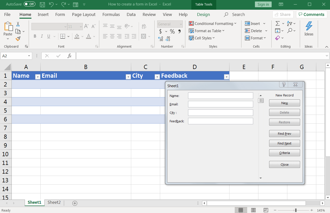
This is a customized data entry form based on the fields in our data.
Enter the desired data in the fields and click on the form button New.
That should make the data appear in your Excel table.
Click on Close to leave the dialog box and view your data table.
Repeat the process till you have entered all the data you want.
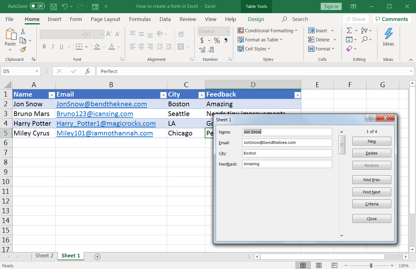
Step 4: Restrict data entry based on conditions
If your hot sauce form contains certain criteria or rules for filling fields, data validation can be useful. It ensures your customers’ data conforms to a few conditions.
For example, you want the sauce feedback field to only accept short texts. So you can create a data validation rule to allow only a specific text length.
If a customer enters feedback longer than what you want, it will not be allowed, and they will see an error.
Here’s how you can set these data entry form control conditions:
- Select the cell or cells where you want to add a data validation rule. In this example, we have selected cells under the feedback column (D2-D5)
- Click the Data tab > Data Validation icon > select Data Validation from the drop-down list
- The Data Validation dialog box will appear. Under Settings, select Text length from the Allow drop-down. Then choose the text length condition under Data and the number of characters. Click OK to apply the rules
Here we chose the condition ‘less than’ and set the feedback character limit to a maximum ‘10’.
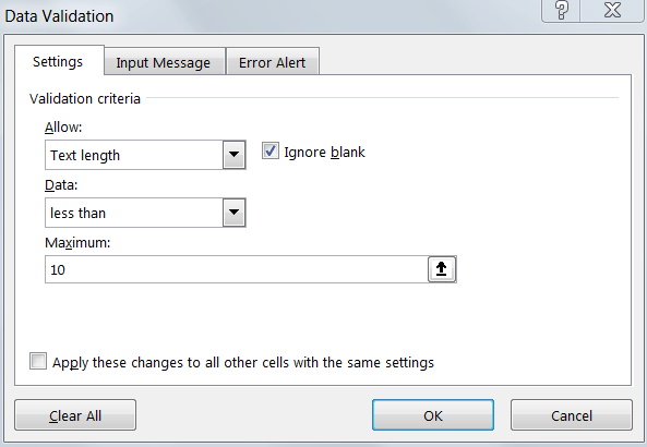
Now, when you use the data entry form to enter text in the feedback column, and if it isn’t a text under ten characters, it won’t be allowed.
You’ll be alerted with a sound and this error message.

But this is just an example.
Don’t stop your customers from singing praises for your sauce! 😛
Data validation only helps ensure people don’t fill in wrong data in the fields.
I mean, what if someone enters the feedback ‘amazing’ in the name field?
Great idea for a name, but no help for your data collection efforts! 😜
Step 5: Start collecting data
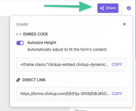
You can now collect data using any of these options:
- Ask customers to fill the form by sharing the Excel file with them. Invite them using their email address or copy and share the spreadsheet link
- Send a copy of the form as an email attachment
- Fill in the data yourself as the customers give you feedback
You’ll find all these options by clicking on share on the top right corner of your sheet.
Note: This process is different from creating a custom form using Excel VBA (Visual Basics for Application). Excel VBA is a Microsoft Excel programming language used to automate tasks and perform other functions such as create a text box, userform, etc.
The Excel VBA user form isn’t an ideal option since it’s even more complicated to set up.
Bonus: Use Jotform to create forms!
3 Limitations Of Creating Forms In Excel
Excel does kind of speed up the data entry process using the form functionality.
However, it doesn’t make it fun, and that’s just one of its limitations.
Here are some more limitations that might make you want to reconsider using an Excel data entry form:
1. Formula restrictions
Excel formulas have split the world into two teams.
One finds it convenient, and the other finds it impossible.
Like how some people love hot sauces while others prefer something sweeter.
But with forms, you straight-up can’t enter an Excel formula into a data form field.
You just can’t.
Then why even use Excel?!
2. Field limit
Clearly, there’s a limit to how many fields there can be in an Excel form.
What do you do when you want more than 32 columns (fields)?
Wouldn’t it be easier to have a tool that wasn’t as complex as MS Excel and didn’t restrict fields?
3. Not the most user-friendly form
Excel can be difficult for many users because of the different functions and rules.
To create form in Excel, you must add a feature to the toolbar.
What’s with the hide and seek, Excel?
Oh, and it’s absolutely not user-friendly for Mac users.
Cause guess what?
The form command doesn’t even exist in the Mac version! *scoff*
Having second thoughts about Excel? Here are the top Excel alternatives
Clearly, you need a tool that can make up for all the Excel form drawbacks and do more.
Good news!
Introducing ClickUp, one of the world’s highest-rated productivity tool used by teams in small and big companies.
Related Resources:
- How to Create a Project Timeline in Excel
- How to Make a Calendar in Excel
- How to Create an Org Chart in Excel
- How to Make a Graph in Excel
- How to Make a KPI Dashboard in Excel
- How to Make an Excel Database
- How to Show Dependencies in Excel
Create Effortless Forms Using ClickUp
ClickUp is the ultimate all-in-one tool to create forms.
What you’re looking for is our Form view.
And unlike Excel, we don’t hide it. Because we’re proud of it! 😎

We also want you to find it without reading a guide like you just did.
Check out these ClickUp Form tips for educators!🍎
To build a form in ClickUp, you must add a form view in three simple steps:
- Open a List, Space, or Folder of your choice
- Click on the + button and select Form
- Name it and add a description
Ensure that the name is something catchy or appropriate depending on the purpose of your form.
How’s ‘Fire cannot kill a dragon’ for a catchy hot sauce form title?
(Warning: Only people who love their spice will get this 😎)
Now let’s build this form!
You’ll find a bunch of fields on the left panel in the form view. Drag and drop them on your form, and that’s how easy it is to add a field.
The panel doesn’t have the field you’re looking for? No worries!
Just click on the field’s title to rename it.

But wait, we’re not close to done being awesome.
Did you know you can also add your company branding in the form view?
After you complete it, it’s time to share your form.
Spot the ‘Share’ icon on the top right of the form view. Click on it to copy the direct link for your form to share it with anyone you like.
Or you can build the form into a page via the HTML code through the ‘embed code’ section.
Bonus: Form building tips for ClickUp.
And lastly, we’re pretty sure you won’t need any other tool if you have ClickUp forms.
But if you prefer other apps like Google Forms, ClickUp can easily integrate with them too. The integration converts Google Forms responses into ClickUp tasks automatically.
What’s more?
ClickUp has so many more awesome features in store for you.
Here’s a sneak peek at some of the many features ClickUp has to offer:
- View tasks in a spreadsheet format with the Table view
- Create tasks and reminders without the internet with offline mode
- Assign a single task to multiple assignees
- Create workflows with custom statuses
- Set reminders, so you don’t miss out on important tasks
- Share all your views with anyone using public sharing
- Integrate with all your favorite tools, including Trello, Microsoft Teams, Google Drive, etc.
- Import an Excel file into ClickUp by saving it as a CSV
- Track task durations using the native time tracker
Excel Or ClickUp: What’s Hot? 🔥
An Excel form is less of a form creator and more of an easy data entry application.
It can help you avoid mistakes if data entry is part of your daily work.
However, when it comes to creating forms, Excel doesn’t seem ideal.
Instead, try ClickUp. It’s a powerful project management tool that lets you create custom forms using a simple drag and drop functionality.
If there’s anything you want to do beyond that, ClickUp has a long list of features, including Mind maps, Workload view, Notepad, priorities, and more.
So you never have to leave the platform for anything. Save your precious time, people!
Use ClickUp for free and create red-hot forms that nobody can resist!🌶️

Create a form with Microsoft Forms
- Sign in to Office 365 with your school or work credentials.
- Open the Excel workbook in which you want to insert a form.
- Click Insert > Forms > New Form to begin creating your form.
- A new tab, Microsoft Forms, will open.
- A default title for your form will be provided.
Contents
- 1 How do you create a form in Excel?
- 2 How do you make Excel look like a fillable form?
- 3 Can you create a Microsoft form from Excel?
- 4 How do I create a form?
- 5 How do I create a fillable form?
- 6 How do I create a form in Excel 2016?
- 7 What is form in Excel?
- 8 How do I create a SharePoint form in Excel?
- 9 Where is forms in Excel?
- 10 Which object is used to create a form?
- 11 What are examples of forms?
- 12 How do I create a SharePoint form?
- 13 What is the best software to create fillable forms?
- 14 What is the best program to create forms?
- 15 How do I create a form field in Word?
- 16 What is Forms for Excel in SharePoint?
- 17 How do you create a fillable table in Microsoft forms?
- 18 How do I link Microsoft Excel to form?
How do you create a form in Excel?
Data Entry Form in Excel
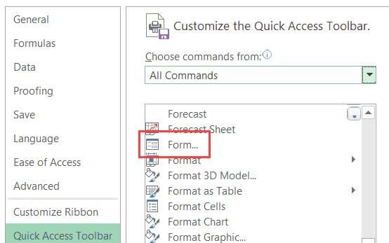
- Right-click on any of the existing icons in the Quick Access Toolbar.
- Click on ‘Customize Quick Access Toolbar’.
- In the ‘Excel Options’ dialog box that opens, select the ‘All Commands’ option from the drop-down.
- Scroll down the list of commands and select ‘Form’.
- Click on the ‘Add’ button.
How do you make Excel look like a fillable form?
1. Create Form in Excel
- STEP 1: Convert your Column names into a Table, go to Insert> Table.
- STEP 2:Let us add the Form Creation functionality to understand how to make a fillable form in Excel.
- STEP 3:Go to Customize Ribbon.
- STEP 4:Under the New Tab, select New Group, and click Add.
Can you create a Microsoft form from Excel?
If you’re working with Excel Online, you can also create forms. Go to the Insert tab ➜ click on the Forms button ➜ select New Form from the menu. This will create a form that’s linked to the current workbook.
How do I create a form?
To create a form in Word that others can fill out, start with a template or document and add content controls.
Start with a form template
- Go to File > New.
- In Search online templates, type Forms or the type of form you want and press ENTER.
- Choose a form template, and then select Create or Download.
How do I create a fillable form?
How to create fillable PDF files:
- Open Acrobat: Click on the “Tools” tab and select “Prepare Form.”
- Select a file or scan a document: Acrobat will automatically analyze your document and add form fields.
- Add new form fields: Use the top toolbar and adjust the layout using tools in the right pane.
- Save your fillable PDF:
How do I create a form in Excel 2016?
How Do I Create a Data Entry Form in Excel 2016?
- On the chosen sheet, highlight the number of columns needed.
- Open the Tables tab, click New, click Insert Table with Headers.
- Change the default column headers, and adjust the width of columns if necessary.
- Open the Data menu and click Form…
- The form will appear.
What is form in Excel?
A form contains controls, such as boxes or dropdown lists, that can make it easier for people who use your worksheet to enter or edit data. To find out more about templates you can download, see Excel templates.
How do I create a SharePoint form in Excel?
To use Forms for Excel head to OneDrive, SharePoint and Teams. Navigate to the location where you want to store your form results > click on New > select Forms for Excel. You will then be asked to name the workbook associated with your form.
Where is forms in Excel?
Add the Form button to the ribbon
- Click the arrow next to the Quick Access Toolbar, and then click More Commands.
- In the Choose commands from box, click All Commands, and then select the Form button in the list.
- Click Add, and then click OK.
Which object is used to create a form?
Discussion Forum
| Que. | Which object is used to create a form? |
|---|---|
| b. | Tables only |
| c. | Tables and reports |
| d. | Queries and reports |
| Answer:Tables and Queries |
What are examples of forms?
The definition of form is the shape of a person, animal or thing or a piece of paperwork that needs to be filled out. An example of form is the circular shape of an apple. An example of form is a job application. Form is defined as to make or construct something.
How do I create a SharePoint form?
New form
- Click Add new form.
- In the panel on the right, provide a name for your new form.
- Click Create.
- Microsoft Forms will open in a new tab. See below for steps to create a new form.
- When you’re done creating your form, go back to your SharePoint in Microsoft 365 page.
What is the best software to create fillable forms?
Adobe Acrobat Pro DC is the best app to create fillable forms, and consists of three main functions, Acrobat DC, Adobe Document Cloud, and Acrobat Reader. The first one enables you to edit PDFs, the second one keeps PDFs in sync in its cloud storage, and the last one is to read, print, and sign PDFs.
What is the best program to create forms?
Best online form builders of 2021
- Hubspot Free Online Form Builder.
- Gravity Forms.
- Typeform.
- Wufoo.
- Microsoft Forms.
- Formstack.
- Paperform.
- Formsite.
How do I create a form field in Word?
Click in your Word document wherever you wish to insert a Form Field. On the Legacy Forms menu click the first icon to insert a Form Field. Right-click on the Form Field and select Properties. Then provide a name for the field in the Bookmark section.
What is Forms for Excel in SharePoint?
Forms for Excel includes new features such as response time, responder name, images, videos, themes, and branching logic. Use any of the following entry points: OneDrive for Business: Click + New. Document library of modern SharePoint team sites (O365 group backed): Click + New.
How do you create a fillable table in Microsoft forms?
On the form template, place the cursor where you want to insert the layout table. On the Tables toolbar, click Insert, and then click Layout Table. In the Insert Table dialog box, enter the number of columns and rows that you want to include in the table.
How do I link Microsoft Excel to form?
Sign in to Office 365 with your school or work credentials. Open the Excel workbook in which you want to insert a form. Click Insert > Forms > New Form to begin creating your form. Note: To enable the Forms button, make sure your Excel workbook is stored in OneDrive for Business.
Содержание
- Применение инструментов заполнения
- Способ 1: встроенный объект для ввода данных Excel
- Способ 2: создание пользовательской формы
- Вопросы и ответы

Для облегчения ввода данных в таблицу в Excel можно воспользоваться специальными формами, которые помогут ускорить процесс заполнения табличного диапазона информацией. В Экселе имеется встроенный инструмент позволяющий производить заполнение подобным методом. Также пользователь может создать собственный вариант формы, которая будет максимально адаптирована под его потребности, применив для этого макрос. Давайте рассмотрим различные варианты использования этих полезных инструментов заполнения в Excel.
Применение инструментов заполнения
Форма заполнения представляет собой объект с полями, наименования которых соответствуют названиям колонок столбцов заполняемой таблицы. В эти поля нужно вводить данные и они тут же будут добавляться новой строкой в табличный диапазон. Форма может выступать как в виде отдельного встроенного инструмента Excel, так и располагаться непосредственно на листе в виде его диапазона, если она создана самим пользователем.
Теперь давайте рассмотрим, как пользоваться этими двумя видами инструментов.
Способ 1: встроенный объект для ввода данных Excel
Прежде всего, давайте узнаем, как применять встроенную форму для ввода данных Excel.
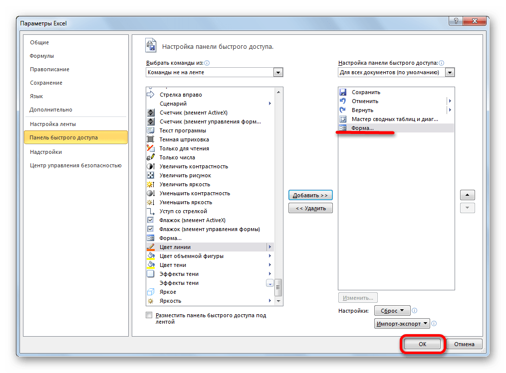
- Нужно отметить, что по умолчанию значок, который её запускает, скрыт и его нужно активировать. Для этого переходим во вкладку «Файл», а затем щелкаем по пункту «Параметры».
- В открывшемся окне параметров Эксель перемещаемся в раздел «Панель быстрого доступа». Большую часть окна занимает обширная область настроек. В левой её части находятся инструменты, которые могут быть добавлены на панель быстрого доступа, а в правой – уже присутствующие.
В поле «Выбрать команды из» устанавливаем значение «Команды не на ленте». Далее из списка команд, расположенного в алфавитном порядке, находим и выделяем позицию «Форма…». Затем жмем на кнопку «Добавить».
- После этого нужный нам инструмент отобразится в правой части окна. Жмем на кнопку «OK».
- Теперь данный инструмент располагается в окне Excel на панели быстрого доступа, и мы им можем воспользоваться. Он будет присутствовать при открытии любой книги данным экземпляром Excel.
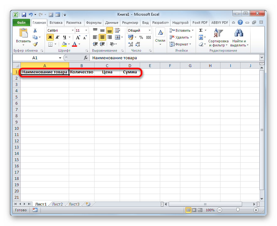
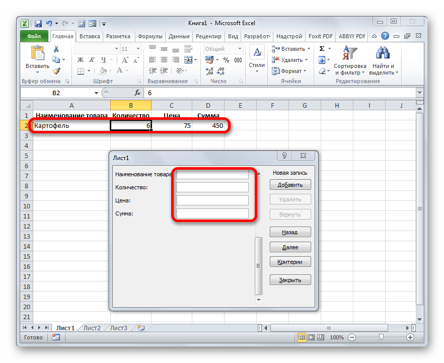
- Теперь, чтобы инструмент понял, что именно ему нужно заполнять, следует оформить шапку таблицы и записать любое значение в ней. Пусть табличный массив у нас будет состоять из четырех столбцов, которые имеют названия «Наименование товара», «Количество», «Цена» и «Сумма». Вводим данные названия в произвольный горизонтальный диапазон листа.
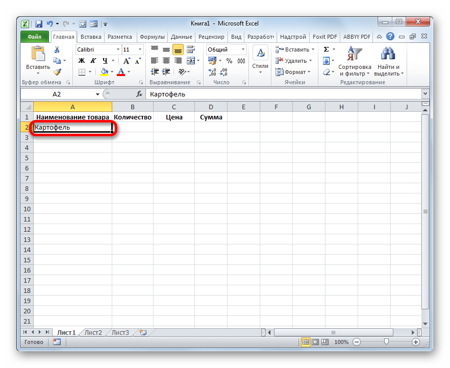
- Также, чтобы программа поняла, с каким именно диапазонам ей нужно будет работать, следует ввести любое значение в первую строку табличного массива.
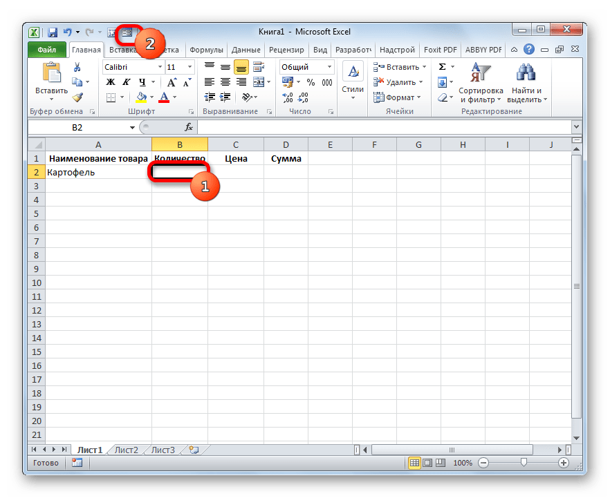
- После этого выделяем любую ячейку заготовки таблицы и щелкаем на панели быстрого доступа по значку «Форма…», который мы ранее активировали.
- Итак, открывается окно указанного инструмента. Как видим, данный объект имеет поля, которые соответствуют названиям столбцов нашего табличного массива. При этом первое поле уже заполнено значением, так как мы его ввели вручную на листе.
- Вводим значения, которые считаем нужными и в остальные поля, после чего жмем на кнопку «Добавить».
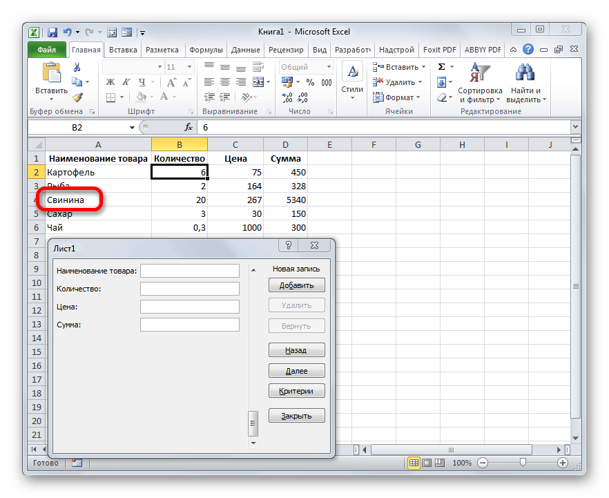
- После этого, как видим, в первую строку таблицы были автоматически перенесены введенные значения, а в форме произошел переход к следующему блоку полей, который соответствуют второй строке табличного массива.
- Заполняем окно инструмента теми значениями, которые хотим видеть во второй строке табличной области, и снова щелкаем по кнопке «Добавить».
- Как видим, значения второй строчки тоже были добавлены, причем нам даже не пришлось переставлять курсор в самой таблице.
- Таким образом, заполняем табличный массив всеми значениями, которые хотим в неё ввести.
- Кроме того, при желании, можно производить навигацию по ранее введенным значениям с помощью кнопок «Назад» и «Далее» или вертикальной полосы прокрутки.
- При необходимости можно откорректировать любое значение в табличном массиве, изменив его в форме. Чтобы изменения отобразились на листе, после внесения их в соответствующий блок инструмента, жмем на кнопку «Добавить».
- Как видим, изменение сразу произошло и в табличной области.
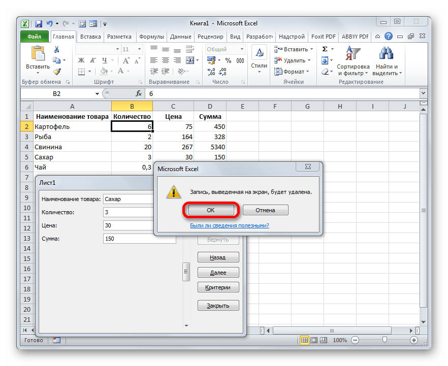
- Если нам нужно удалить, какую-то строчку, то через кнопки навигации или полосу прокрутки переходим к соответствующему ей блоку полей в форме. После этого щелкаем по кнопке «Удалить» в окошке инструмента.
- Открывается диалоговое окно предупреждения, в котором сообщается, что строка будет удалена. Если вы уверены в своих действиях, то жмите на кнопку «OK».
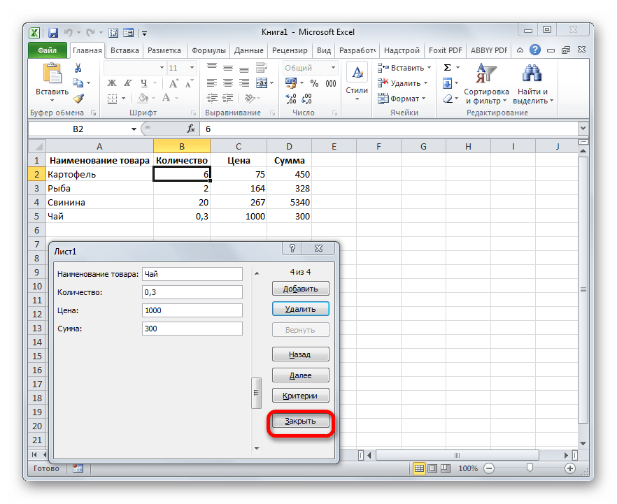
- Как видим, строчка была извлечена из табличного диапазона. После того, как заполнение и редактирование закончено, можно выходить из окна инструмента, нажав на кнопку «Закрыть».
- После этого для предания табличному массиву более наглядного визуального вида можно произвести форматирование.


Способ 2: создание пользовательской формы
Кроме того, с помощью макроса и ряда других инструментов существует возможность создать собственную пользовательскую форму для заполнения табличной области. Она будет создаваться прямо на листе, и представлять собой её диапазон. С помощью данного инструмента пользователь сам сможет реализовать те возможности, которые считает нужными. По функционалу он практически ни в чем не будет уступать встроенному аналогу Excel, а кое в чем, возможно, превосходить его. Единственный недостаток состоит в том, что для каждого табличного массива придется составлять отдельную форму, а не применять один и тот же шаблон, как это возможно при использовании стандартного варианта.
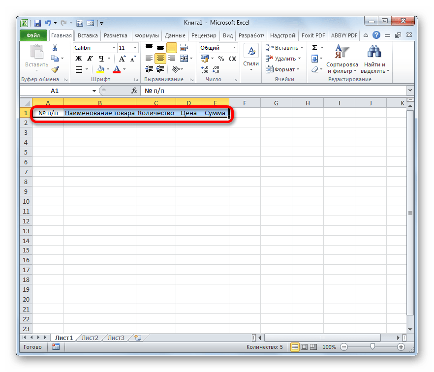
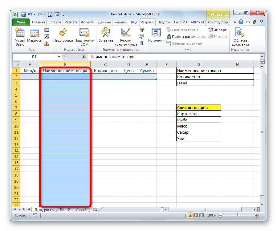
- Как и в предыдущем способе, прежде всего, нужно составить шапку будущей таблицы на листе. Она будет состоять из пяти ячеек с именами: «№ п/п», «Наименование товара», «Количество», «Цена», «Сумма».
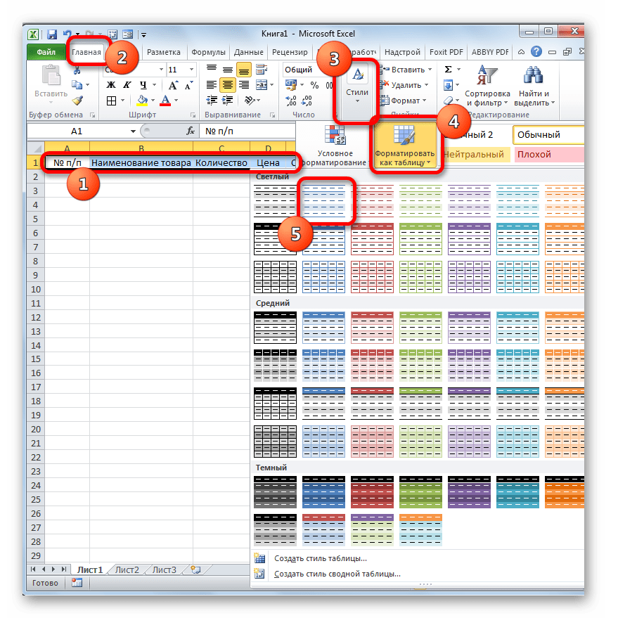
- Далее нужно из нашего табличного массива сделать так называемую «умную» таблицу, с возможностью автоматического добавления строчек при заполнении соседних диапазонов или ячеек данными. Для этого выделяем шапку и, находясь во вкладке «Главная», жмем на кнопку «Форматировать как таблицу» в блоке инструментов «Стили». После этого открывается список доступных вариантов стилей. На функционал выбор одного из них никак не повлияет, поэтому выбираем просто тот вариант, который считаем более подходящим.
- Затем открывается небольшое окошко форматирования таблицы. В нем указан диапазон, который мы ранее выделили, то есть, диапазон шапки. Как правило, в данном поле заполнено все верно. Но нам следует установить галочку около параметра «Таблица с заголовками». После этого жмем на кнопку «OK».
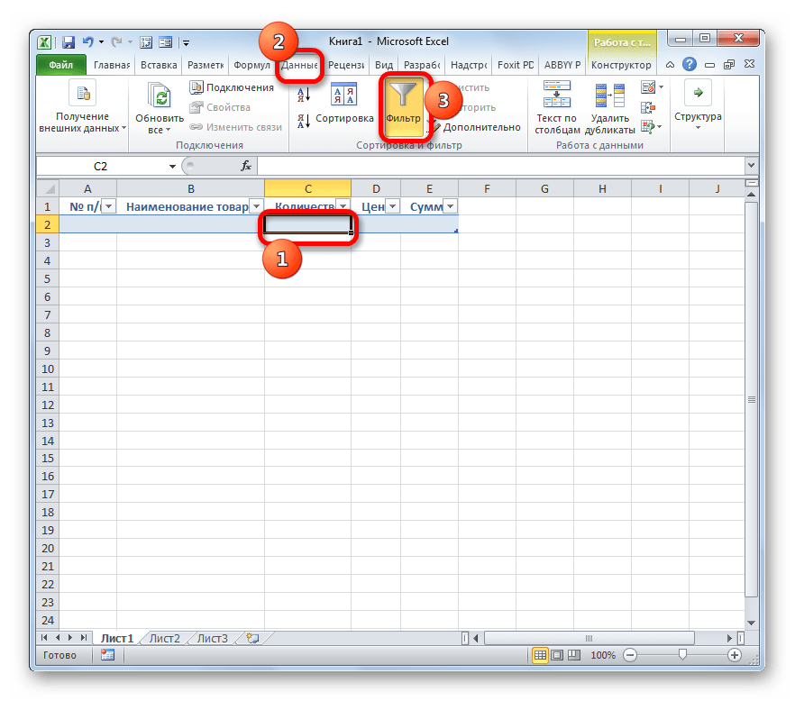
- Итак, наш диапазон отформатирован, как «умная» таблица, свидетельством чему является даже изменение визуального отображения. Как видим, помимо прочего, около каждого названия заголовка столбцов появились значки фильтрации. Их следует отключить. Для этого выделяем любую ячейку «умной» таблицы и переходим во вкладку «Данные». Там на ленте в блоке инструментов «Сортировка и фильтр» щелкаем по значку «Фильтр».

Существует ещё один вариант отключения фильтра. При этом не нужно даже будет переходить на другую вкладку, оставаясь во вкладке «Главная». После выделения ячейки табличной области на ленте в блоке настроек «Редактирование» щелкаем по значку «Сортировка и фильтр». В появившемся списке выбираем позицию «Фильтр».
- Как видим, после этого действия значки фильтрации исчезли из шапки таблицы, как это и требовалось.
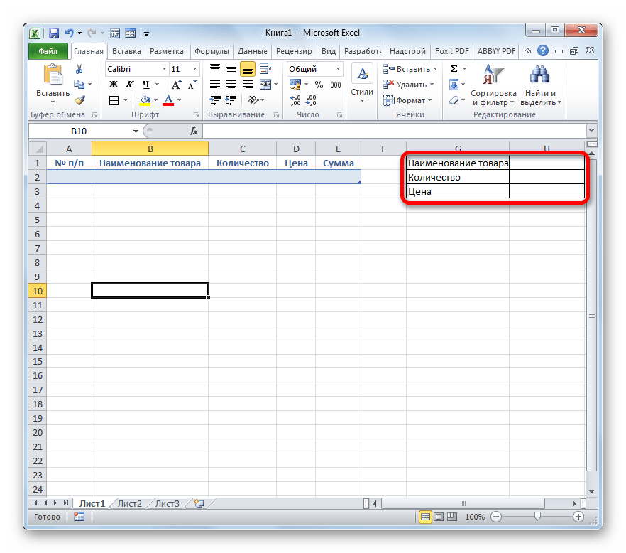
- Затем нам следует создать саму форму ввода данных. Она тоже будет представлять собой своего рода табличный массив, состоящий из двух столбцов. Наименования строк данного объекта будут соответствовать именам столбцов основной таблицы. Исключение составляют столбцы «№ п/п» и «Сумма». Они будут отсутствовать. Нумерация первого из них будет происходить при помощи макроса, а расчет значений во втором будет производиться путем применения формулы умножения количества на цену.
Второй столбец объекта ввода данных оставим пока что пустым. Непосредственно в него позже будут вводиться значения для заполнения строк основного табличного диапазона.
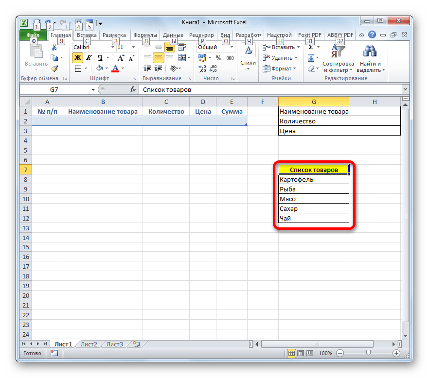
- После этого создаем ещё одну небольшую таблицу. Она будет состоять из одного столбца и в ней разместится список товаров, которые мы будем выводить во вторую колонку основной таблицы. Для наглядности ячейку с заголовком данного перечня («Список товаров») можно залить цветом.
- Затем выделяем первую пустую ячейку объекта ввода значений. Переходим во вкладку «Данные». Щелкаем по значку «Проверка данных», который размещен на ленте в блоке инструментов «Работа с данными».
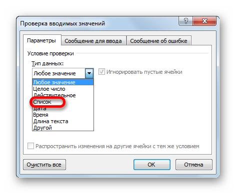
- Запускается окно проверки вводимых данных. Кликаем по полю «Тип данных», в котором по умолчанию установлен параметр «Любое значение».
- Из раскрывшихся вариантов выбираем позицию «Список».
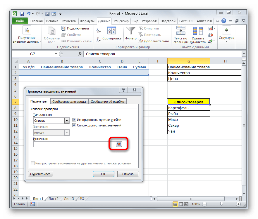
- Как видим, после этого окно проверки вводимых значений несколько изменило свою конфигурацию. Появилось дополнительное поле «Источник». Щелкаем по пиктограмме справа от него левой клавишей мыши.
- Затем окно проверки вводимых значений сворачивается. Выделяем курсором с зажатой левой клавишей мыши перечень данных, которые размещены на листе в дополнительной табличной области «Список товаров». После этого опять жмем на пиктограмму справа от поля, в котором появился адрес выделенного диапазона.
- Происходит возврат к окошку проверки вводимых значений. Как видим, координаты выделенного диапазона в нем уже отображены в поле «Источник». Кликаем по кнопке «OK» внизу окна.
- Теперь справа от выделенной пустой ячейки объекта ввода данных появилась пиктограмма в виде треугольника. При клике на неё открывается выпадающий список, состоящий из названий, которые подтягиваются из табличного массива «Список товаров». Произвольные данные в указанную ячейку теперь внести невозможно, а только можно выбрать из представленного списка нужную позицию. Выбираем пункт в выпадающем списке.
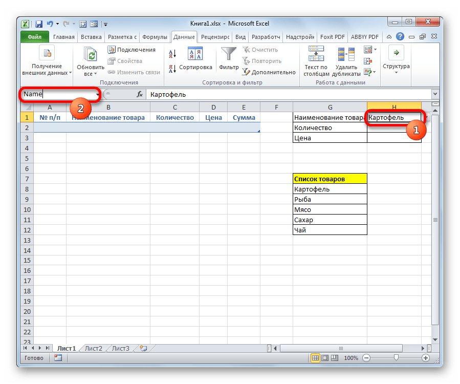
- Как видим, выбранная позиция тут же отобразилась в поле «Наименование товара».
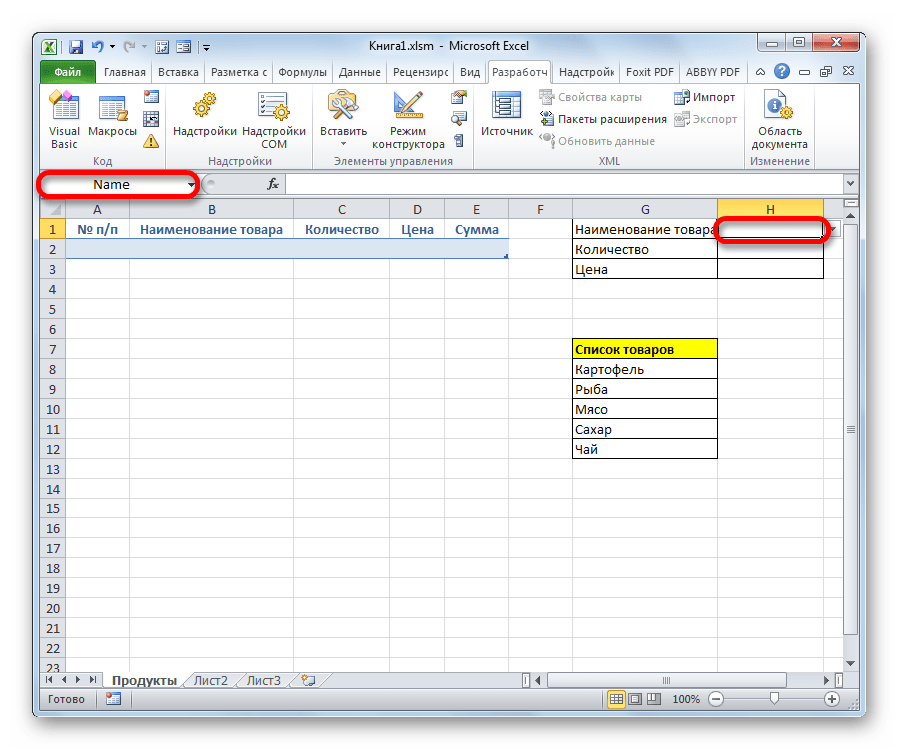
- Далее нам нужно будет присвоить имена тем трем ячейкам формы ввода, куда мы будем вводить данные. Выделяем первую ячейку, где уже установлено в нашем случае наименование «Картофель». Далее переходим в поле наименования диапазонов. Оно расположено в левой части окна Excel на том же уровне, что и строка формул. Вводим туда произвольное название. Это может быть любое наименование на латинице, в котором нет пробелов, но лучше все-таки использовать названия близкие к решаемым данным элементом задачам. Поэтому первую ячейку, в которой содержится название товара, назовем «Name». Пишем данное наименование в поле и жмем на клавишу Enter на клавиатуре.
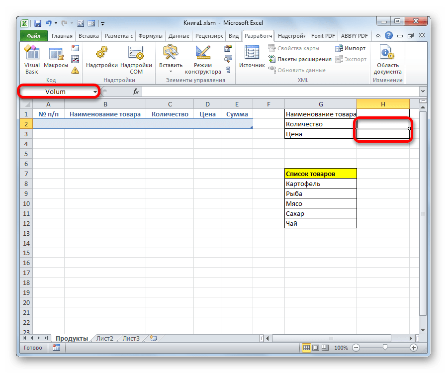
- Точно таким же образом присваиваем ячейке, в которую будем вводить количество товара, имя «Volum».
- А ячейке с ценой – «Price».
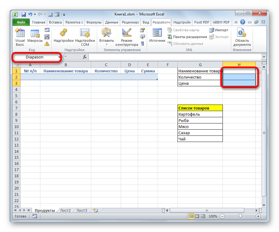
- После этого точно таким же образом даем название всему диапазону из вышеуказанных трех ячеек. Прежде всего, выделим, а потом дадим ему наименование в специальном поле. Пусть это будет имя «Diapason».
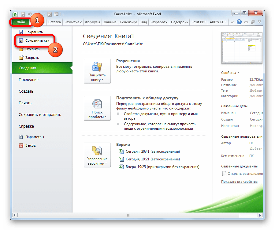
- После последнего действия обязательно сохраняем документ, чтобы названия, которые мы присвоили, смог воспринимать макрос, созданный нами в дальнейшем. Для сохранения переходим во вкладку «Файл» и кликаем по пункту «Сохранить как…».
- В открывшемся окне сохранения в поле «Тип файлов» выбираем значение «Книга Excel с поддержкой макросов (.xlsm)». Далее жмем на кнопку «Сохранить».
- Затем вам следует активировать работу макросов в своей версии Excel и включить вкладку «Разработчик», если вы это до сих пор не сделали. Дело в том, что обе эти функции по умолчанию в программе отключены, и их активацию нужно выполнять принудительно в окне параметров Excel.
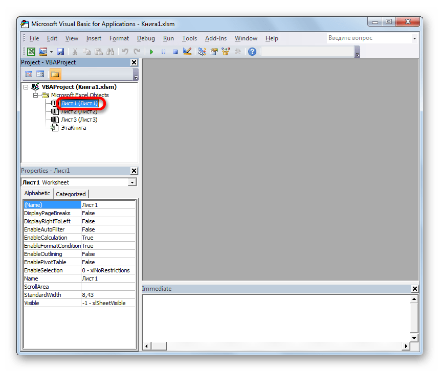
- После того, как вы сделали это, переходим во вкладку «Разработчик». Кликаем по большому значку «Visual Basic», который расположен на ленте в блоке инструментов «Код».
- Последнее действие приводит к тому, что запускается редактор макросов VBA. В области «Project», которая расположена в верхней левой части окна, выделяем имя того листа, где располагаются наши таблицы. В данном случае это «Лист 1».
- После этого переходим к левой нижней области окна под названием «Properties». Тут расположены настройки выделенного листа. В поле «(Name)» следует заменить кириллическое наименование («Лист1») на название, написанное на латинице. Название можно дать любое, которое вам будет удобнее, главное, чтобы в нем были исключительно символы латиницы или цифры и отсутствовали другие знаки или пробелы. Именно с этим именем будет работать макрос. Пусть в нашем случае данным названием будет «Producty», хотя вы можете выбрать и любое другое, соответствующее условиям, которые были описаны выше.
В поле «Name» тоже можно заменить название на более удобное. Но это не обязательно. При этом допускается использование пробелов, кириллицы и любых других знаков. В отличие от предыдущего параметра, который задает наименование листа для программы, данный параметр присваивает название листу, видимое пользователю на панели ярлыков.
Как видим, после этого автоматически изменится и наименование Листа 1 в области «Project», на то, которое мы только что задали в настройках.
- Затем переходим в центральную область окна. Именно тут нам нужно будет записать сам код макроса. Если поле редактора кода белого цвета в указанной области не отображается, как в нашем случае, то жмем на функциональную клавишу F7 и оно появится.
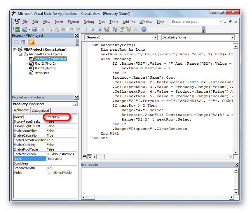
- Теперь для конкретно нашего примера нужно записать в поле следующий код:
Sub DataEntryForm()

Dim nextRow As Long

nextRow = Producty.Cells(Producty.Rows.Count, 2).End(xlUp).Offset(1, 0).Row

With Producty

If .Range("A2").Value = "" And .Range("B2").Value = "" Then

nextRow = nextRow - 1

End If

Producty.Range("Name").Copy

.Cells(nextRow, 2).PasteSpecial Paste:=xlPasteValues

.Cells(nextRow, 3).Value = Producty.Range("Volum").Value

.Cells(nextRow, 4).Value = Producty.Range("Price").Value

.Cells(nextRow, 5).Value = Producty.Range("Volum").Value * Producty.Range("Price").Value

.Range("A2").Formula = "=IF(ISBLANK(B2), """", COUNTA($B$2:B2))"

If nextRow > 2 Then

Range("A2").Select

Selection.AutoFill Destination:=Range("A2:A" & nextRow)

Range("A2:A" & nextRow).Select

End If

.Range("Diapason").ClearContents

End With

End Sub
Но этот код не универсальный, то есть, он в неизменном виде подходит только для нашего случая. Если вы хотите его приспособить под свои потребности, то его следует соответственно модифицировать. Чтобы вы смогли сделать это самостоятельно, давайте разберем, из чего данный код состоит, что в нем следует заменить, а что менять не нужно.
Итак, первая строка:
Sub DataEntryForm()«DataEntryForm» — это название самого макроса. Вы можете оставить его как есть, а можете заменить на любое другое, которое соответствует общим правилам создания наименований макросов (отсутствие пробелов, использование только букв латинского алфавита и т.д.). Изменение наименования ни на что не повлияет.
Везде, где встречается в коде слово «Producty» вы должны его заменить на то наименование, которое ранее присвоили для своего листа в поле «(Name)» области «Properties» редактора макросов. Естественно, это нужно делать только в том случае, если вы назвали лист по-другому.

Теперь рассмотрим такую строку:
nextRow = Producty.Cells(Producty.Rows.Count, 2).End(xlUp).Offset(1, 0).RowЦифра «2» в данной строчке означает второй столбец листа. Именно в этом столбце находится колонка «Наименование товара». По ней мы будем считать количество рядов. Поэтому, если в вашем случае аналогичный столбец имеет другой порядок по счету, то нужно ввести соответствующее число. Значение «End(xlUp).Offset(1, 0).Row» в любом случае оставляем без изменений.

Далее рассмотрим строку
If .Range("A2").Value = "" And .Range("B2").Value = "" Then«A2» — это координаты первой ячейки, в которой будет выводиться нумерация строк. «B2» — это координаты первой ячейки, по которой будет производиться вывод данных («Наименование товара»). Если они у вас отличаются, то введите вместо этих координат свои данные.
Переходим к строке
Producty.Range("Name").CopyВ ней параметр «Name» означат имя, которое мы присвоили полю «Наименование товара» в форме ввода.
В строках
.Cells(nextRow, 2).PasteSpecial Paste:=xlPasteValues

.Cells(nextRow, 3).Value = Producty.Range("Volum").Value

.Cells(nextRow, 4).Value = Producty.Range("Price").Value

.Cells(nextRow, 5).Value = Producty.Range("Volum").Value * Producty.Range("Price").Value
наименования «Volum» и «Price» означают названия, которые мы присвоили полям «Количество» и «Цена» в той же форме ввода.
В этих же строках, которые мы указали выше, цифры «2», «3», «4», «5» означают номера столбцов на листе Excel, соответствующих колонкам «Наименование товара», «Количество», «Цена» и «Сумма». Поэтому, если в вашем случае таблица сдвинута, то нужно указать соответствующие номера столбцов. Если столбцов больше, то по аналогии нужно добавить её строки в код, если меньше – то убрать лишние.
В строке производится умножение количества товара на его цену:
.Cells(nextRow, 5).Value = Producty.Range("Volum").Value * Producty.Range("Price").ValueРезультат, как видим из синтаксиса записи, будет выводиться в пятый столбец листа Excel.
В этом выражении выполняется автоматическая нумерация строк:
If nextRow > 2 Then

Range("A2").Select

Selection.AutoFill Destination:=Range("A2:A" & nextRow)

Range("A2:A" & nextRow).Select

End If
Все значения «A2» означают адрес первой ячейки, где будет производиться нумерация, а координаты «A» — адрес всего столбца с нумерацией. Проверьте, где именно будет выводиться нумерация в вашей таблице и измените данные координаты в коде, если это необходимо.
В строке производится очистка диапазона формы ввода данных после того, как информация из неё была перенесена в таблицу:
.Range("Diapason").ClearContentsНе трудно догадаться, что («Diapason») означает наименование того диапазона, который мы ранее присвоили полям для ввода данных. Если вы дали им другое наименование, то в этой строке должно быть вставлено именно оно.
Дальнейшая часть кода универсальна и во всех случаях будет вноситься без изменений.
После того, как вы записали код макроса в окно редактора, следует нажать на значок сохранения в виде дискеты в левой части окна. Затем можно его закрывать, щелкнув по стандартной кнопке закрытия окон в правом верхнем углу.
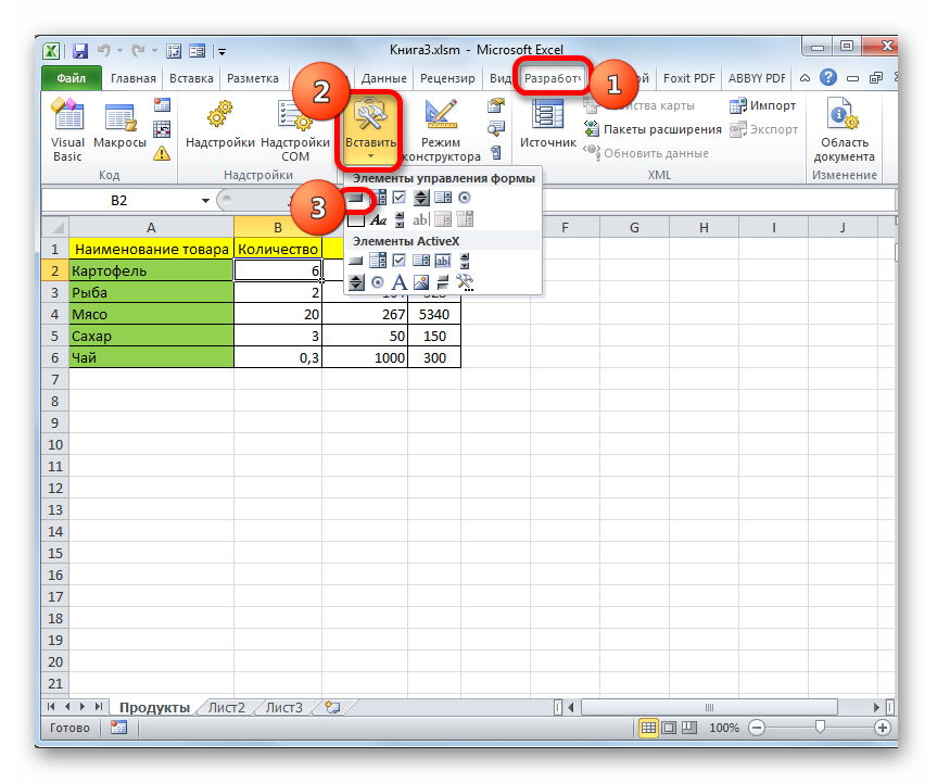
- После этого возвращаемся на лист Excel. Теперь нам следует разместить кнопку, которая будет активировать созданный макрос. Для этого переходим во вкладку «Разработчик». В блоке настроек «Элементы управления» на ленте кликаем по кнопке «Вставить». Открывается перечень инструментов. В группе инструментов «Элементы управления формы» выбираем самый первый – «Кнопка».
- Затем с зажатой левой клавишей мыши обводим курсором область, где хотим разместить кнопку запуска макроса, который будет производить перенос данных из формы в таблицу.
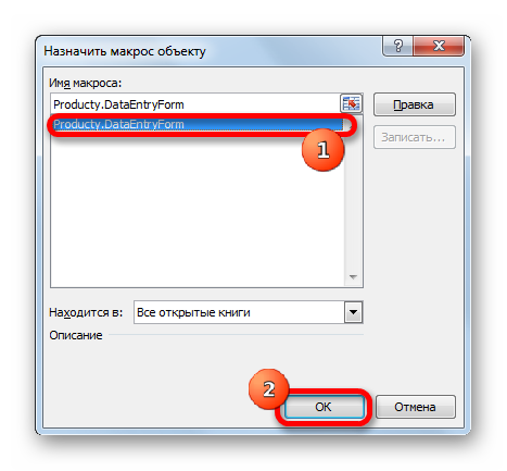
- После того, как область обведена, отпускаем клавишу мыши. Затем автоматически запускается окно назначения макроса объекту. Если в вашей книге применяется несколько макросов, то выбираем из списка название того, который мы выше создавали. У нас он называется «DataEntryForm». Но в данном случае макрос один, поэтому просто выбираем его и жмем на кнопку «OK» внизу окна.
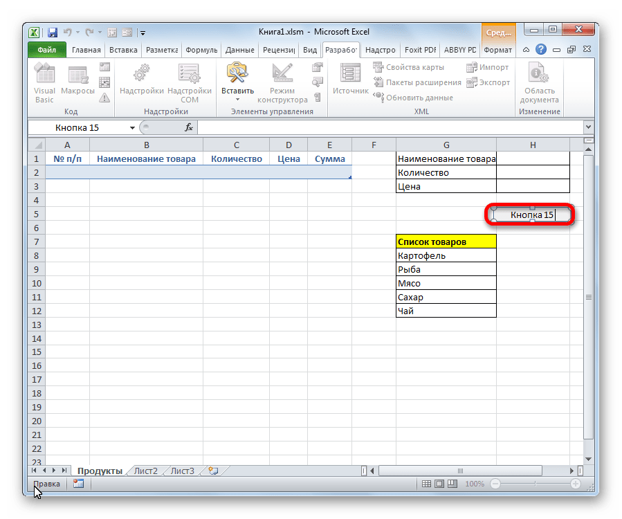
- После этого можно переименовать кнопку, как вы захотите, просто выделив её текущее название.
В нашем случае, например, логично будет дать ей имя «Добавить». Переименовываем и кликаем мышкой по любой свободной ячейке листа.
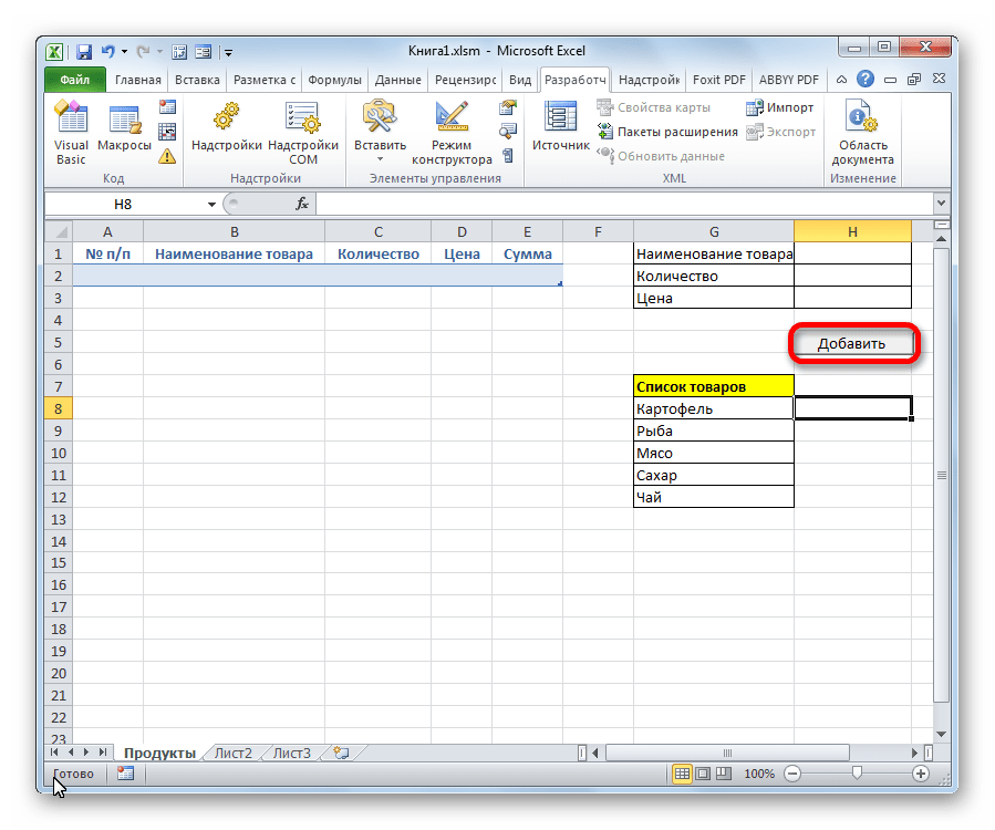
- Итак, наша форма полностью готова. Проверим, как она работает. Вводим в её поля необходимые значения и жмем на кнопку «Добавить».
- Как видим, значения перемещены в таблицу, строке автоматически присвоен номер, сумма посчитана, поля формы очищены.
- Повторно заполняем форму и жмем на кнопку «Добавить».
- Как видим, и вторая строка также добавлена в табличный массив. Это означает, что инструмент работает.


Читайте также:
Как создать макрос в Excel
Как создать кнопку в Excel
В Экселе существует два способа применения формы заполнения данными: встроенная и пользовательская. Применение встроенного варианта требует минимум усилий от пользователя. Его всегда можно запустить, добавив соответствующий значок на панель быстрого доступа. Пользовательскую форму нужно создавать самому, но если вы хорошо разбираетесь в коде VBA, то сможете сделать этот инструмент максимально гибким и подходящим под ваши нужды.
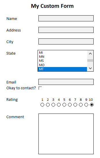
In a previous post, I covered how to add checkboxes. Now, I’m going to go a step further and show you how you can create a form in Excel from start to finish. And at the bottom of the page, you can download a file that you can use for your own custom forms. It will incorporate, list boxes, checkboxes, validation rules, and allow you to move the data onto a separate sheet. For now, let’s start from scratch.
Step 1: Determine the data you want and how it should be entered
The first step in creating a form in Excel is determining what information you want to collect. In this example, I’m just going to include name, address, city, state, email, a checkbox to confirm if it is okay to contact the person, a rating, and an area for comments. It is also important to determine how users should enter these values. While it’s easy to leave everything as text, that can make it difficult to ensure someone doesn’t enter invalid data. And if the data is not useful, it will defeat the purpose of the form.
Here are the types of inputs I’m going to use for my fields:
- Name: Text
- Address: Text
- City: Text
- State: List box
- Email: Text
- Contact confirmation: Checkbox
- Rating: Radio button
- Comments: Text
Next, let’s work on the form’s design.
Step 2: Designing the form and creating the inputs
One thing I did to help make the form cleaner from the beginning was to turn off gridlines. You can do that by going to the View tab and unchecking Gridlines under the Show group:
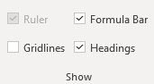
This will make your form look more like a form and less like a regular Excel sheet. Another thing you can do is in that same section, unselect the Formula Bar and Headings, which will add more white space and are unnecessary if someone is just filling in a form. However, you may want to save this for the end when your form is done.
Since an Excel form can come in all shapes and sizes, the one thing that may help you in the design process is to set every column to a width of 2. This way, it will be easier to maneuver in case one field needs to be bigger than another without having to try and force everything to be a similar length.
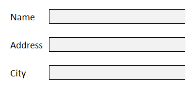
As for the input fields, there are a few things you will want to do:
- Make sure they are long enough. A good way to test this is by entering a long value, or what you might think will be the longest value into each field and then adjusting its length so that everything displays correctly.
- Assign a named range. This is useful to keep things organized and it will make it easier for you to refer back to the field later on if you only have to remember its name, as opposed to its cell reference.
Now, let’s move on to creating the fields in the Excel form. What you can do for text entries is to just add some outlining and highlighting to existing cells. A subtle light grey can be a good way to indicate that is an input value. And I’ll also add a border to help make these fields stand out. If you set the column width to 2, you’ll also need to merge the cells as needed.
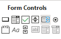
For the State field, I’ll go back to the Developer tab where I will select the option for a List Box from the Form Control section — which is next to the Radio Button on the right. When in doubt, you can hover over each control to see what it is.
After creating the List Box, I need to populate the list plus link to a cell where the selected value should go. I’ll start with creating a range of cells for all 50 states and then assign a named range for them called StateList.
Then, I will set up a named range called StateNumber for the linked cell. Here is what the List Box control shows when I go into Format Controls and select the Controls tab:
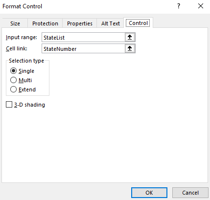
But this is not enough as the list box returns a number, not the state’s initials. I will need another cell to pull that in. I created a named range for State and here is what my sheet looks like:
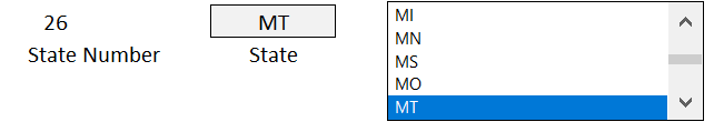
In the list box, I selected MT, which returns a value of 26 in the StateNumber range. To extract the state’s initials, I need to use a formula to get that. Since I’m getting the data from one column, I’m just going to use the INDEX function. Here is what the formula in the State named range looks like:
=INDEX(StateList,StateNumber,1)
It is looking at the StateList and pulling out the row that relates to the StateNumber. Since MT is the 26th selection, that is the value that gets returned. So now my List Box is working correctly. What I like to do with these named ranges is to hide them so that the user doesn’t see all these intermediate steps. All it takes is to just move the List Box over top of these cells:
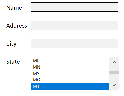
And just like that, the user only sees their selection and not the calculations afterwards. You could certainly use a drop-down list for states but I thought I would try something different and more user-friendly for this example.
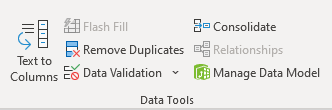
Next, let’s go to the email field. This can be tricky because although you want this to be text, you also want to control what a user enters to avoid a possible error. You can’t guarantee the email will be correct but you can take steps to at least prevent some errors. The key here is going to be to create a data validation rule. There are two things that should be present in email addresses: the @ sign and a period. To create a data validation rule, select on the cell and click on Data Validation under the Data tab:
There are many rules you can set up such as limiting the entry to fall within certain dates, making sure it is a whole number, or that it is from a drop-down list. But this situation is unique and will require a custom formula.
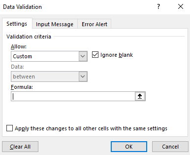
To check for both the period and the @ sign, I will need to use the FIND function and check that the value is a number (which means that it was found). Here’s how that looks inside of an AND function:
=AND(ISNUMBER(FIND(“.”,Email)),ISNUMBER(FIND(“@”,Email)))
Since I set the field to a named range of ‘Email’ it is easy to reference it without worrying about whether I have selected the right cell. If I put this calculation in the formula section, now you won’t be able to enter a value that doesn’t include both a period and an @ sign. In addition, you can also specify the error alert and determine what pops up if someone enters something different that violates these rules. However, that’s not necessary as they will get an error anyway.
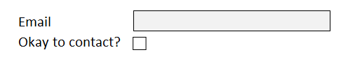
Now, I’ll add the checkbox for the email. This again comes from Excel’s Developer tab and the Form Control section. Simply select the checkbox and set up a linked cell. If you want more details on this, refer to the link at the top of this post for a more detailed outline of how to add checkboxes. I have positioned the checkbox right below the email field:
Next, I’ll add some radio buttons to allow someone to leave a rating. These are useful if you want to specify a number. Here I will go back to the Developer tab and create some radio buttons and re-size them so they don’t take up much space. Unlike the other controls, you will want them to all have the same linked cell; the purpose of radio buttons is that there is only one selection. Here is how I added them, just below the numbers that they refer to:

The radio buttons will automatically increment on their own so if you don’t pay attention to what order you’ve added them in you may get some unexpected results.
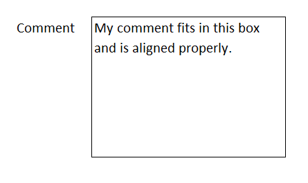
Lastly, I will add a large comment box where people can leave detailed comments. This can just be a large merged cell that takes up more space.
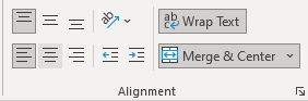
But the one thing you will want to do is make sure that Wrap Text is selected so that the comment fits in the box. And you will probably want to align it so that it is in the top left corner of the cell:
Then, when I enter the text it looks correct:
Here is what my completed form looks like:
It looks good, but we are still not done. Something needs to happen with these inputs otherwise the information goes nowhere. Let’s go over that next.
Step 3: Storing the data from the form in an Excel sheet
If you are sending just a single form over for someone to enter data in, what you can do is create an output page that will link to these values. Since they are all named ranges, you can easily reference back to them as such:
=Name
In the above example, if you created a named range called Name for the first field, it will pull in the data from there. On an output sheet, you might have formulas and values that look like this:
In column B I am showing the formulas. You can keep this tab hidden if you want it out of sight. You can even go one step further and make them very hidden.
Not sure whether your fields should go horizontally or vertically? In most cases, you’ll actually want them going across the top. When in doubt, consider the number of fields you have versus how much data you will be entering into the sheet. If you will have dozens of results that you will need to populate (or more), you probably don’t want to be cycling through that many columns; rows are easier to scroll through and that’s why it will probably make more sense for the fields to go across the top.
Once you have your output tab set up, you can copy the values you get back from these forms and start populating a database.
But what if you are doing data entry and need to make these entries multiple times and need the data to push to the output tab automatically after each entry? This is where you will need to set up a macro and need a button to trigger this movement onto the output tab. If you’d like to see how that code might work or just want a ready-to-use file that you don’t have to mess around with, you can download this free template.
The template will grab the input values and based on the named ranges, it will populate them in the output tab once you click the Post button on the main page. If there isn’t a named range that matches to a header on row 1 on the output tab, the data just won’t get copied over. Give it a try!
One additional step you may want to consider is locking down the form in Excel to make sure people don’t accidentally move things around or delete any formulas. You can protect the workbook and the individual sheets do that. Click here for information on how to lock cells.
If you liked this post on how to create a form in Excel, please give this site a like on Facebook and also be sure to check out some of the many templates that we have available for download. You can also follow us on Twitter and YouTube.

One of the ways in which Microsoft Forms is different than Google Forms, is that if you create a Form from the Forms web app, there is no Excel sheet attached.
This creates an extra step if you want to play with the data collected from a form.
Another difference is that when you do download that data it isn’t linked to the form, instead it’s a snapshot of the data at that time.
Well, fear not, if you want to have a spreadsheet that is collecting your data (and will continue to update in real time as new entries come in) you can. You just have to go a different route.
Microsoft makes it possible to create Forms right from an Excel spreadsheet. When you do this, it will link the spreadsheet to the form and continue to add the data.
Follow the steps below to make it so.
- Sign in to Office 365 with your school or work credentials.
- Open the Excel workbook in which you want to insert a form.
-
Click Insert > Forms > New Form to begin creating your form.
Note: To enable the Forms button, make sure your Excel workbook is stored in OneDrive for Business. Also note that Forms for Excel is only available for OneDrive for Business and new team sites connected with Office 365 groups. Learn more about Office 365 groups.
- A new tab, Microsoft Forms, will open.
- A default title for your form will be provided. To change it, click on the title and type a new name.
From here it should work just like a form created through the app. You can find the spreadsheet in OneDrive or through the Forms app.


Data Entry Forms is an extremely useful feature if inputting data is part of your daily work.
It can help you avoid the mistakes and make the data entry process faster. It also helps you focus on one record at a time!
It is a convenient and faster way to input records in Excel by displaying one row of information at a time without having to move from one column to another.
In this tutorial, we will show you How to Create Form in Excel for Data Entry.
Whenever I wanted to enter data in Excel, it would take me a very long time to input these records one by one, but I discovered a handy trick that can turn my Excel Table into a handy Excel Data Entry Form!

Say goodbye to inputting entering data into this Table row by row by row by row….
Below, we will cover the Top 11 Excel Data Entry Form Tips and Tricks that will be beneficial for you:
- #1 – Create Form in Excel
- #2 – Add to Quick Access Toolbar (QAT)
- #3 – Access the Form anytime
- #4 – Browse through Records
- #5 – Edit Existing Record
- #6 – Search Criteria
- #7 – Restore a Record
- #8 – Data Validation in Forms
- #9 – Delete a Record
- #10 – Close the Form
- #11 – Keyboard Shortcuts for Data Entry Forms
Make sure to download the Excel Workbook below and follow along:
DOWNLOAD EXCEL WORKBOOK
Want to know how to use the Data Entry Form?
*** Watch our video and step by step guide below with free downloadable Excel workbook to practice ***
Watch it on YouTube and give it a thumbs-up!
Watch it on YouTube and give it a thumbs-up!
Watch it on YouTube and give it a thumbs-up!
1. Create Form in Excel
I will show you how easy it is to Create Form in Excel for Data Entry with the following quick video below (scroll further down to see the step by step instructions after you watch this awesome video).
*** Watch our video below on How to Create Form in Excel in 5 minutes!***

DOWNLOAD OUR
FREE EXCEL GUIDES
In this tutorial, you have learned how to create form in Excel with minutes without using VBA!!
Follow the steps below:
STEP 1: Convert your Column names into a Table, go to Insert> Table
Make sure My table has headers is also checked.

STEP 2:Let us add the Form Creation functionality to understand how to make a fillable form in Excel.
Go to File > Options


STEP 3:Go to Customize Ribbon.
Select Commands Not in the Ribbon and Form. This is the functionality we need.
Click New Tab.

STEP 4:Under the New Tab, select New Group, and click Add.
This will add Forms to a New Tab in our Ribbon.

Notice that there is also a Rename button, you can use it to rename the New Tab and New Group into something more descriptive, like Form:

STEP 5:Select your Table, and on your new Form tab, select Form.

STEP 6: A new Form dialogue box will pop up!
Input your data into each section.
Click New to save it. Repeat this process for all the records you want to add.
Press Close to get out of this screen and see the data in your Excel Table.

You can now use this new form to continually input data into your Excel Table!

2. Add to Quick Access Toolbar (QAT)
Now that you have learned how to create form in Excel, lets put them on your QAT for easy access.
To add to the quick access toolbar, follow the steps below:
STEP 1: Click on the small arrow right next to QAT.

STEP 2: Click on More Commands from the dropdown list.

STEP 3: In the Excel Options dialog box, select All Commands from Choose commands from list.

STEP 4: Select Form from the list and then click on Add>>.

STEP 5: Form is now available in the Customize Quick Access Toolbar. Click OK.

Data Entry Form is now part of your Quick Access Toolbar.

3. Access the Form anytime
To access the Excel Data Entry Form, click on any cell in the table and click on the Form icon in Quick Access Toolbar.

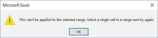
If you try to access the form when you haven’t selected a cell within the data table, you will receive an error message like the one shown below:

4. Browse through Records
To navigate through the existing records, simply use the Find Previous and Find Next buttons available on the Data Entry Form.

You can also use the scroll bar to go through the records one after the other.

This will save time when you have a data with multiple columns and records.
5. Edit Existing Record
Use the Find Previous and Find Next buttons to search for the record to want to edit.
Once you find the desired record, simply make the necessary edit and hit Enter in Excel.

The data table will be updated with the changes made.

6. Search Criteria
Using Wildcards
If you wish to search all entries containing the word “east” in the Region Column, you can do that by using the wildcard asterisk (*).
STEP 1: In the Data Entry Form, click on the Criteria button

STEP 2: In the Region field, type *east (to search all-region containing the word east)

STEP 3: Click Find Next to find the entries containing the word east.

Excel Data Entry Form will find the three entries for you in this scenario!


Using greater or less than sign
If you want to search for persons having a salary greater than or equal to $75,000, you can do so by following the steps below:
STEP 1: In the Data Entry Form, click on the Criteria button
STEP 2: In the Salary field, type >=75000.

STEP 3: Click Find Next to find all entries with a salary greater than or equal to $75,000.


7. Restore a Record
Suppose you have accidentally deleted the first name of a record.

And you don’t remember what was written in that field! Don’t panic.
You can use the Restore button in the Excel Data Entry Form and retrieve the data lost accidentally.

The data will reappear in the respective field.

One thing you need to keep in mind is that the Restore button is only useful if you haven’t hit Enter.
The moment you press the Enter button, the Restore button will become inactive and you won’t be able to revert back to the original data.
8. Data Validation in Forms
Even though you cannot directly add any data validation to the form. Any restriction created on the data table will still be in effect in the Forms.
Let’s see how!
Say, you add a list rule to the Region Column using Data Validation.
STEP 1: Select the Region Column.

STEP 2: Go to Data Tab > Data Tools (Group) > Data Validation.

STEP 3: In the Data Validation dialog box, click on the Allow dropdown and select List.

STEP 4: In the Source field, type Northeast, Northwest, Southeast, Southwest, and click OK.

Data Validation has now been inserted in the Region Column where you are only allowed to enter values present in the list (Northeast, Northwest, Southeast, Southwest).
STEP 5: Click on the Forms icon in QAT.

STEP 6: Change the Region for Record 1 from Northeast to East and Click OK.

Once you click OK, you will see an error message as below:

9. Delete a Record

STEP 1: Use the Scroll Bar to navigate to find the entry you want to delete.
STEP 2: Simply, click on the Delete button.

STEP 3: A confirmation message will appear on your screen, Click OK.

The desired entry will be removed from the data table.

10. Close the Form
To close the dialog box for Data Forms, simply click on the Close button (X) on the top-right corner of the bix.

11. Keyboards Shortcuts for Data Entry Forms
You can use the following keyboard shortcuts to work faster when using Data Entry Forms:
- Press Tab to go to the next field in the Excel Forms.
- Press Enter to go to the next record in the Excel Forms.
- Hit the Esc button on your keyboard to close the Excel Form.
This completes our tutorial on the Top 11 things you should know if Data Entry is what you do in Excel. It will not only make the process faster but also a lot more easier and fun!
Few things to keep in mind when using the Excel Data Entry Form are:
- You can add a maximum of 32 fields per record.
- You cannot print a data form record.
- Before you hit Enter, you can restore any changes made to the data.
So, give it a try! I am sure you are gonna love it!!
You can know more about How to Create Form in Excel by going through this tutorial by Microsoft.

Watch the Video on Using Data Entry Forms in Excel
Below is a detailed written tutorial about Excel Data Entry form in case you prefer reading over watching a video.
Excel has many useful features when it comes to data entry.
And one such feature is the Data Entry Form.
In this tutorial, I will show you what are data entry forms and how to create and use them in Excel.
Why Do You Need to Know About Data Entry Forms?
Maybe you don’t!
But if data entry is a part of your daily work, I recommend you check out this feature and see how it can help you save time (and make you more efficient).
There are two common issues that I have faced (and seen people face) when it comes to data entry in Excel:
- It’s time-consuming. You need to enter the data in one cell, then go to the next cell and enter the data for it. Sometimes, you need to scroll up and see which column it is and what data needs to be entered. Or scroll to the right and then come back to the beginning in case there are many columns.
- It’s error-prone. If you have a huge data set which needs 40 entries, there is a possibility you may end up entering something that was not intended for that cell.
A data entry form can help by making the process faster and less error-prone.
Before I show you how to create a data entry form in Excel, let me quickly show you what it does.
Below is a data set that is typically maintained by the hiring team in an organization.
Every time a user has to add a new record, he/she will have to select the cell in the next empty row and then go cell by cell to make the entry for each column.
While this is a perfectly fine way of doing it, a more efficient way would be to use a Data Entry Form in Excel.
Below is a data entry form that you can use to make entries to this data set.
The highlighted fields are where you would enter the data. Once done, hit the Enter key to make the data a part of the table and move on to the next entry.
Below is a demo of how it works:
As you can see, this is easier than regular data entry as it has everything in a single dialog box.
Data Entry Form in Excel
Using a data entry form in Excel needs a little pre-work.
You would notice that there is no option to use a data entry form in Excel (not in any tab in the ribbon).
To use it, you will have to first add it to the Quick Access Toolbar (or the ribbon).
Adding Data Entry Form Option To Quick Access Toolbar
Below are the steps to add the data entry form option to the Quick Access Toolbar:
- Right-click on any of the existing icons in the Quick Access Toolbar.
- Click on ‘Customize Quick Access Toolbar’.

- In the ‘Excel Options’ dialog box that opens, select the ‘All Commands’ option from the drop-down.

- Scroll down the list of commands and select ‘Form’.

- Click on the ‘Add’ button.

- Click OK.


The above steps would add the Form icon to the Quick Access Toolbar (as shown below).
![]()
Once you have it in QAT, you can click any cell in your dataset (in which you want to make the entry) and click on the Form icon.
Note: For Data Entry Form to work, your data should be in an Excel Table. If it isn’t already, you’ll have to convert it into an Excel Table (keyboard shortcut – Control + T).
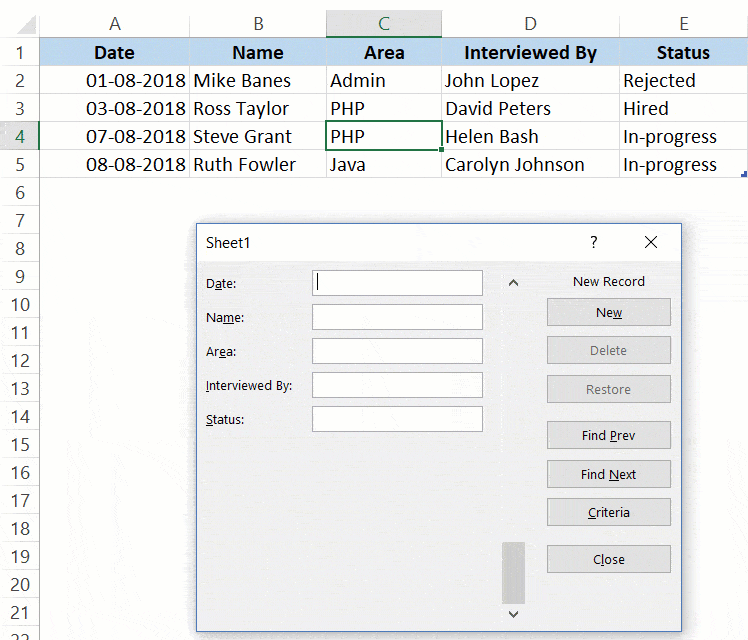
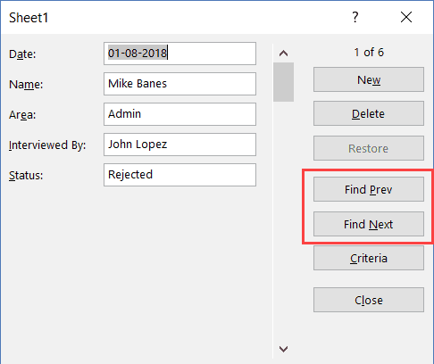
Parts of the Data Entry Form
A Data Entry Form in Excel has many different buttons (as you can see below).
Here is a brief description of what each button is about:
- New: This will clear any existing data in the form and allows you to create a new record.
- Delete: This will allow you to delete an existing record. For example, if I hit the Delete key in the above example, it will delete the record for Mike Banes.
- Restore: If you’re editing an existing entry, you can restore the previous data in the form (if you haven’t clicked New or hit Enter).
- Find Prev: This will find the previous entry.
- Find Next: This will find the next entry.
- Criteria: This allows you to find specific records. For example, if I am looking for all the records, where the candidate was Hired, I need to click the Criteria button, enter ‘Hired’ in the Status field and then use the find buttons. Example of this is covered later in this tutorial.
- Close: This will close the form.
- Scroll Bar: You can use the scroll bar to go through the records.
Now let’s go through all the things you can do with a Data Entry form in Excel.
Note that you need to convert your data into an Excel Table and select any cell in the table to be able to open the Data Entry form dialog box.
If you haven’t selected a cell in the Excel Table, it will show a prompt as shown below:
Creating a New Entry
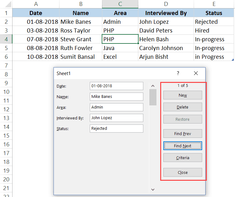
Below are the steps to create a new entry using the Data Entry Form in Excel:
- Select any cell in the Excel Table.
- Click on the Form icon in the Quick Access Toolbar.

- Enter the data in the form fields.
- Hit the Enter key (or click the New button) to enter the record in the table and get a blank form for next record.
Navigating Through Existing Records
One of the benefits of using Data Entry Form is that you can easily navigate and edit the records without ever leaving the dialog box.
This can be especially useful if you have a dataset with many columns. This can save you a lot of scrolling and the process of going back and forth.
Below are the steps to navigate and edit the records using a data entry form:
- Select any cell in the Excel Table.
- Click on the Form icon in the Quick Access Toolbar.
- To go to the next entry, click on the ‘Find Next’ button and to go to the previous entry, click the ‘Find Prev’ button.

- To edit an entry, simply make the change and hit enter. In case you want to revert to the original entry (if you haven’t hit the enter key), click the ‘Restore’ button.
You can also use the scroll bar to navigate through entries one-by-one.
The above snapshot shows basic navigation where you are going through all the records one after the other.
But you can also quickly navigate through all the records based on criteria.
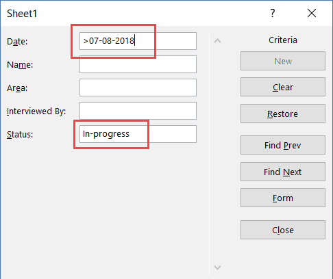
For example, if you want to go through all the entries where the status is ‘In-progress’, you can do that using the below steps:
Criteria is a very useful feature when you have a huge dataset, and you want to quickly go through those records that meet a given set of criteria.
Note that you can use multiple criteria fields to navigate through the data.
For example, if you want to go through all the ‘In-progress’ records after 07-08-2018, you can use ‘>07-08-2018’ in the criteria for ‘Date’ field and ‘In-progress’ as the value in the status field. Now when you navigate using Find Prev/Find Next buttons, it will only show records after 07-08-2018 where the status is In-progress.
You can also use wildcard characters in criteria.
For example, if you have been inconsistent in entering the data and have used variations of a word (such as In progress, in-progress, in progress, and inprogress), then you need to use wildcard characters to get these records.
Below are the steps to do this:
- Select any cell in the Excel table.
- Click on the Form icon in the Quick Access Toolbar.
- Click the Criteria button.
- In the Status field, enter *progress
- Use the Find Prev/Find Next buttons to navigate through the entries where the status is In-Progress.

This works as an asterisk (*) is a wildcard character that can represent any number of characters in Excel. So if the status contains the ‘progress’, it will be picked up by Find Prev/Find Next buttons no matter what is before it).
Deleting a Record
You can delete records from the Data Entry form itself.
This can be useful when you want to find a specific type of records and delete these.
Below are the steps to delete a record using Data Entry Form:
- Select any cell in the Excel table.
- Click on the Form icon in the Quick Access Toolbar.
- Navigate to the record you want to delete
- Click the Delete button.

While you may feel that this all looks like a lot of work just to enter and navigate through records, it saves a lot of time if you’re working with lots of data and have to do data entry quite often.
Restricting Data Entry Based on Rules
You can use data validation in cells to make sure the data entered conforms to a few rules.
For example, if you want to make sure that the date column only accepts a date during data entry, you can create a data validation rule to only allow dates.
If a user enters a data that is not a date, it will not be allowed and the user will be shown an error.
Here is how to create these rules when doing data entry:
- Select the cells (or even the entire column) where you want to create a data validation rule. In this example, I have selected column A.
- Click the Data tab.

- Click the Data Validation option.

- In the ‘Data Validation’ dialog box, within the ‘Settings’ tab, select ‘Date’ from the ‘Allow’ drop down.

- Specify the start and the end date. Entries within this date range would be valid and rest all would be denied.
- Click OK.


Now, if you use the data entry form to enter data in the Date column, and if it isn’t a date, then it will not be allowed.
You will see a message as shown below:
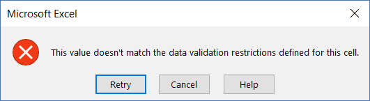
Similarly, you can use data validation with data entry forms to make sure users don’t end up entering the wrong data. Some examples where you can use this is numbers, text length, dates, etc.
Here are a few important things to know about Excel Data Entry Form:
- You can use wildcard characters while navigating through the records (through criteria option).
- You need to have an Excel table to be able to use the Data Entry Form. Also, you need to have a cell selected in it to use the form. There is one exception to this though. If you have a named range with the name ‘Database’, then the Excel Form will also refer to this named range, even if you have an Excel table.
- The field width in the Data Entry form is dependent on the column width of the data. If your column width is too narrow, the same would be reflected in the form.
- You can also insert bullet points in the data entry form. To do this, use the keyboard shortcut ALT + 7 or ALT + 9 from your numeric keypad. Here is a video about bullet points.
You May Also Like the Following Excel Tutorials:
- 100+ Excel Interview Questions.
- Drop Down Lists in Excel.
- Find and Remove Duplicates in Excel.
- Excel Text to Columns.