
For quick access to related information in another file or on a web page, you can insert a hyperlink in a worksheet cell. You can also insert links in specific chart elements.
Note: Most of the screen shots in this article were taken in Excel 2016. If you have a different version your view might be slightly different, but unless otherwise noted, the functionality is the same.
-
On a worksheet, click the cell where you want to create a link.
You can also select an object, such as a picture or an element in a chart, that you want to use to represent the link.
-
On the Insert tab, in the Links group, click Link
 .
.
You can also right-click the cell or graphic and then click Link on the shortcut menu, or you can press Ctrl+K.
-
-
Under Link to, click Create New Document.
-
In the Name of new document box, type a name for the new file.
Tip: To specify a location other than the one shown under Full path, you can type the new location preceding the name in the Name of new document box, or you can click Change to select the location that you want and then click OK.
-
Under When to edit, click Edit the new document later or Edit the new document now to specify when you want to open the new file for editing.
-
In the Text to display box, type the text that you want to use to represent the link.
-
To display helpful information when you rest the pointer on the link, click ScreenTip, type the text that you want in the ScreenTip text box, and then click OK.
 .
.-
On a worksheet, click the cell where you want to create a link.
You can also select an object, such as a picture or an element in a chart, that you want to use to represent the link.
-
On the Insert tab, in the Links group, click Link
.
You can also right-click the cell or object and then click Link on the shortcut menu, or you can press Ctrl+K.
-
-
Under Link to, click Existing File or Web Page.
-
Do one of the following:
-
To select a file, click Current Folder, and then click the file that you want to link to.
You can change the current folder by selecting a different folder in the Look in list.
-
To select a web page, click Browsed Pages and then click the web page that you want to link to.
-
To select a file that you recently used, click Recent Files, and then click the file that you want to link to.
-
To enter the name and location of a known file or web page that you want to link to, type that information in the Address box.
-
To locate a web page, click Browse the Web
, open the web page that you want to link to, and then switch back to Excel without closing your browser.
-
-
If you want to create a link to a specific location in the file or on the web page, click Bookmark, and then double-click the bookmark that you want.
Note: The file or web page that you are linking to must have a bookmark.
-
In the Text to display box, type the text that you want to use to represent the link.
-
To display helpful information when you rest the pointer on the link, click ScreenTip, type the text that you want in the ScreenTip text box, and then click OK.
 , open the web page that you want to link to, and then switch back to Excel without closing your browser.
To link to a location in the current workbook or another workbook, you can either define a name for the destination cells or use a cell reference.
-
To use a name, you must name the destination cells in the destination workbook.
How to name a cell or a range of cells
-
Select the cell, range of cells, or nonadjacent selections that you want to name.
-
Click the Name box at the left end of the formula bar
.
Name box -
In the Name box, type the name for the cells, and then press Enter.
Note: Names can’t contain spaces and must begin with a letter.
-
-
On a worksheet of the source workbook, click the cell where you want to create a link.
You can also select an object, such as a picture or an element in a chart, that you want to use to represent the link.
-
On the Insert tab, in the Links group, click Link
.
You can also right-click the cell or object and then click Link on the shortcut menu, or you can press Ctrl+K.
-
-
Under Link to, do one of the following:
-
To link to a location in your current workbook, click Place in This Document.
-
To link to a location in another workbook, click Existing File or Web Page, locate and select the workbook that you want to link to, and then click Bookmark.
-
-
Do one of the following:
-
In the Or select a place in this document box, under Cell Reference, click the worksheet that you want to link to, type the cell reference in the Type in the cell reference box, and then click OK.
-
In the list under Defined Names, click the name that represents the cells that you want to link to, and then click OK.
-
-
In the Text to display box, type the text that you want to use to represent the link.
-
To display helpful information when you rest the pointer on the link, click ScreenTip, type the text that you want in the ScreenTip text box, and then click OK.
 .
.
 Name box
You can use the HYPERLINK function to create a link that opens a document that is stored on a network server, an intranet, or the Internet. When you click the cell that contains the HYPERLINK function, Excel opens the file that is stored at the location of the link.
Syntax
HYPERLINK(link_location,friendly_name)
Link_location is the path and file name to the document to be opened as text. Link_location can refer to a place in a document — such as a specific cell or named range in an Excel worksheet or workbook, or to a bookmark in a Microsoft Word document. The path can be to a file stored on a hard disk drive, or the path can be a universal naming convention (UNC) path on a server (in Microsoft Excel for Windows) or a Uniform Resource Locator (URL) path on the Internet or an intranet.
-
Link_location can be a text string enclosed in quotation marks or a cell that contains the link as a text string.
-
If the jump specified in link_location does not exist or can’t be navigated, an error appears when you click the cell.
Friendly_name is the jump text or numeric value that is displayed in the cell. Friendly_name is displayed in blue and is underlined. If friendly_name is omitted, the cell displays the link_location as the jump text.
-
Friendly_name can be a value, a text string, a name, or a cell that contains the jump text or value.
-
If friendly_name returns an error value (for example, #VALUE!), the cell displays the error instead of the jump text.
Examples
The following example opens a worksheet named Budget Report.xls that is stored on the Internet at the location named example.microsoft.com/report and displays the text «Click for report»:
=HYPERLINK(«http://example.microsoft.com/report/budget report.xls», «Click for report»)
The following example creates a link to cell F10 on the worksheet named Annual in the workbook Budget Report.xls, which is stored on the Internet at the location named example.microsoft.com/report. The cell on the worksheet that contains the link displays the contents of cell D1 as the jump text:
=HYPERLINK(«[http://example.microsoft.com/report/budget report.xls]Annual!F10», D1)
The following example creates a link to the range named DeptTotal on the worksheet named First Quarter in the workbook Budget Report.xls, which is stored on the Internet at the location named example.microsoft.com/report. The cell on the worksheet that contains the link displays the text «Click to see First Quarter Department Total»:
=HYPERLINK(«[http://example.microsoft.com/report/budget report.xls]First Quarter!DeptTotal», «Click to see First Quarter Department Total»)
To create a link to a specific location in a Microsoft Word document, you must use a bookmark to define the location you want to jump to in the document. The following example creates a link to the bookmark named QrtlyProfits in the document named Annual Report.doc located at example.microsoft.com:
=HYPERLINK(«[http://example.microsoft.com/Annual Report.doc]QrtlyProfits», «Quarterly Profit Report»)
In Excel for Windows, the following example displays the contents of cell D5 as the jump text in the cell and opens the file named 1stqtr.xls, which is stored on the server named FINANCE in the Statements share. This example uses a UNC path:
=HYPERLINK(«\FINANCEStatements1stqtr.xls», D5)
The following example opens the file 1stqtr.xls in Excel for Windows that is stored in a directory named Finance on drive D, and displays the numeric value stored in cell H10:
=HYPERLINK(«D:FINANCE1stqtr.xls», H10)
In Excel for Windows, the following example creates a link to the area named Totals in another (external) workbook, Mybook.xls:
=HYPERLINK(«[C:My DocumentsMybook.xls]Totals»)
In Microsoft Excel for the Macintosh, the following example displays «Click here» in the cell and opens the file named First Quarter that is stored in a folder named Budget Reports on the hard drive named Macintosh HD:
=HYPERLINK(«Macintosh HD:Budget Reports:First Quarter», «Click here»)
You can create links within a worksheet to jump from one cell to another cell. For example, if the active worksheet is the sheet named June in the workbook named Budget, the following formula creates a link to cell E56. The link text itself is the value in cell E56.
=HYPERLINK(«[Budget]June!E56», E56)
To jump to a different sheet in the same workbook, change the name of the sheet in the link. In the previous example, to create a link to cell E56 on the September sheet, change the word «June» to «September.»
When you click a link to an email address, your email program automatically starts and creates an email message with the correct address in the To box, provided that you have an email program installed.
-
On a worksheet, click the cell where you want to create a link.
You can also select an object, such as a picture or an element in a chart, that you want to use to represent the link.
-
On the Insert tab, in the Links group, click Link
.
You can also right-click the cell or object and then click Link on the shortcut menu, or you can press Ctrl+K.
-
-
Under Link to, click E-mail Address.
-
In the E-mail address box, type the email address that you want.
-
In the Subject box, type the subject of the email message.
Note: Some web browsers and email programs may not recognize the subject line.
-
In the Text to display box, type the text that you want to use to represent the link.
-
To display helpful information when you rest the pointer on the link, click ScreenTip, type the text that you want in the ScreenTip text box, and then click OK.
You can also create a link to an email address in a cell by typing the address directly in the cell. For example, a link is created automatically when you type an email address, such as someone@example.com.
You can insert one or more external reference (also called links) from a workbook to another workbook that is located on your intranet or on the Internet. The workbook must not be saved as an HTML file.
-
Open the source workbook and select the cell or cell range that you want to copy.
-
On the Home tab, in the Clipboard group, click Copy.
-
Switch to the worksheet that you want to place the information in, and then click the cell where you want the information to appear.
-
On the Home tab, in the Clipboard group, click Paste Special.
-
Click Paste Link.
Excel creates an external reference link for the cell or each cell in the cell range.

Note: You may find it more convenient to create an external reference link without opening the workbook on the web. For each cell in the destination workbook where you want the external reference link, click the cell, and then type an equal sign (=), the URL address, and the location in the workbook. For example:
=’http://www.someones.homepage/[file.xls]Sheet1′!A1
=’ftp.server.somewhere/file.xls’!MyNamedCell
To select a hyperlink without activating the link to its destination, do one of the following:
-
Click the cell that contains the link, hold the mouse button until the pointer becomes a cross
, and then release the mouse button. -
Use the arrow keys to select the cell that contains the link.
-
If the link is represented by a graphic, hold down Ctrl, and then click the graphic.
 , and then release the mouse button.
You can change an existing link in your workbook by changing its destination, its appearance, or the text or graphic that is used to represent it.
Change the destination of a link
-
Select the cell or graphic that contains the link that you want to change.
Tip: To select a cell that contains a link without going to the link destination, click the cell and hold the mouse button until the pointer becomes a cross
, and then release the mouse button. You can also use the arrow keys to select the cell. To select a graphic, hold down Ctrl and click the graphic.-
On the Insert tab, in the Links group, click Link.
You can also right-click the cell or graphic and then click Edit Link on the shortcut menu, or you can press Ctrl+K.
-
-
In the Edit Hyperlink dialog box, make the changes that you want.
Note: If the link was created by using the HYPERLINK worksheet function, you must edit the formula to change the destination. Select the cell that contains the link, and then click the formula bar to edit the formula.
You can change the appearance of all link text in the current workbook by changing the cell style for links.
-
On the Home tab, in the Styles group, click Cell Styles.
-
Under Data and Model, do the following:
-
To change the appearance of links that have not been clicked to go to their destinations, right-click Link, and then click Modify.
-
To change the appearance of links that have been clicked to go to their destinations, right-click Followed Link, and then click Modify.
Note: The Link cell style is available only when the workbook contains a link. The Followed Link cell style is available only when the workbook contains a link that has been clicked.
-
-
In the Style dialog box, click Format.
-
On the Font tab and Fill tab, select the formatting options that you want, and then click OK.
Notes:
-
The options that you select in the Format Cells dialog box appear as selected under Style includes in the Style dialog box. You can clear the check boxes for any options that you don’t want to apply.
-
Changes that you make to the Link and Followed Link cell styles apply to all links in the current workbook. You can’t change the appearance of individual links.
-
-
Select the cell or graphic that contains the link that you want to change.
Tip: To select a cell that contains a link without going to the link destination, click the cell and hold the mouse button until the pointer becomes a cross
, and then release the mouse button. You can also use the arrow keys to select the cell. To select a graphic, hold down Ctrl and click the graphic. -
Do one or more of the following:
-
To change the link text, click in the formula bar, and then edit the text.
-
To change the format of a graphic, right-click it, and then click the option that you need to change its format.
-
To change text in a graphic, double-click the selected graphic, and then make the changes that you want.
-
To change the graphic that represents the link, insert a new graphic, make it a link with the same destination, and then delete the old graphic and link.
-
-
Right-click the hyperlink that you want to copy or move, and then click Copy or Cut on the shortcut menu.
-
Right-click the cell that you want to copy or move the link to, and then click Paste on the shortcut menu.
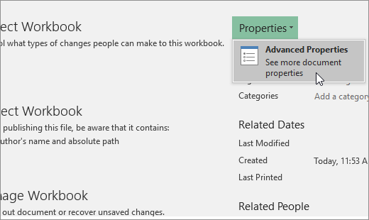
By default, unspecified paths to hyperlink destination files are relative to the location of the active workbook. Use this procedure when you want to set a different default path. Each time that you create a link to a file in that location, you only have to specify the file name, not the path, in the Insert Hyperlink dialog box.
Follow one of the steps depending on the Excel version you are using:
-
In Excel 2016, Excel 2013, and Excel 2010:
-
Click the File tab.
-
Click Info.
-
Click Properties, and then select Advanced Properties.
-
In the Summary tab, in the Hyperlink base text box, type the path that you want to use.
Note: You can override the link base address by using the full, or absolute, address for the link in the Insert Hyperlink dialog box.
-
-
In Excel 2007:
-
Click the Microsoft Office Button
, click Prepare, and then click Properties. -
In the Document Information Panel, click Properties, and then click Advanced Properties.
-
Click the Summary tab.
-
In the Hyperlink base box, type the path that you want to use.
Note: You can override the link base address by using the full, or absolute, address for the link in the Insert Hyperlink dialog box.
-
 , click Prepare, and then click Properties.
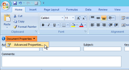
To delete a link, do one of the following:
-
To delete a link and the text that represents it, right-click the cell that contains the link, and then click Clear Contents on the shortcut menu.
-
To delete a link and the graphic that represents it, hold down Ctrl and click the graphic, and then press Delete.
-
To turn off a single link, right-click the link, and then click Remove Link on the shortcut menu.
-
To turn off several links at once, do the following:
-
In a blank cell, type the number 1.
-
Right-click the cell, and then click Copy on the shortcut menu.
-
Hold down Ctrl and select each link that you want to turn off.
Tip: To select a cell that has a link in it without going to the link destination, click the cell and hold the mouse button until the pointer becomes a cross
, and then release the mouse button. -
On the Home tab, in the Clipboard group, click the arrow below Paste, and then click Paste Special.
-
Under Operation, click Multiply, and then click OK.
-
On the Home tab, in the Styles group, click Cell Styles.
-
Under Good, Bad, and Neutral, select Normal.
-
A link opens another page or file when you click it. The destination is frequently another web page, but it can also be a picture, or an email address, or a program. The link itself can be text or a picture.
When a site user clicks the link, the destination is shown in a Web browser, opened, or run, depending on the type of destination. For example, a link to a page shows the page in the web browser, and a link to an AVI file opens the file in a media player.
How links are used
You can use links to do the following:
-
Navigate to a file or web page on a network, intranet, or Internet
-
Navigate to a file or web page that you plan to create in the future
-
Send an email message
-
Start a file transfer, such as downloading or an FTP process
When you point to text or a picture that contains a link, the pointer becomes a hand  , indicating that the text or picture is something that you can click.
What a URL is and how it works
When you create a link, its destination is encoded as a Uniform Resource Locator (URL), such as:
http://example.microsoft.com/news.htm
file://ComputerName/SharedFolder/FileName.htm
A URL contains a protocol, such as HTTP, FTP, or FILE, a Web server or network location, and a path and file name. The following illustration defines the parts of the URL:
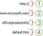
1. Protocol used (http, ftp, file)
2. Web server or network location
3. Path
4. File name
Absolute and relative links
An absolute URL contains a full address, including the protocol, the Web server, and the path and file name.
A relative URL has one or more missing parts. The missing information is taken from the page that contains the URL. For example, if the protocol and web server are missing, the web browser uses the protocol and domain, such as .com, .org, or .edu, of the current page.
It is common for pages on the web to use relative URLs that contain only a partial path and file name. If the files are moved to another server, any links will continue to work as long as the relative positions of the pages remain unchanged. For example, a link on Products.htm points to a page named apple.htm in a folder named Food; if both pages are moved to a folder named Food on a different server, the URL in the link will still be correct.
In an Excel workbook, unspecified paths to link destination files are by default relative to the location of the active workbook. You can set a different base address to use by default so that each time that you create a link to a file in that location, you only have to specify the file name, not the path, in the Insert Hyperlink dialog box.
-
On a worksheet, select the cell where you want to create a link.
-
On the Insert tab, select Hyperlink.
You can also right-click the cell and then select Hyperlink… on the shortcut menu, or you can press Ctrl+K.
-
Under Display Text:, type the text that you want to use to represent the link.
-
Under URL:, type the complete Uniform Resource Locator (URL) of the webpage you want to link to.
-
Select OK.
To link to a location in the current workbook, you can either define a name for the destination cells or use a cell reference.
-
To use a name, you must name the destination cells in the workbook.
How to define a name for a cell or a range of cells
Note: In Excel for the Web, you can’t create named ranges. You can only select an existing named range from the Named Ranges control. Alternately, you can open the file in the Excel desktop app, create a named range there, and then access this option from Excel for the web.
-
Select the cell or range of cells that you want to name.
-
On the Name Box box at the left end of the formula bar
, type the name for the cells, and then press Enter.Note: Names can’t contain spaces and must begin with a letter.
-
-
On the worksheet, select the cell where you want to create a link.
-
On the Insert tab, select Hyperlink.
You can also right-click the cell and then select Hyperlink… on the shortcut menu, or you can press Ctrl+K.
-
Under Display Text:, type the text that you want to use to represent the link.
-
Under Place in this document:, enter the defined name or cell reference.
-
Select OK.
When you click a link to an email address, your email program automatically starts and creates an email message with the correct address in the To box, provided that you have an email program installed.
-
On a worksheet, select the cell where you want to create a link.
-
On the Insert tab, select Hyperlink.
You can also right-click the cell and then select Hyperlink… on the shortcut menu, or you can press Ctrl+K.
-
Under Display Text:, type the text that you want to use to represent the link.
-
Under E-mail address:, type the email address that you want.
-
Select OK.
You can also create a link to an email address in a cell by typing the address directly in the cell. For example, a link is created automatically when you type an email address, such as someone@example.com.
You can use the HYPERLINK function to create a link to a URL.
Note: The Link_location can be a text string enclosed in quotation marks or a reference to a cell that contains the link as a text string.
To select a hyperlink without activating the link to its destination, do any of the following:
-
Select a cell by clicking it when the pointer is an arrow.
-
Use the arrow keys to select the cell that contains the link.
You can change an existing link in your workbook by changing its destination, its appearance, or the text that is used to represent it.
-
Select the cell that contains the link that you want to change.
Tip: To select a hyperlink without activating the link to its destination, use the arrow keys to select the cell that contains the link.
-
On the Insert tab, select Hyperlink.
You can also right-click the cell or graphic and then select Edit Hyperlink… on the shortcut menu, or you can press Ctrl+K.
-
In the Edit Hyperlink dialog box, make the changes that you want.
Note: If the link was created by using the HYPERLINK worksheet function, you must edit the formula to change the destination. Select the cell that contains the link, and then select the formula bar to edit the formula.
-
Right-click the hyperlink that you want to copy or move, and then select Copy or Cut on the shortcut menu.
-
Right-click the cell that you want to copy or move the link to, and then select Paste on the shortcut menu.
To delete a link, do one of the following:
-
To delete a link, select the cell and press Delete.
-
To turn off a link (delete the link but keep the text that represents it), right-click the cell and then select Remove Hyperlink.
Need more help?
You can always ask an expert in the Excel Tech Community or get support in the Answers community.
See Also
Remove or turn off links
![]()
Download Article
![]()
Download Article
This wikiHow teaches you how to link data between multiple worksheets in a Microsoft Excel workbook. Linking will dynamically pull data from a sheet into another, and update the data in your destination sheet whenever you change the contents of a cell in your source sheet.
Steps
-
1
Open a Microsoft Excel workbook. The Excel icon looks like a green-and-white «X» icon.
-
2
Click your destination sheet from the sheet tabs. You will see a list of all your worksheets at the bottom of Excel. Click on the sheet you want to link to another worksheet.
Advertisement
-
3
Click an empty cell in your destination sheet. This will be your destination cell. When you link it to another sheet, the data in this cell will be automatically synchronized and updated whenever the data in your source cell changes.
-
4
Type = in the cell. It will start a formula in your destination cell.
-
5
Click your source sheet from the sheet tabs. Find the sheet where you want to pull data from, and click on the tab to open the worksheet.
-
6
Check the formula bar. The formula bar shows the value of your destination cell at the top of your workbook. When you switch to your source sheet, it should show the name of your current worksheet, following an equals sign, and followed by an exclamation mark.
- Alternatively, you can manually write this formula in the formula bar. It should look like =<SheetName>!, where «<SheetName>» is replaced with the name of your source sheet.
-
7
Click a cell in your source sheet. This will be your source cell. It could be an empty cell, or a cell with some data in it. When you link sheets, your destination cell will be automatically updated with the data in your source cell.
- For example, if you’re pulling data from cell D12 in Sheet1, the formula should look like =Sheet1!D12.
-
8
Click ↵ Enter on your keyboard. This will finalize the formula, and switch back to your destination sheet. Your destination cell is now linked to your source cell, and dynamically pulls data from it. Whenever you edit the data in your source cell, your destination cell will also be updated.
-
9
Click your destination cell. This will highlight the cell.
-
10
Click and drag the square icon in the lower-right corner of your destination cell. This will expand the range of linked cells between your source and destination sheets. Expanding your initial destination cell will link the adjacent cells from your source sheet.
- You can drag and expand the range of linked cells in any direction. This could include the entire worksheet, or only parts of it.


Advertisement
Ask a Question
200 characters left
Include your email address to get a message when this question is answered.
Submit
Advertisement
Thanks for submitting a tip for review!
About This Article
Article SummaryX
1. Open Excel.
2. Click your destination cell.
3. Type «=«.
4. Click another sheet.
5. Click your source cell.
6. Press Enter on your keyboard.
Did this summary help you?
Thanks to all authors for creating a page that has been read 335,103 times.
Is this article up to date?
Excel files are also called workbooks for a very good reason. They can have multiple sheets, or worksheets, to help you organize your data. When working with multiple sheets, you may need to have links between them so that values in one sheet can be used in another.
In this article, we’ll explain how to link data between worksheets in Excel. You’ll see several examples on linking sheets in the same workbook as well as across different ones.
Why link data between sheets in Excel?
Linking sheets in Excel can be a great way to organize your data and keep them consistent across different worksheets. You may want to do this for different purposes, for example:
- You have a workbook containing data split by month, by state, or by salesperson, and you want a summary in one of the sheets.
- You want to create lists using links from different sheets in Excel.
- You want to collect data from multiple sheets and combine them into one to create a master sheet. Or, you may want to link data from a master sheet so that your data in other sheets are always up-to-date.
- Your data is growing and becoming too voluminous. As a result, you split it into different workbooks to be managed by different people. There can be times when you need to write formulas to get data out of these files.
Creating links between sheets is pretty easy to do. Besides, the main benefit is that whenever your data in the source sheet changes, the data in the destination sheet will be automatically updated as well.
Problems with linking large data between worksheets in the same or different Excel workbooks
Indeed, using multiple worksheets can certainly make your data in one workbook easier to manage. However, linking large amounts of data between worksheets could decrease the performance of your Excel workbook. Avoid inter-workbook links unless it’s absolutely necessary because they can be slow, easily broken, and not always easy to find and fix.
We suggest you try another solution 👇
When getting large data from different worksheets, especially from different workbooks, we recommend that you import instead of linking. Linking will slow down your Excel file, while an optimized performance can be maintained if you simply import data from Excel to Excel. Use a tool such as Coupler.io to refresh your data on the schedule you want to keep your data up-to-date.

To start using Coupler.io, sign up for a free account and create your first importer. A wizard will walk you through setting up the source, destination, and auto-refresh schedule for your importer. If you’re importing from Excel to Excel, choose Microsoft Excel as the source and destination of your importer, as follows:
#1. Set up a source
Select Microsoft Excel as the source that contains your data. You’ll need to connect to your Microsoft account and select the workbook and worksheet(s) you want to import. If you want, you can import only a selected range from your worksheets, e.g., range B3:G10 only.

Notice that with Coupler.io, you can also import data from different sources such as HubSpot, Jira, QuickBooks, and more. Check out the complete list of Coupler.io integrations with Excel.
#2. Set up a destination
For the destination, select Microsoft Excel. No need to connect again if you’re importing to the same Microsoft account. After that, choose the workbook and worksheet where you want your data imported.

#3. Schedule
You can keep your data up-to-date by setting up an automatic data refresh on the schedule you want.

Finally, click Save and Run to run your first importer. The import process may take several seconds or minutes to complete.
How to link two Excel sheets in the same workbook
Now, let’s see how to link two sheets in the same Excel workbook, including some tips and examples.
How to link sheets in Excel with a formula
To refer to a cell or range in another worksheet in the same workbook, type the name of the source worksheet followed by an exclamation mark (!) before the range address—see the following examples:
- To reference a single cell A1 in Sheet2:
=Sheet2!A1
- To reference a single cell A1 but the sheet name contains spaces:
='Sheet 2'!A1
- To reference a range of cells A1 to C10 in Sheet2:
=Sheet2!A1:C10
- To reference column A in Sheet2:
=Sheet2!A:A
- To reference multiple columns A to E in Sheet2:
=Sheet2!A:E
- To reference row 5 in Sheet2:
=Sheet2!5:5
- To reference multiple rows 1 to 5 in Sheet2:
=Sheet2!1:5
- To reference a worksheet-level named range Data in Sheet2:
=Sheet2!Data
- To reference a workbook-level named range Data in Sheet2:
=Data
You can always manually type the linking formula in a destination cell. However, doing that is not recommended because it typically leads to mistakes. So, instead of typing the formula manually, check the tips below.
Tip 1: Create a link from the destination sheet
With the following spreadsheet, suppose you want to show the total for New York in the Summary sheet. In cell B2 of the Summary sheet, you want to display the values of cell F5 from the New York sheet.
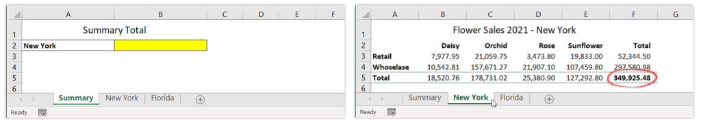
To do that, follow the steps below:
- Begin by opening the destination sheet (Summary).
- Type = (equal sign) in the destination cell (B2).

- Switch to source sheet (New York).
- Select the cell you want to link (F5), then press Enter.

As a result, when you click on the destination cell, you’ll see the following formula:
='New York'!F5

Notice that Excel automatically encloses the sheet name with single quotation marks because there is a space character in the sheet name.
Tip 2: Use Copy and Paste Link
This second tip also allows you to link to another sheet without manually typing the linking formula. Unlike the first method that begins from the destination sheet, this method starts from the source sheet.
This time, suppose you want to show the total for Florida in the Summary sheet. In cell B3 of the Summary sheet, you want to display the values of cell F5 from the Florida sheet.

Follow the steps below:
- Begin by opening the source sheet (Florida).
- Right-click on the cell you want to link (F5), then select Copy.
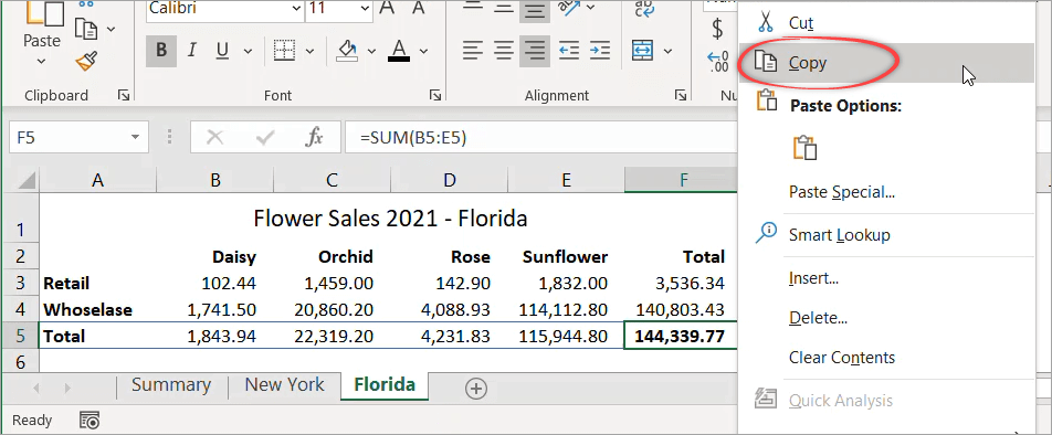
- Switch to the destination sheet (Summary).
- In the destination cell (B3), right-click and select Paste Link.

As a result, when you click on B3, you’ll see the following formula:
=Florida!$F$5

Notice that by default, this method returns an absolute reference. If you want to change it to a relative reference, simply highlight the formula and press F4 multiple times to remove the dollar signs.
How to link numbers from different sheets in Excel using the INDIRECT function
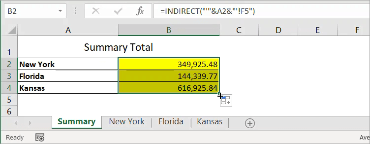
In the previous example, notice that the New York and Florida sheets have the same layout. In cases like this, you can also use the INDIRECT function in the formula to get the totals.
Now, let’s see the following spreadsheet with a Summary sheet and three other sheets with a similar layout. Assume you want to link the total in cell F5 from the three sheets and put them in the Summary sheet using the INDIRECT function.

To do that, follow the steps below:
- Link the total for New York only:
='New York'!F5

- Replace the formula using the INDIRECT function below. Notice that we concatenate A2 with single quotes because its value contains a space character.
=INDIRECT("'"&A2&"'!F5")

- Drag the formula down to A4 to apply it to the other states.
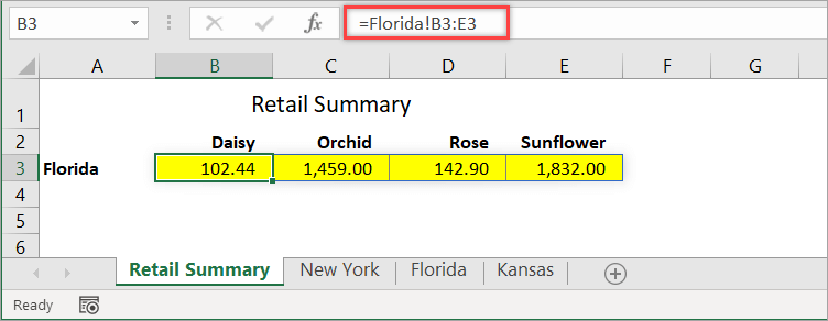
How to link data in a range of cells between sheets in Excel
With the following spreadsheet, suppose you want to link the retail sales data for Florida and put them in the Retail Summary sheet, as the following screenshot shows:

The range to link is in B3:E3 of the second sheet. To display it in the destination sheet, use the following formula in a cell:
=Florida!B3:E3
How to link columns from different sheets to another sheet in Excel
With the following spreadsheet, suppose you want to link the entire Column B from the Product sheet to Sheet1. To do that, you can use the following formula:
=Product!B:B

However, if you notice, the blank cells are showing zeros. If you want to see empty cells when there is nothing in the original sheet, you can change the formula to the one below:
=IF(LEN(Product!B:B)>0, Product!B:B,"")

How to link to a defined name in other sheets in Excel
For most people, words are easier to remember than numbers or codes. For this reason, Excel allows you to name an individual cell or range of cells. Then, you can use these names when referring to data in another sheet instead of typing the range address.
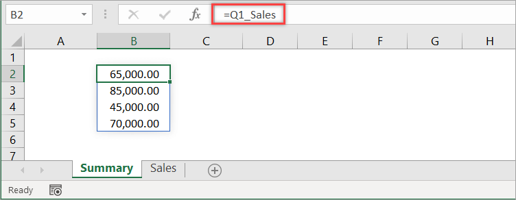
With the following worksheet, let’s create a defined name for range B2:B5 and name it Q1_Sales.
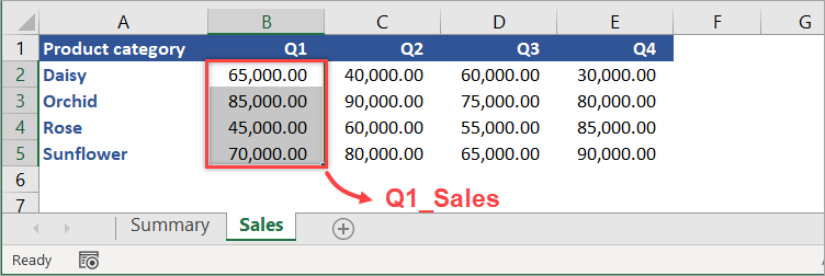
First, select the range of cells to include (B2:B5). Then, in the Name Box, type Q1_Sales and press Enter — and Done!

By default, Excel creates the name at the workbook level. To reference the defined name in another worksheet, just type the following formula into any cell.
=Q1_Sales
You can also use the defined name with an Excel function in a formula. For example, the following formula calculates the average of Q1_Sales:
=AVERAGE(Q1_Sales)

How to link lists in different sheets in Excel
With the following spreadsheet, suppose you want to create a dropdown list in Sheet1 that contains product category data from Sheet2. This will allow you to select the Category in Column D using a dropdown instead of typing it manually.

Follow these steps:
- In Sheet1, select the range you want to apply to the dropdown list, which is D2:D4.
- Click Data > Data Validation.
- In the “Data Validation” dialog box, enter the following details, then click OK.
- Allow :
List - Source :
=Sheet2!$A$2:$A$5

We enter a link reference to product category data in Sheet2, which is in range A2:A5. As a result, now you select the product category in Sheet1 using a dropdown, as shown below:

How to link to hidden sheets in Excel
A sheet can be hidden for different reasons. For example, you may want to hide sheets that are no longer frequently being used by other users.
To create a link to a hidden sheet, simply unhide it first, create the link, then hide it again if necessary.
You can actually refer to hidden sheets without unhiding them first, as long as you know the name of the sheets and the range you want to link from these sheets. However, most of the time, you’ll need to unhide them first to see the data you want to link so that you don’t accidentally refer to the wrong range of cells when creating the links.
There are two different types of hidden sheets in Excel: hidden and very hidden. While unhiding a hidden sheet is very easy, you will need to open the Visual Basic Editor (VBE) to unhide a very hidden sheet.
To link to a hidden sheet in Excel
- Unhide the sheet by right-clicking on any visible sheet, then select Unhide.

- In the “Unhide” dialog box that appears, select the sheet you want to unhide, then click OK.
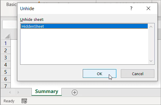
- Use a linking formula to link the data you want to show in another sheet.
For example, the following formula in the Summary sheet shows the range A1:E1 from the sheet we just made visible.
=HiddenSheet!A1:E1

- If you want, hide the sheet again by clicking on the sheet tab, then select Hide.

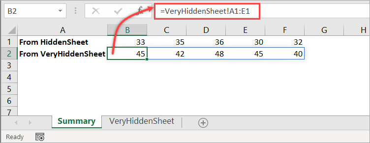
To link to a very hidden sheet in Excel
- Open the VBE by pressing Alt+F11.
- Press F4 or click View > Properties Window to open the Properties window under the Project Explorer if it’s not already open.
- In Project Explorer, select the very hidden sheet you want to unhide. Then, set its Visible property to
-1 - xlSheetVisiblein the Properties window.

- Use a linking formula to link the data you want to show in another sheet. For example, the following formula in the Summary sheet shows the range A1:E1 from the very hidden sheet we just made visible.
=VeryHiddenSheet!A1:E1
- If you want, change the sheet’s Visible property back to
2 - xlSheetVeryHiddenin the Properties window to make it a very hidden sheet again.
How to link sheets in Excel to a master sheet
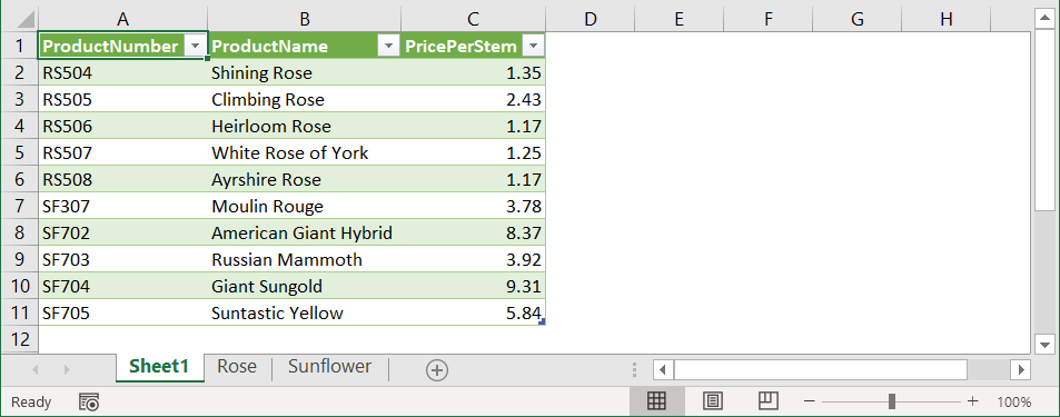
With the following spreadsheet, suppose you want to link data from two worksheets into one.

Notice that it’s like combining two ranges, which are Rose!A1:C6 and Sunflower!A1:C6.
However, combining ranges in Excel using a formula is a bit complex. An easier way to do this is using Power Query, as explained in the steps below:
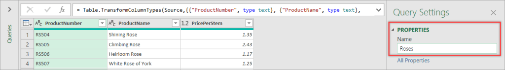
- In the Rose sheet, select the range A1:C6.
- Then, on the Data tab in the Get & Transform Data section, click From Table/Range.
- In the “Create Table” dialog box, ensure that the My table has headers option checked.

- Click OK — this will bring you to the Power Query editor.
- In the Query Settings, give your query a descriptive name, e.g., Roses.
- Click the Home tab, then click Close & Load > Close & Load To…
- In the “Import Data” dialog box, select Only Create Connection, then press OK.

- Repeat steps 1-7 for the Sunflower data. But for the fifth step, let’s rename the query as Sunflowers.
- Re-launch the Power Query editor by clicking the Data tab, then click Get Data > Launch Power Query Editor…
- Select any query, then click Append Queries > Append Queries as New to keep the existing queries unchanged.

- In the Append window, select the other table as the second table, then click OK.

- Make sure to select the newly created query. Then, on the Home tab, click Close & Load > Close & Load To…
- In the “Import Data” dialog box, load the combined data to Sheet1!A1, then click OK.
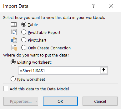
To see the result, click Sheet1. You’ll find the combined data as shown in the following screenshot:
When the source data from the other sheets change, you won’t see the new changes right away. Using this method, you need to click the Refresh All button in the Data tab to see the latest data.
How to link two Excel sheets in different workbooks
To link to a worksheet in another workbook, you can do it whether the source file is open or closed. If possible, we suggest you open all the source workbooks first before creating the links in the destination workbook. Why? Because this way is easier.
As an example, suppose you have the following four workbooks: Summary.xlsx, Jason Jones.xlsx, Melinda.xlsx, and Amanda Walker.xlsx. In the Summary workbook, you want to link the total sales of each salesperson, which is in cell F3 of each of the other workbooks—see the following screenshot:
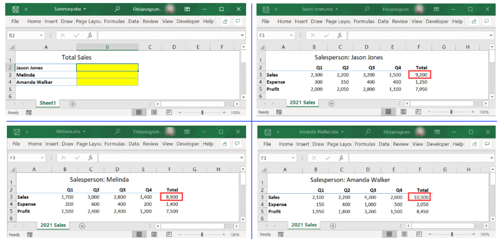
Link to another worksheet when the source workbook is open
When all the source files are open, you can follow the steps below to create the links:
- In the Summary workbook, type = (equal sign) in the destination cell for Jason Jones.

- Click View > Switch Windows, then select Jason Jones.xlsx to switch to this workbook.

- Select the cell to link, in this case, F3, then press Enter.

- Repeat Steps 1-3 for Melinda and Amanda Walker.
As the final result, you’ll see formulas with the following format when you click on each of the destination cells:
='[SourceWorkbook.xlsx]SheetName'!RangeAddress

Note: In the above example, the workbook name and/or sheet name contain spaces, so the path is enclosed in single quotation marks.
Link to another worksheet when the source workbook is closed
If you close the source workbooks one by one, the linking formulas in the Summary workbook will change as shown in the below screenshot:
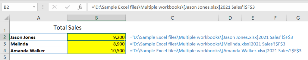
Now, you get the idea — you need to use the full path when linking to a workbook that’s currently closed.
Basically, you can use the following format to link data from any Excel workbooks:
='FolderPath[SourceWorkbook.xlsx]SheetName'!RangeAddress
However, if possible, just open the source files before you create the link, so you don’t need to manually type the long formula that’s shown above. 🙂
Can you break links between sheets in different workbooks in Excel?
When you open an Excel file, there may be formulas in it that get data from another workbook.
To locate these formulas, click on the Data tab in the ribbon. If the Edit Links button is available, it means that your file contains links to other workbooks.

To break a link, follow these steps:
- On the Data tab, in the Queries & Connections section, click Edit Links.
- In the “Edit Links” dialog box that appears, select the link you want to break and click Break Link.

- Click Break Links in the confirmation dialog box that appears.

Notice that when you break a link to the source workbook, all the linking formulas are converted to their current values. This action cannot be undone, so you may want to back up your workbook before breaking any links.
- Click Close.
In this section, you’ve learned the basics of how to link sheets from different workbooks, as well as how to break those links. If you’re interested in more examples of linking worksheets from different workbooks, check out our article on how to link Excel files.
Thanks for reading, and good luck with your data!
-

Senior analyst programmer

Back to Blog
Focus on your business
goals while we take care of your data!
Try Coupler.io
As you use and build more Excel workbooks, you’ll need to link them up. Maybe you want to write formulas that use data between different sheets in a workbook. You can even write formulas that use data from multiple different workbooks.
If I want to keep my files clean and tidy, I’ve found it’s best to separate large sheets of data from the formulas that summarize them. I often use a single workbook or sheet to summarize things.
In this tutorial, you’ll learn how to link data in Excel. First, we’ll learn how to link up data in the same workbook on different sheets. Then, we’ll move on to linking up multiple Excel workbooks to import and sync data between files.
How to Quickly Link Data in Excel Workbooks (Watch & Learn)
I’ll walk you through two examples linking up your spreadsheets. You’ll see how to pull data from another workbook in Excel and keep two workbooks connected. We’ll also walk through a basic example to write formulas between sheets in the same workbook.
Let’s walk through an illustrated guide to linking up your data between sheets and workbooks in Excel.
Basics: How to Link Between Sheets in Excel
Let’s start off by learning how to write formulas using data from another sheet. You probably already know that Excel workbooks can contain multiple worksheets. Each worksheet is a tab of its own, and you can switch tabs by clicking on them at the bottom of Excel.
Complex workbooks can easily grow to many sheets. In time, you’ll certainly need to write formulas to work with data on different tabs.
Maybe you use a single sheet in your workbook for all of your formulas to summarize your data, and separate sheets to hold the original data.
Let’s learn how to write a multi-sheet formula to work with data from multiple sheets in the same workbook.
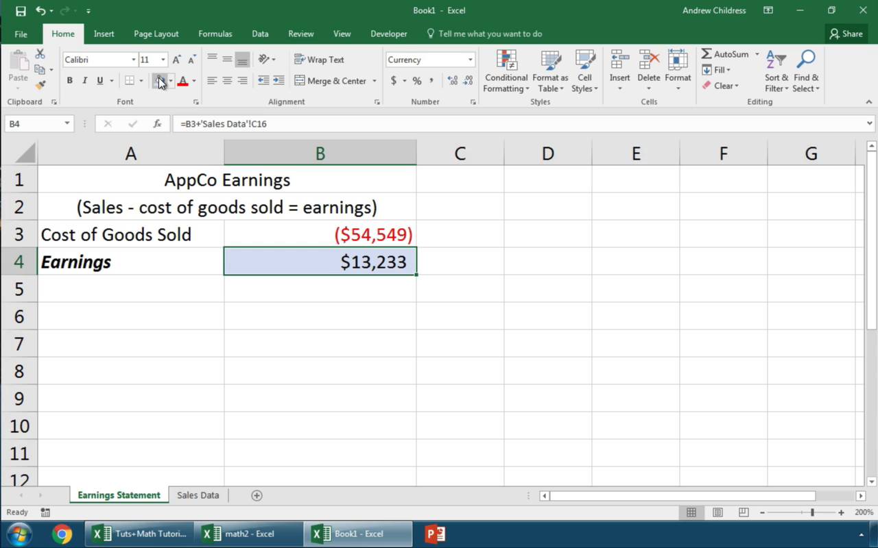
1. Start a New Formula in Excel
Most formulas in Excel start off with the equals (=) sign. Double click or start typing in a cell and begin writing the formula that you want to link up. For my example, I’ll write a sum formula to add up several cells.
I’ll open up the = sign, and then click on the first cell on my current sheet to make it the first part of the formula. Then, I’ll type a + sign to add my second cell to this formula.
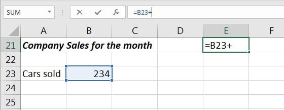

Now, make sure that you don’t close out your formula and press enter yet! You’ll want to leave the formula open before you switch sheets.
2. Switch Sheets in Excel
While you still have the formula open, click on a different sheet tab at the bottom of Excel. It’s very important that you don’t close out the formula before you click on the next cell to include as part of the formula.
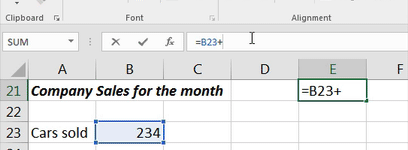

After you switch sheets, click on the next cell that you want to include in the formula. As you can see in the screenshot below, Excel automatically writes the part of the formula that references a cell on another sheet for you.
Notice in the screenshot below that to reference a cell on another sheet, Excel adds «Sheet2!B3», which simply references cell B3 on a sheet named Sheet2. You could write this manually, but clicking on the cells makes Excel write it for you automatically.

3. Finish the Excel Formula
At this point, you can press enter to close out and complete your multi-sheet formula. When you do so, Excel will jump back to where you started the formula and show you the results.
You could also keep writing the formula, including cells from more sheets and other cells on the same sheet. Keep combining those references throughout the workbook for all the data you need.
Level Up: How to Link Multiple Excel Workbooks
Let’s learn how to pull data from another workbook. With this skill, you can write formulas that pull together data from entirely separate Excel workbooks.
For this section of the tutorial, you can use two workbooks that you can download for free as a part of this tutorial. Open them both up in Excel, and follow the directions below.
1. Open Both Workbooks
Let’s start off by writing a formula that includes data from two different workbooks.
The easiest way to use this feature is to open up two Excel workbooks at the same time and put them side by side. I use the Windows Snap feature to split them to each take up half the screen. You need to keep both workbooks in view to write formulas between them.
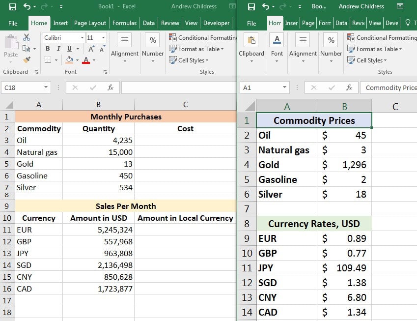
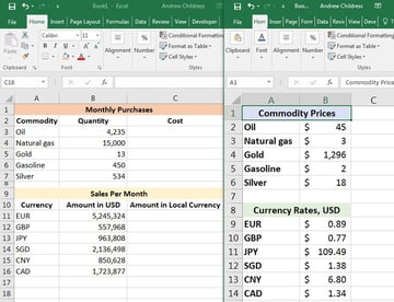
In the screenshot below, I’ve opened two workbooks that I’ll write formulas for side-by-side. For my example, I’m running a business that buys a variety of products, and sells them in a variety of countries. So, I’ll use separate workbooks to track my purchases/sales and cost data.

2. Start Writing Your Formula in Excel
The price of what I buy can change, and so can the rate that I receive payments in. I need to keep a lookup list of rates and multiply it times my purchases. This is the perfect time to link two workbooks together and write formulas between them.
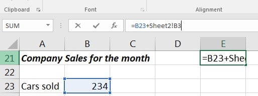
Let’s take the number of barrels of oil I buy each month times the price per barrel. In the first Cost cell (cell C3), I’ll start writing a formula by typing the equals sign (=), and then clicking on cell B3 to grab the quantity. Now, I’ll add an * to prepare to multiply the quantity by the rate.
So far, your formula should be:
=B3*


Don’t close out your formula yet. Make sure to leave it open before moving onto the next step; we still need to point Excel to the price data to multiply the quantity by.
3. Switch Excel Workbooks
It’s time to switch workbooks, and this is why it’s important to keep both of your datasets in view while working between workbooks.
With your formula still open, click over to the other workbook. Then, click on a cell in your second workbook to link up the two Excel files.


Excel automatically wrote the reference to a separate workbook as part of the cell formula:
=B3*[Prices.xlsx]Sheet1!$B$2
Once you press Enter, Excel will calculate the final cost by multiplying the quantity in the first workbook times the price in the second workbook.
Now, keep working on your Excel skills by multiplying each of the quantities or values times the reference amounts in the «Prices» workbook.
In short, the key is to get your workbooks open side by side, and simply switch workbooks to write formulas referencing other files.
There’s nothing stopping you from linking up more than two workbooks. You could open many workbooks to link up and write formulas, connecting the data between many sheets to keep cells up to date.
How to Refresh Your Data Between Workbooks
When you’ve written formulas that reference other Excel workbooks, you’ll need to think about how you’ll update your data.
So, what happens when the data changes in the workbook that you’re linking to? Will your workbook automatically update, or will you need to refresh your files to pull over the last data and import it?
The answer is, «it depends», and specifically, it depends upon if both workbooks are still open at the same time.
Example 1: Both Excel Workbooks Still Open
Let’s check out an example using the same workbook from the prior step. Both workbooks are still open. Let’s see what happens when we change the price of oil from $45 per barrel to $75 per barrel:


In the screenshot above, you can see that when we updated the price of oil, the other workbook automatically updated.
This is important to know: if both workbooks are open at the same time, changes will update automatically and in real-time. When you change one variable, the other workbook will update or recalculate based upon the new value.
Example 2: With One Workbook Closed
What if you only open one workbook at a time? For example, each morning, we update prices of our commodities and currencies, and in the evening we review the impact of the change to our purchases and sales.
The next time you open up your workbook that references other sheets, you might get a message similar to the one below. You can click on Update to pull in the latest data from your reference workbook.
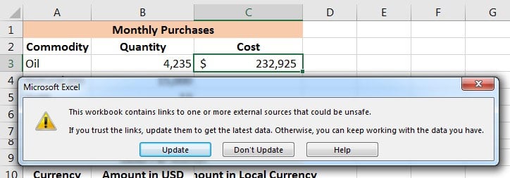


You might also see a menu where you can click Enable Content to automate updating data between Excel files.
Recap and Keep Learning More About Excel
Writing formulas between sheets and workbooks is a necessary skill when you work with Microsoft Excel. Using multiple spreadsheets inside your formulas is no problem with a bit of know-how.
Check out these additional tutorials to learn more about Excel skills and how to work with data. These tutorials are a great way to continue learning Excel.
Let me know in the comments if you have any questions about how to link up your Excel workbooks.
Did you find this post useful?

I believe that life is too short to do just one thing. In college, I studied Accounting and Finance but continue to scratch my creative itch with my work for Envato Tuts+ and other clients. By day, I enjoy my career in corporate finance, using data and analysis to make decisions.
I cover a variety of topics for Tuts+, including photo editing software like Adobe Lightroom, PowerPoint, Keynote, and more. What I enjoy most is teaching people to use software to solve everyday problems, excel in their career, and complete work efficiently. Feel free to reach out to me on my website.
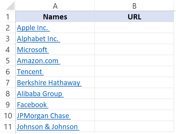
Excel allows having hyperlinks in cells which you can use to directly go to that URL.
For example, below is a list where I have company names which are hyperlinked to the company website’s URL. When you click on the cell, it will automatically open your default browser (Chrome in my case) and go to that URL.
There are many things you can do with hyperlinks in Excel (such as a link to an external website, link to another sheet/workbook, link to a folder, link to an email, etc.).
In this article, I will cover all you need to know to work with hyperlinks in Excel (including some useful tips and examples).
How to Insert Hyperlinks in Excel
There are many different ways to create hyperlinks in Excel:
- Manually type the URL (or copy paste)
- Using the HYPERLINK function
- Using the Insert Hyperlink dialog box
Let’s learn about each of these methods.
Manually Type the URL
When you manually enter a URL in a cell in Excel, or copy and paste it in the cell, Excel automatically converts it into a hyperlink.
Below are the steps that will change a simple URL into a hyperlink:
- Select a cell in which you want to get the hyperlink
- Press F2 to get into the edit mode (or double click on the cell).
- Type the URL and press enter. For example, if I type the URL – https://trumpexcel.com in a cell and hit enter, it will create a hyperlink to it.

Note that you need to add http or https for those URLs where there is no www in it. In case there is www as the prefix, it would create the hyperlink even if you don’t add the http/https.
Similarly, when you copy a URL from the web (or some other document/file) and paste it in a cell in Excel, it will automatically be hyperlinked.
Insert Using the Dialog Box
If you want the text in the cell to be something else other than the URL and want it to link to a specific URL, you can use the insert hyperlink option in Excel.
Below are the steps to enter the hyperlink in a cell using the Insert Hyperlink dialog box:
- Select the cell in which you want the hyperlink
- Enter the text that you want to be hyperlinked. In this case, I am using the text ‘Sumit’s Blog’
- Click the Insert tab.

- Click the links button. This will open the Insert Hyperlink dialog box (You can also use the keyboard shortcut – Control + K).

- In the Insert Hyperlink dialog box, enter the URL in the Address field.
- Press the OK button.
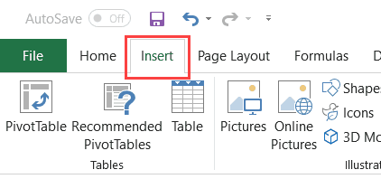


This will insert the hyperlink the cell while the text remains the same.

There are many more things you can do with the ‘Insert Hyperlink’ dialog box (such as create a hyperlink to another worksheet in the same workbook, create a link to a document/folder, create a link to an email address, etc.). These are all covered later in this tutorial.
Insert Using the HYPERLINK Function
Another way to insert a link in Excel can be by using the HYPERLINK Function.
Below is the syntax:
HYPERLINK(link_location, [friendly_name])
- link_location: This can be the URL of a web-page, a path to a folder or a file in the hard disk, place in a document (such as a specific cell or named range in an Excel worksheet or workbook).
- [friendly_name]: This is an optional argument. This is the text that you want in the cell that has the hyperlink. In case you omit this argument, it will use the link_location text string as the friendly name.
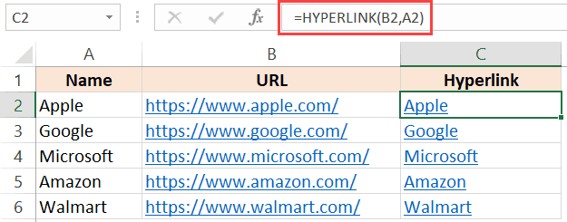
Below is an example where I have the name of companies in one column and their website URL in another column.

Below is the HYPERLINK function to get the result where the text is the company name and it links to the company website.
In the examples so far, we have seen how to create hyperlinks to websites.
But you can also create hyperlinks to worksheets in the same workbook, other workbooks, and files and folders on your hard disk.
Let’s see how it can be done.
Create a Hyperlink to a Worksheet in the Same Workbook
Below are the steps to create a hyperlink to Sheet2 in the same workbook:
- Select the cell in which you want the link
- Enter the text that you want to be hyperlinked. In this example, I have used the text ‘Link to Sheet2’.
- Click the Insert tab.
- Click the links button. This will open the Insert Hyperlink dialog box (You can also use the keyboard shortcut – Control + K).
- In the Insert Hyperlink dialog box, select ‘Place in This Document’ option in the left pane.

- Enter the cell which you want to hyperlink (I am going with the default A1).
- Select the sheet that you want to hyperlink (Sheet2 in this case)
- Click OK.
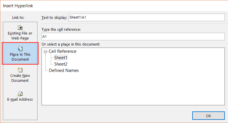

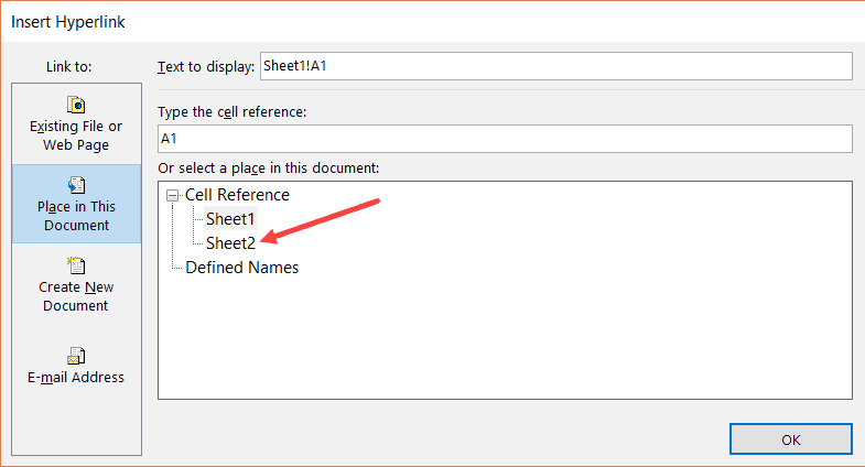
Note: You can also use the same method to create a hyperlink to any cell in the same workbook. For example, if you want to link to a far off cell (say K100), you can do that by using this cell reference in step 6 and selecting the existing sheet in step 7.
You can also use the same method to link to a defined name (named cell or named range). If you have any named ranges (named cells) in the workbook, these would be listed in under the ‘Defined Names’ category in the ‘Insert Hyperlink’ dialog box.
Apart from the dialog box, there is also a function in Excel that allows you to create hyperlinks.
So instead of using the dialog box, you can instead use the HYPERLINK formula to create a link to a cell in another worksheet.
The below formula will do this:
=HYPERLINK("#"&"Sheet2!A1","Link to Sheet2")
Below is how this formula works:
- “#” would tell the formula to refer to the same workbook.
- “Sheet2!A1” tells the formula the cell that should be linked to in the same workbook
- “Link to Sheet2” is the text that appears in the cell.
Create a Hyperlink to a File (in the same or different folders)
You can also use the same method to create hyperlinks to other Excel (and non-Excel) files that are in the same folder or are in other folders.
For example, if you want to open a file with the Test.xlsx which is in the same folder as your current file, you can use the below steps:
- Select the cell in which you want the hyperlink
- Click the Insert tab.
- Click the links button. This will open the Insert Hyperlink dialog box (You can also use the keyboard shortcut – Control + K).
- In the Insert Hyperlink dialog box, select ‘Existing File or Webpage’ option in the left pane.
- Select ‘Current folder’ in the Look in options
- Select the file for which you want to create the hyperlink. Note that you can link to any file type (Excel as well as non-Excel files)

- [Optional] Change the Text to Display name if you want to.
- Click OK.

In case you want to link to a file which is not in the same folder, you can Browse the file and then select it. To Browse the file, click on the folder icon in the Insert Hyperlink dialog box (as shown below).

You can also do this using the HYPERLINK function.
The below formula will create a hyperlink that links to a file in the same folder as the current file:
=HYPERLINK("Test.xlsx","Test File")
In case the file is not in the same folder, you can copy the address of the file and use it as the link_location.
Create a Hyperlink to a Folder
This one also follows the same methodology.
Below are the steps to create a hyperlink to a folder:
- Copy the folder address for which you want to create the hyperlink
- Select the cell in which you want the hyperlink
- Click the Insert tab.
- Click the links button. This will open the Insert Hyperlink dialog box (You can also use the keyboard shortcut – Control + K).
- In the Insert Hyperlink dialog box, paste folder address
- Click OK.

You can also use the HYPERLINK function to create a hyperlink that points to a folder.
For example, the below formula will create a hyperlink to a folder named TEST on the desktop and as soon as you click on the cell with this formula, it will open this folder.
=HYPERLINK("C:UserssumitDesktopTest","Test Folder")
To use this formula, you will have to change the address of the folder to the one you want to link to.
Create Hyperlink to an Email Address
You can also have hyperlinks which open your default email client (such as Outlook) and have the recipients email and the subject line already filled in the send field.
Below are the steps to create an email hyperlink:
- Select the cell in which you want the hyperlink
- Click the Insert tab.
- Click the links button. This will open the Insert Hyperlink dialog box (You can also use the keyboard shortcut – Control + K).
- In the insert dialog box, click on ‘E-mail Address’ in the ‘Link to’ options
- Enter the E-mail address and the Subject line

- [Optional] Enter the text you want to be displayed in the cell.
- Click OK.

Now when you click on the cell which has the hyperlink, it will open your default email client with the email and subject line pre-filled.
You can also do this using the HYPERLINK function.
The below formula will open the default email client and have one email address already pre-filled.
=HYPERLINK("mailto:abc@trumpexcel.com","Send Email")
Note that you need to use mailto: before the email address in the formula. This tells the HYPERLINK function to open the default email client and use the email address that follows.
In case you want to have the subject line as well, you can use the below formula:
=HYPERLINK("mailto:abc@trumpexcel.com,?cc=&bcc=&subject=Excel is Awesome","Generate Email")
In the above formula, I have kept the cc and bcc fields as empty, but you can also these emails if needed.
Here is a detailed guide on how to send emails using the HYPERLINK function.
Remove Hyperlinks
If you only have a few hyperlinks, you can remove these manually, but if you have a lot, you can use a VBA Macro to do this.
Manually Remove Hyperlinks
Below are the steps to remove hyperlinks manually:
- Select the data from which you want to remove hyperlinks.
- Right-click on any of the selected cell.
- Click on the ‘Remove Hyperlink’ option.


The above steps would instantly remove hyperlinks from the selected cells.
In case you want to remove hyperlinks from the entire worksheet, select all the cells and then follow the above steps.
Remove Hyperlinks Using VBA
Below is the VBA code that will remove the hyperlinks from the selected cells:
Sub RemoveAllHyperlinks()
'Code by Sumit Bansal @ trumpexcel.com
Selection.Hyperlinks.Delete
End Sub
If you want to remove all the hyperlinks in the worksheet, you can use the below code:
Sub RemoveAllHyperlinks()
'Code by Sumit Bansal @ trumpexcel.com
ActiveSheet.Hyperlinks.Delete
End Sub
Note that this code will not remove the hyperlinks created using the HYPERLINK function.
You need to add this VBA code in the regular module in the VB Editor.
If you need to remove hyperlinks quite often, you can use the above VBA codes, save it in the Personal Macro Workbook, and add it to your Quick Access Toolbar. This will allow you to remove hyperlinks with a single click and it will be available in all the workbooks on your system.
Here is a detailed guide on how to remove hyperlinks in Excel.
Prevent Excel from Creating Hyperlinks Automatically
For some people, it’s a great feature that Excel automatically converts a URL text to a hyperlink when entered in a cell.
And for some people, it’s an irritation.
If you’re in the latter category, let me show you a way to prevent Excel from automatically creating URLs into hyperlinks.
The reason this happens as there is a setting in Excel that automatically converts ‘Internet and network paths’ into hyperlinks.
Here are the steps to disable this setting in Excel:
- Click the File tab.
- Click on Options.

- In the Excel Options dialog box, click on ‘Proofing’ in the left pane.

- Click on the AutoCorrect Options button.
- In the AutoCorrect dialog box, select the ‘AutoFormat As You Type’ tab.

- Uncheck the option – ‘Internet and network paths with hyperlinks’

- Click OK.
- Close the Excel Options dialog box.


If you’ve completed the following steps, Excel would not automatically turn URLs, email address, and network paths into hyperlinks.
Note that this change is applied to the entire Excel application, and would be applied to all the workbooks that you work with.
Extract Hyperlink URLs (using VBA)
There is no function in Excel that can extract the hyperlink address from a cell.
However, this can be done using the power of VBA.
For example, suppose you have a dataset (as shown below) and you want to extract the hyperlink URL in the adjacent cell.
Let me show you two techniques to extract the hyperlinks from the text in Excel.
Extract Hyperlink in the Adjacent Column
If you want to extract all the hyperlink URLs in one go in an adjacent column, you can so that using the below code:
Sub ExtractHyperLinks()
Dim HypLnk As Hyperlink
For Each HypLnk In Selection.Hyperlinks
    HypLnk.Range.Offset(0, 1).Value = HypLnk.Address
Next HypLnk
End Sub
The above code goes through all the cells in the selection (using the FOR NEXT loop) and extracts the URLs in the adjacent cell.
In case you want to get the hyperlinks in the entire worksheet, you can use the below code:
Sub ExtractHyperLinks()
On Error Resume Next
Dim HypLnk As Hyperlink
For Each HypLnk In ActiveSheet.Hyperlinks
    HypLnk.Range.Offset(0, 1).Value = HypLnk.Address
Next HypLnk
End Sub
Note that the above codes wouldn’t work for hyperlinks created using the HYPERLINK function.
Extract Hyperlink Using a Formula (created with VBA)
The above code works well when you want to get the hyperlinks from a dataset in one go.
But if you have a list of hyperlinks that keeps expanding, you can create a User Defined Function/formula in VBA.
This will allow you to quickly use the cell as the input argument and it will return the hyperlink address in that cell.
Below is the code that will create a UDF for getting the hyperlinks:
Function GetHLink(rng As Range) As String
    If rng(1).Hyperlinks.Count <> 1 Then
        GetHLink = ""
    Else
        GetHLink = rng.Hyperlinks(1).Address
    End If
End Function
Note that this wouldn’t work with Hyperlinks created using the HYPERLINK function.
Also, in case you select a range of cells (instead of a single cell), this formula will return the hyperlink in the first cell only.
Find Hyperlinks with Specific Text
If you’re working with a huge dataset that has a lot of hyperlinks in it, it could be a challenge when you want to find the ones that have a specific text in it.
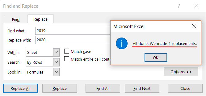
For example, suppose I have a dataset as shown below and I want to find all the cells with hyperlinks that have the text 2019 in it and change it to 2020.

And no.. doing this manually is not an option.
You can do that using a wonderful feature in Excel – Find and Replace.
With this, you can quickly find and select all the cells that have a hyperlink and then change the text 2019 with 2020.
Below are the steps to select all the cells with a hyperlink and the text 2019:
- Select the range in which you want to find the cells with hyperlinks with 2019. In case you want to find in the entire worksheet, select the entire worksheet (click on the small triangle at the top left).
- Click the Home tab.

- In the Editing group, click on Find and Select

- In the drop-down, click on Replace. This will open the Find and Replace dialog box.

- In the Find and Replace dialog box, click on the Options button.This will show more options in the dialog box.

- In the ‘Find What’ options, click on the little downward pointing arrow in the Format button (as shown below).

- Click on the ‘Choose Format From Cell’. This will turn your cursor into a plus icon with a format picker icon.

- Select any cell which has a hyperlink in it. You will notice that the Format gets visible in the box on the left of the Format button. This indicates that the format of the cell you selected has been picked up.
- Enter 2019 in the ‘Find What’ field and 2020 in the ‘Replace with’ field.
- Click on the Replace All button.


In the above data, it will change the text of four cells that have the text 2019 in it and also has a hyperlink.
You can also use this technique to find all the cells with hyperlinks and get a list of it. To do this, instead of clicking on Replace All, click on the Find All button. This will instantly give you a list of all the cell address that has hyperlinks (or hyperlinks with specific text depending on what you’ve searched for).
Note: This technique works as Excel is able to identify the formatting of the cell that you select and use that as a criterion to find cells. So if you’re finding hyperlinks, make sure you select a cell that has the same kind of formatting. If you select a cell that has a background color or any text formatting, it may not find all the correct cells.
Selecting a Cell that has a Hyperlink in Excel
While Hyperlinks are useful, there are a few things about it that irritate me.
For example, if you want to select a cell that has a hyperlink in it, Excel would automatically open your default web browser and try to open this URL.
Another irritating thing about it is that sometimes when you have a cell that has a hyperlink in it, it makes the entire cell clickable. So even if you’re clicking on the hyperlinked text directly, it still opens the browser and the URL of the text.
So let me quickly show you how to get rid of these minor irritants.
Select the Cell (without opening the URL)
This is a simple trick.
When you hover the cursor over a cell that has a hyperlink in it, you’ll notice the hand icon (which indicates if you click on it, Excel will open the URL in a browser)
![]()
Click the cell anyway and hold the left button of the mouse.
After a second, you’ll notice that the hand cursor icon changes into the plus icon, and now when you leave it, Excel will not open the URL.
![]()
Instead, it would select the cell.
Now, you can make any changes in the cell you want.
Neat trick… right?
Select a Cell by clicking on the blank space in the cell
This is another thing that might drive you nuts.
When there is a cell with the hyperlink in it as well as some blank space, and you click on the blank space, it still opens the hyperlink.
![]()
Here is a quick fix.
This happens when these cells have the wrap text enabled.
If you disable wrap text for these cells, you will be able to click on the white space on the right of the hyperlink without opening this link.
Some Practical Example of Using Hyperlink
There are useful things you can do when working with hyperlinks in Excel.
In this section, I am going to cover some examples that you may find useful and can use in your day-to-day work.
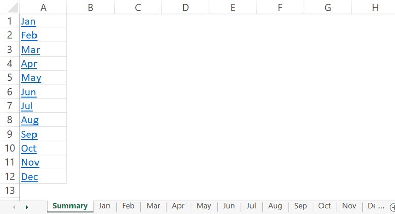
Example 1 – Create an Index of All Sheets in the Workbook
If you have a workbook with a lot of sheets, you can use a VBA code to quickly create a list of the worksheets and hyperlink these to the sheets.
This could be useful when you have 12-month data in 12 different worksheets and want to create one index sheet that links to all these monthly data worksheets.
Below is the code that will do this:
Sub CreateSummary()
'Created by Sumit Bansal of trumpexcel.com
'This code can be used to create summary worksheet with hyperlinks
Dim x As Worksheet
Dim Counter As Integer
Counter = 0
For Each x In Worksheets
Counter = Counter + 1
If Counter = 1 Then GoTo Donothing
    With ActiveCell
        .Value = x.Name
        .Hyperlinks.Add ActiveCell, "", x.Name & "!A1", TextToDisplay:=x.Name, ScreenTip:="Click here to go to the Worksheet"
        With Worksheets(Counter)
            .Range("A1").Value = "Back to " & ActiveSheet.Name
            .Hyperlinks.Add Sheets(x.Name).Range("A1"), "", _
            "'" & ActiveSheet.Name & "'" & "!" & ActiveCell.Address, _
            ScreenTip:="Return to " & ActiveSheet.Name
        End With
    End With
ActiveCell.Offset(1, 0).Select
Donothing:
Next x
End Sub
You can place this code in the regular module in the workbook (in VB Editor)
This code also adds a link to the summary sheet in cell A1 of all the worksheets. In case you don’t want that, you can remove that part from the code.
You can read more about this example here.
Note: This code works when you have the sheet (in which you want the summary of all the worksheets with links) at the beginning. In case it’s not at the beginning, this may not give the right results).
Example 2 – Create Dynamic Hyperlinks
In most cases, when you click on a hyperlink in a cell in Excel, it will take you to a URL or to a cell, file or folder. Normally, these are static URLs which means that a hyperlink will take you to a specific predefined URL/location only.
But you can also use a little bit for Excel formula trickery to create dynamic hyperlinks.
By dynamic hyperlinks, I mean links that are dependent on a user selection and change accordingly.
For example, in the below example, I want the hyperlink in cell E2 to point to the company website based on the drop-down list selected by the user (in cell D2).

This can be done using the below formula in cell E2:
=HYPERLINK(VLOOKUP(D2,$A$2:$B$6,2,0), "Click here")
The above formula uses the VLOOKUP function to fetch the URL from the table on the left. The HYPERLINK function then uses this URL to create a hyperlink in the cell with the text – ‘Click here’.
When you change the selection using the drop-down list, the VLOOKUP result will change and would accordingly link to the selected company’s website.
This could be a useful technique when you’re creating a dashboard in Excel. You can make the hyperlinks dynamic depending on the user selection (which could be a drop-down list or a checkbox or a radio button).
Here is a more detailed article of using Dynamic Hyperlinks in Excel.
Example 3 – Quickly Generate Simple Emails Using Hyperlink Function
As I mentioned in this article earlier, you can use the HYPERLINK function to quickly create simple emails (with pre-filled recipient’s emails and the subject line).
Single Recipient Email Id
=HYPERLINK("mailto:abc@trumpexcel.com","Generate Email")
This would open your default email client with the email id abc@trumpexcel.com in the ‘To’ field.
Multiple Recipients Email Id
=HYPERLINK("mailto:abc@trumpexcel.com,def@trumpexcel.com","Generate Email")
For sending the email to multiple recipients, use a comma to separate email ids. This would open the default email client with all the email ids in the ‘To’ field.
Add Recipients in CC and BCC List
=HYPERLINK("mailto:abc@trumpexcel.com,def@trumpexcel.com?cc=123@trumpexcel.com&bcc=456@trumpexcel.com","Generate Email")
To add recipients to CC and BCC list, use question mark ‘?’ when ‘mailto’ argument ends, and join CC and BCC with ‘&’. When you click on the link in excel, it would have the first 2 ids in ‘To’ field, 123@trumpexcel.com in ‘CC’ field and 456@trumpexcel.com in the ‘BCC’ field.
Add Subject Line
=HYPERLINK("mailto:abc@trumpexcel.com,def@trumpexcel.com?cc=123@trumpexcel.com&bcc=456@trumpexcel.com&subject=Excel is Awesome","Generate Email")
You can add a subject line by using the &Subject code. In this case, this would add ‘Excel is Awesome’ in the ‘Subject’ field.
Add Single Line Message in Body
=HYPERLINK("mailto:abc@trumpexcel.com,def@trumpexcel.com?cc=123@trumpexcel.com&bcc=456@trumpexcel.com&subject=Excel is Awesome&body=I love Excel","Email Trump Excel")
This would add a single line ‘I love Excel’ to the email message body.
Add Multiple Lines Message in Body
=HYPERLINK("mailto:abc@trumpexcel.com,def@trumpexcel.com?cc=123@trumpexcel.com&bcc=456@trumpexcel.com&subject=Excel is Awesome&body=I love Excel.%0AExcel is Awesome","Generate Email")
To add multiple lines in the body you need to separate each line with %0A. If you wish to introduce two line breaks, add %0A twice, and so on.
Here is a detailed article on how to send emails from Excel.
Hope you found this article useful.
Let me know your thoughts in the comments section.
You May Also Like the Following Excel Tutorials:
- Excel AutoCorrect
- How to Find External Links and References in Excel
- 100+ Excel Interview Questions & Answers
- Excel Text to Columns
- Excel Sparklines