
-
Create a table
Video
-
Sort data in a table
Video
-
Filter data in a range or table
Video
-
Add a Total row to a table
Video
-
Use slicers to filter data
Video
Sign in with Microsoft
Sign in or create an account.
Hello,
Select a different account.
You have multiple accounts
Choose the account you want to sign in with.
Thank you for your feedback!
×
By turning an Excel range into a table, you can work with the table data independently from the rest of the worksheet, and filter buttons appear automatically on the column headers, allowing you to filter and sort columns even faster. You can also add total rows and quickly apply table formatting.
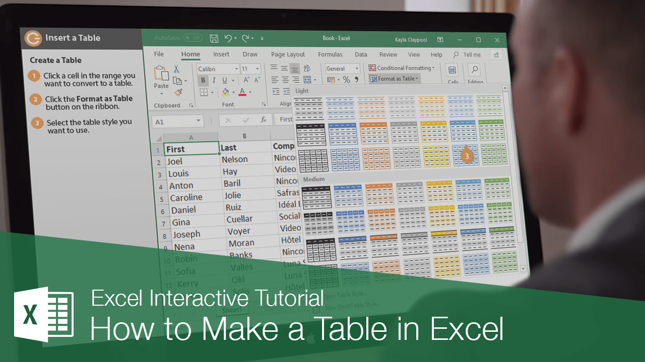
Create a Table
If you already have an organized range of data, you can turn it into a table. Before turning a range of data into a table, remove blank rows and columns, and make sure that a single column doesn’t have different types of data within it.
- Click a cell in the range you want to convert to a table.
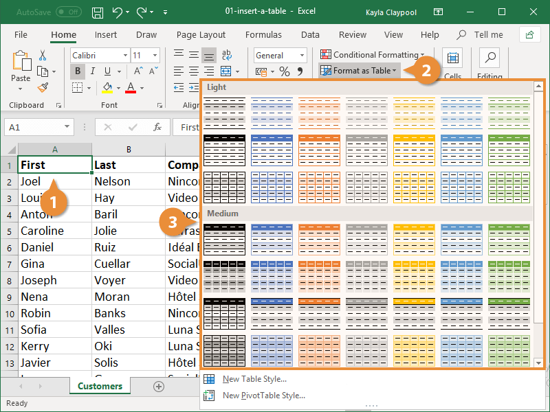
- Click the Format as Table button on the Home tab.
- Select the table style you want to use.

You can also click the Insert tab on the Ribbon and click the Table button in the Tables group.
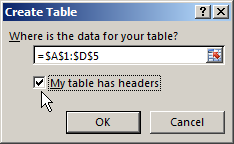
- Verify the data range includes all the cells you want to include in the table.
Make sure to specify whether the table has a header row. If it doesn’t, Excel will add a header row above the table data.
- Click OK.
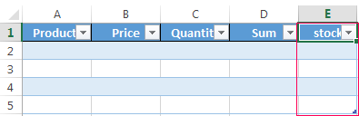
The table is created. Filters are added to each column and the table is automatically formatted. Under Table Tools on the Ribbon, the Design tab appears.
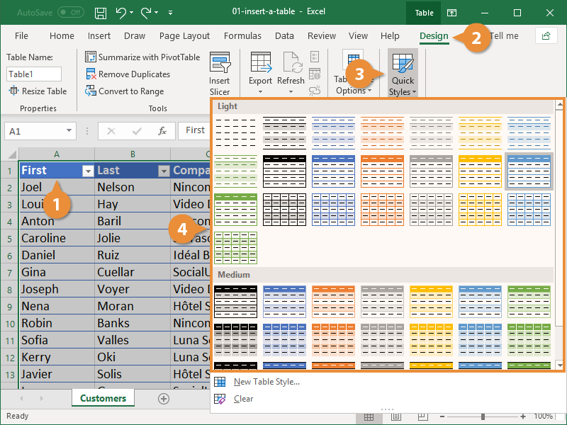
Apply a Table Style
You can change the appearance of a table at any time by applying a preset table formatting style.
- Click a cell in the table.
- Click the Design tab.
- Click the Quick Styles button from the Table Style group.
The table styles gallery appears. Here you can select styles from the Light, Medium, or Dark categories. You may need to scroll down the list to see the Dark category.
- Select a style.
Convert to a Range
If a table is no longer needed, turn it back into a normal range of data.
- Click a cell in the table.
- Click the Design tab.
- Click the Convert to Range button.
- Click Yes.
Right-click a cell in the table and select Table, then Convert to Range from the contextual menu.
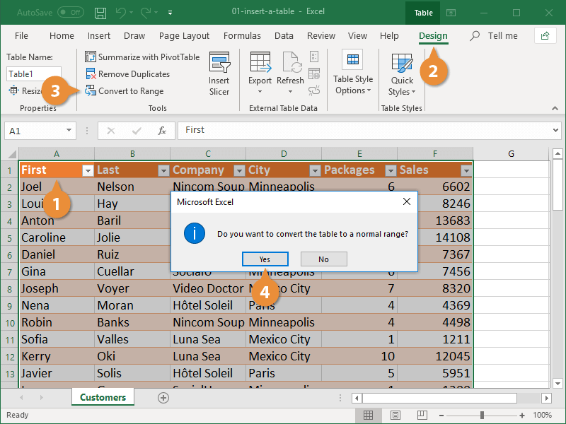
The table converts back to a normal range of cells, but the table formatting is still applied.
If you don’t want the table formatting to be applied, click the Quick Styles button on the Design tab and select None before converting the table to a range.

FREE Quick Reference
Click to Download
Free to distribute with our compliments; we hope you will consider our paid training.
Microsoft Excel is convenient for creating tables and doing calculations. Its working area is a set of cells to be filled with data. Consequently, the data can be formatted, used for building graphs, charts, summary reports.
For a beginner, working with tables in Excel may seem complicated at the first glance. It is differs considerably from the principles of table construction in Word. However, let us start from the very basics: creating and formatting tables. By the time you reach the end of this article, you will understand there is no better tool for creating tables than Excel.
Creating a table in Excel: a dummy’s guide
Working with Excel tables for dummies does not tolerate haste. There are different ways to create a table for a specific purpose, and each of them has its advantages. Therefore, let us start with assessing the situation visually.
Look carefully at the work sheet of the table processor:
It is a set of cells in columns and rows. Essentially, it’s a table. The columns are marked with letters. The rows are designated with numbers. There are no borders.
First of all, let’s learn to work with cells, rows and columns.
How to select a column and a row
To select the entire column, left-click on the letter that marks it.
To select a row, click on the number it’s designated with.
To select several columns or rows, left-click on the name, hold down the button and drag the pointer.
To select a column with the help of hot keys, place the cursor in any cell of the column and press Ctrl + Space. The key combination Shift + Space is used to select a row.
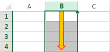
How to resize cells
If your information does not fit in the table, you need to resize the cells.
- You can move them manually by grabbing the cell boundary with the left mouse button.
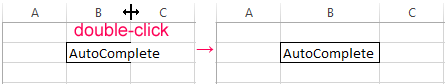
- If the cell contains a long word, you can double-click on the boundary of the column/row. The program will expand its boundary automatically.
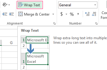
- If you need to increase the height of a row preserving the column width, use the button «Wrap Text» in the tool bar.
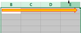
To change the column width and the row height in a certain range, resize 1 column/row (by dragging its boundaries manually) – and all the selected columns and rows will be resized automatically.
Important note. To go back to the previous size, you can press the «Undo Typing» button or the hot-key combination CTRL+Z. However, it works only if used immediately. Later on, it will not help.
To bring the rows to their initial boundaries, open the tool menu: «HOME»-«Format» and choose «AutoFit Row Height».
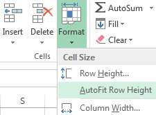
This method does not work for columns. Click «Format» — « AutoFit Row Width» Memorize this number. Select any cell in the column that needs to go back to the initial size. Click «Format» — «Column Width» again and enter the value suggested by the program (as a rule, it’s 8.43 – the number of characters in the Calibri font, size 11 pt). OK.
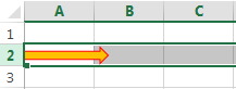
How to insert a column or row
Select the column/row to the right of/below the place where the insertion needs to be made. That is, the new column will appear to the left of the selected cell. The new row will be pasted above it.
Right-click on the cell and select «Insert» in the drop-down menu (or hit the hot-key combination CTRL+SHIFT+»=»).
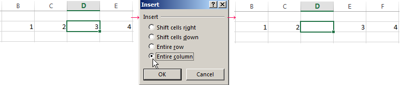
Select «Entire column» and press OK.
Hint. To insert a new column quickly, select a column in the desired position and hit CTRL+SHIFT+PLUS.
All these skills will come handy when building a table in Excel. You will need to resize the cells and insert rows/columns in the process.
Creating a table with formulas step by step
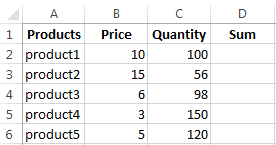
- Fill in the header manually by entering the column headings. Fill in the rows by entering your data. Apply the acquired knowledge in practice: expand the column boundaries, adjust the row height.
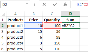
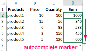
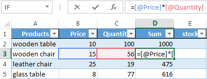
- To fill in the «Sum» column, place the cursor in its first cell. Enter «=». In such a way, we inform Excel: a formula will be here. Select the cell B2 (with the first price). Enter the multiplication symbol (*). Select the cell C2 (with the quantity). Press ENTER.
- When you hover the pointer over the cell containing the formula, a small cross will appear in its bottom right corner. It points out the autocomplete marker. Grab it with the left mouse button and drag it to the end of the column. The formula will be copied into every cell.
- Designate the boundaries of your table. Select the range containing your data. Click the button «HOME»-«Border» (on the main page in the «Font» menu). And click «All Borders».
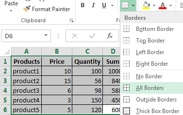
Now the column and row borders will be visible when you print the table.
The «Font» menu allows you to format the data in your Excel table the way you would do it in Word.
For example, change the font size and highlight the header in bold. You may also apply center alignment, word wrap, etc.
Creating a table in Excel: a step-by-step instruction
You already know the simplest way to create tables. However, Excel can offer a more convenient variant (in terms of the subsequent formatting and work with the data).
Let us construct a smart (dynamic) table:
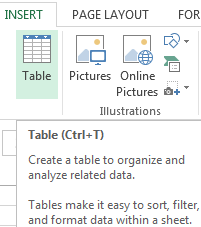
- Go to the «INSERT» tab – the «Table» tool (or press the hot-key combination CTRL+T).
- This will open a dialog window, in which you need to enter the data range. Check the box for a table with headings. Click OK. It’s no big deal if you don’t enter the proper range on the first try. The smart table is flexible, dynamic.
Important note. You can also take an alternative route: start with selecting the range of cells, then press the «Table» button.
Now enter your data into the ready framework. If you need an additional column, place the cursor in the heading cell. Make the entry and press ENTER. The range will expand automatically.

If you need additional rows, grab the autocomplete marker in the bottom right corner and drag it downward.
How to work with a table in Excel
With the release of new versions of the program, working with tables in Excel has become more interesting and dynamic. After a smart table has been formed on the spreadsheet, the tool «TABLE TOOLS» — «DESIGN» becomes available.
Here you can name the table or resize it.
Various styles are available to you, as well as the opportunity to transform the table into a regular range or a consolidated sheet.
MS Excel dynamic electronic tables offer immense opportunities. Let us begin with the basic skills of data entry and autocompletion:
- Select a cell by clicking on it with the left mouse button. Enter the text/numeric value. Press ENTER. If you need to change the value, place the cursor in the cell again and enter the new data.
- When you enter a value repetitively, Excel will recognize it. You will only need to enter several symbols and press enter.
- In a smart table, to apply a formula to the entire column, enter it in the first cell. The program will copy the formula in other cells automatically.
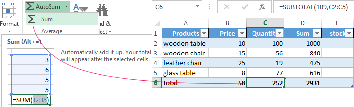
- To calculate the totals, select the column containing the values plus an empty cell for the future total and click the «Sum» button (the «Editing» tool group on the «HOME» tab, or press the hot-key combination ALT+»=»).
When you click on the little arrow to the right of every subheading in the header, you obtain access to the additional tools for working with the data in the table.
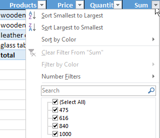
Sometimes the user has to work with huge tables, in which you need to scroll several thousand rows to see the totals. Deleting the rows is not an option (you will still need the data later). However, you can hide them. To this end, use number filters (depicted in the image above). Uncheck the values that need to be hidden.
![]()
Download Article
![]()
Download Article
This wikiHow teaches you how to create a table of information in Microsoft Excel. You can do this on both Windows and Mac versions of Excel.
-

1
Open your Excel document. Double-click the Excel document, or double-click the Excel icon and then select the document’s name from the home page.
- You can also open a new Excel document by clicking Blank Workbook on the Excel home page, but you’ll need to input your data before continuing.
-
2
Select your table’s data. Click the cell in the top-left corner of the data group you want to include in your table, then hold down ⇧ Shift while clicking the bottom-right cell in the data group.
- For example: if you have data in cells A1 down to A5 and over to D5, you would click A1 and then click D5 while holding ⇧ Shift.
Advertisement
-
3
Click the Insert tab. It’s a tab in the green ribbon at the top of the Excel window. Doing so will display the Insert toolbar below the green ribbon.
- If you’re on a Mac, make sure you don’t click the Insert menu item in your Mac’s menu bar.
-
4
Click Table. This option is in the «Tables» section of the toolbar. Clicking it brings up a pop-up window.
-
5
Click OK. It’s at the bottom of the pop-up window. Doing so will create your table.
- If your data group has cells at the top of it that are dedicated to column names (e.g., headers), click the «My table has headers» checkbox before you click OK.


Advertisement
-
1
Click the Design tab. It’s in the green ribbon near the top of the Excel window. This will open a toolbar for your table’s design directly below the green ribbon.
- If you don’t see this tab, click your table to prompt it to appear.
-
2
Select a design scheme. Click one of the colored boxes in the «Table Styles» section of the Design toolbar to apply the color and design to your table.
- You can click the downward-facing arrow to the right of the colored boxes to scroll through different design options.
-
3
Review the other design options. In the «Table Style Options» section of the toolbar, check or uncheck any of the following boxes:
- Header Row — Checking this box places column names in the top cell of the data group. Uncheck this box to remove headers.
- Total Row — When enabled, this option adds a row at the bottom of the table that displays the total value of the right-most column.
- Banded Rows — Check this box to color in alternating rows, or uncheck it to leave all rows in your table the same color.
- First Column and Last Column — When enabled, these options make the headers and data in the first and/or last columns bold.
- Banded Columns — Check this box to color in alternating columns, or uncheck it to leave all columns in your table the same color.
- Filter Button — When checked, this box places a drop-down box next to each header in your table that allows you to change the data displayed in that column.
-
4
Click the Home tab again. This will take you back to the Home toolbar. Your table’s changes will remain.


Advertisement
-
1
Open the filter menu. Click the drop-down arrow to the right of the header for the column whose data you want to filter. A drop-down menu will appear.
- In order to do this, you must have both the «Header Row» and the «Filter» boxes checked in the «Table Style Options» section of the Design tab.
-
2
Select a filter. Click one of the following options in the drop-down menu:
- Sort Smallest to Largest
- Sort Largest to Smallest
- You may also have additional options such as Sort by Color or Number Filters depending on your data. If so, you can select one of these options and then click a filter in the pop-out menu.
-
3
Click OK if prompted. Depending on the filter you choose, you may also have to select a range or a different type of data before you can continue. Your filter will be applied to your table.


Advertisement
Add New Question
-
Question
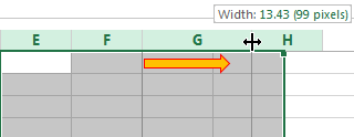
How do I resize the columns?

Place your mouse between the columns until the cursor changes into a double arrow pointing to the left and to the right. Left click and hold. Drag the mouse, while holding the left button, to the left to shrink or to the right to enlarge the column.
-
Question
How do I change the width of a column in Excel?
If you go up to «Format,» and select «Width» you will be able to change the size.
-
Question
How do I make a table in Excel fit the size of a paper?
In Excel 2013, click the «Page Layout» tab, then click the «Size» dropdown menu. Most printers use 8.5 x 11 inch paper.
See more answers
Ask a Question
200 characters left
Include your email address to get a message when this question is answered.
Submit
Advertisement
Video
-
If you no longer need the table, you can either delete it entirely or turn it back into a range of data on the spreadsheet page. To delete the table entirely, select the table and press your keyboard «Delete» key. To change it back to a range of data, right-click any of its cells, select «Table» from the popup menu that appears, and then select «Convert to Range» from the Table submenu. The sort and filter arrows disappear from the column headers, and any table name references in the cell formulas are removed. The column header names and the table formatting remain, however.
-
If you place your table so that the header for the first column is in the upper left corner of the spreadsheet (Cell A1), the column headers will replace the spreadsheet’s column headers when you scroll up. If you place the table anywhere else, the column headers will scroll out of view when you scroll up, and you’ll need to use Freeze Panes to keep them constantly displayed.
Thanks for submitting a tip for review!
Advertisement
About This Article
Article SummaryX
1. Open a file with data.
2. Select data for the table.
3. Click Insert.
4. Click Table.
5. Click OK.
Did this summary help you?
Thanks to all authors for creating a page that has been read 553,274 times.