
Содержание
- How to Graph an Equation / Function – Excel & Google Sheets
- How to Graph an Equation / Function in Excel
- Set up your Table
- Fill in Y Column
- Creating Scatterplot
- Add Equation Formula to Graph
- Final Scatterplot with Equation
- How to Graph an Equation / Function in Google Sheets
- Creating a Scatterplot
- Adding Equation
- Final Scatterplot with Equation
- Business Calculus with Excel
- Section 1.4 Graphing functions with Excel
- Example 1.4.1 . A basic graph.
- Example 1.4.3 . A graph with parameters.
- Example 1.4.5 . Controlling the viewing window.
- Example 1.4.7 . Graphing more than one function.
- Formatting a chart.
- Online graphing tools: Wolfram Alpha.
- Exercises Exercises 1.4 Graphing functions with Excel
How to Graph an Equation / Function – Excel & Google Sheets
This tutorial will demonstrate how to graph a Function in Excel & Google Sheets.
How to Graph an Equation / Function in Excel
Set up your Table
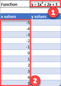
- Create the Function that you want to graph
- Under the X Column, create a range. In this example, we’re range from -5 to 5
Fill in Y Column
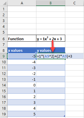
Create a formula using the Function, substituting x with what is in Column B.
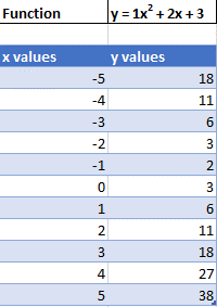
After using this formula for all the rows, you should have a table that looks like below.
Creating Scatterplot
- Highlight Dataset
- Select Insert
- Select Scatterplot
- Select Scatter with Smooth Lines
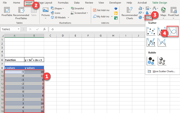
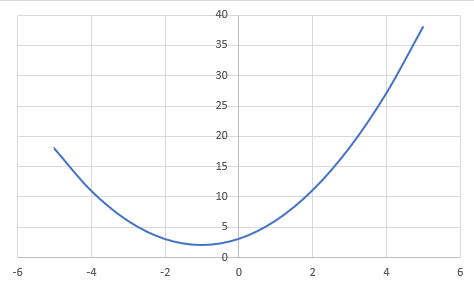
This will create a graph that should look similar to below.
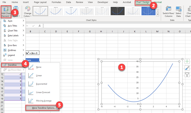
Add Equation Formula to Graph
- Click Graph
- Select Chart Design
- Click Add Chart Element
- Click Trendline
- Select More Trendline Options
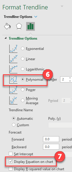
6. Select Polynomial
7. Check Display Equation on Chart
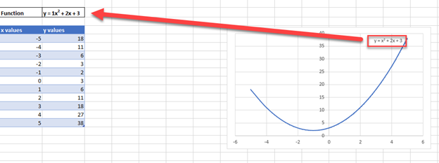
Final Scatterplot with Equation
Your final equation on the graph should match the function that you began with.
How to Graph an Equation / Function in Google Sheets
Creating a Scatterplot
- Using the same table that we made as explained above, highlight the table
- Click Insert
- Select Chart
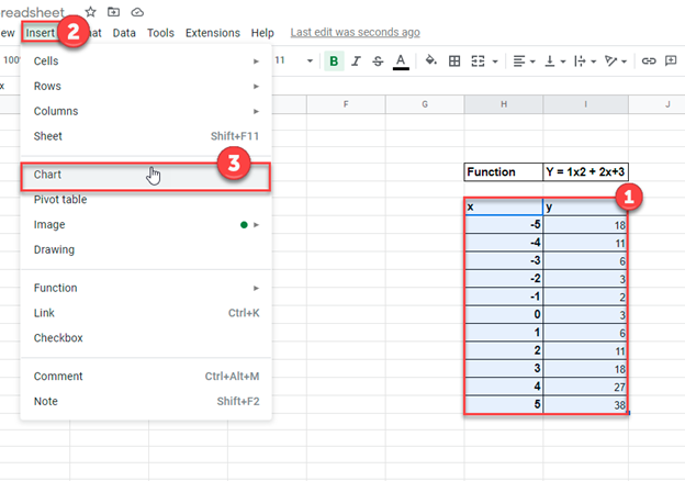
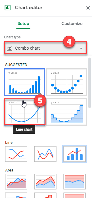
4. Click on the dropdown under Chart Type
5. Select Line Chart
Adding Equation
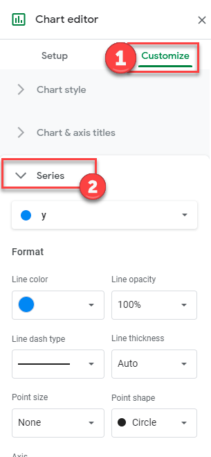
- Click on Customize
- Select Series
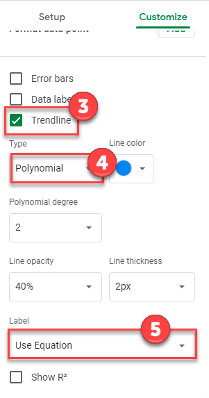
3. Check Trendline
4. Under Type, Select Polynomial
5. Under Label, Select Use Equation
Final Scatterplot with Equation
As you can see, similar to the exercise in Excel, the equation matches the function that we began with.
Источник
Business Calculus with Excel
Mike May, S.J., Anneke Bart
Section 1.4 Graphing functions with Excel
One area where Excel is different from a graphing calculator is in producing the graph of a function that has been defined by a formula. It is not difficult, but it is not as straight forward as with a calculator. It is a skill worth developing however. When we are given a formula as part of a problem, we will want to easily see a graph of the function.
We will walk through the process for producing graphs for three examples of increasing complexity. For the first example we have a specific function and specific range in mind, say (y=x^2-6 x) over (-10 le x le 10text<.>) For the second example, we would like to use parameters in the formula, for example, (y = a x^2 + b x + ctext<,>) with specified values of a, b, and c, and have the ability to easily change the values of the parameters and see the graph. For the third example we would also like to have the ability to change the domain, graphing over (xLow le x le xHightext<,>) where (xLow) and (xHigh) can easily be changed.
Example 1.4.1 . A basic graph.
Graphing (y=x^2-6 x) over (-10 le x le 10)
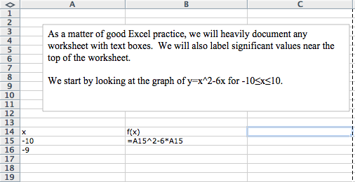
We start by producing a column for (x) and one for (f(x)text<.>) In the column for (x) we start with values (-10) and (-9text<,>) so that we can complete the column with a quick fill. Similarly, we start the (f(x)) columns in the first cell with the “ (x) ” replaced by the appropriate cell reference. In this case the formula for (f(x)) is in cell B15 and (x) is in cell A15 .
We then use quick fill and quick copy to fill out the table.
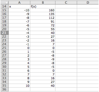
With the values of the cells filled in we highlight the cells we want to graph ( A14 through B35 ) and add a scatter plot for the highlighted values.
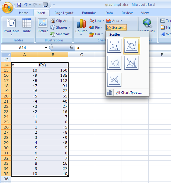
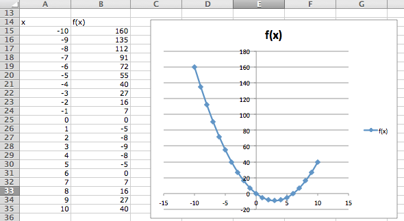
(The location of the scatterplot will be a bit different with Macs. The scatterplot is in the Charts ribbon, under other, on Macs.) This gives the desired graph.
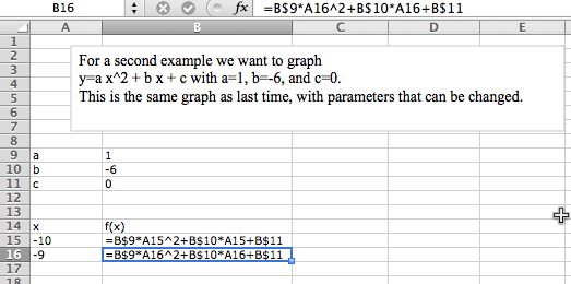
Example 1.4.3 . A graph with parameters.
Graphing (y=x^2-6 x) as an example of (y = a x^2 + b x + c) over the domain (-10 le x le 10text<.>)
For the second example, we want the same graph, but we want the ability to easily convert the graph of our first quadratic into a different quadratic function. The solution is to consider (atext<,>) (btext<,>) and (c) to be parameters that we can change.
Toward the top of the worksheet, we put the labels (atext<,>) (btext<,>) and (ctext<,>) and give values for those parameters. In this case the values of (atext<,>) (btext<,>) and (c) are in cells B9 , B10 , and B11 respectively.
Now we set up the problem in the same way we did above except that we are using absolute references for (atext<,>) (btext<,>) and (ctext<,>) and relative references for (xtext<.>)
Now, we once again do a quick fill to complete the table, and then add a scatterplot.
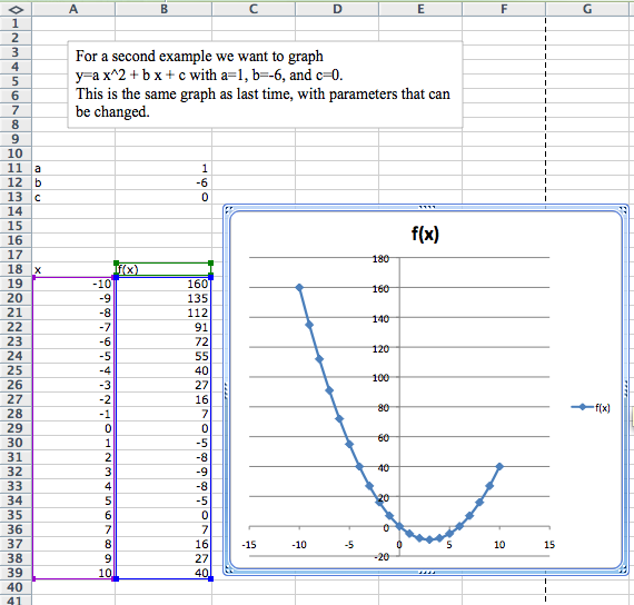
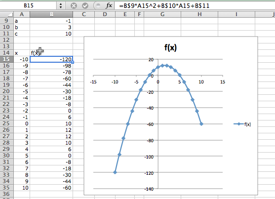
The difference with this second example is that if I now want to look at the graph of (y = -x^2 + 3 x + 10text<,>) I simply change the values of the parameters (atext<,>) (btext<,>) and (ctext<.>)
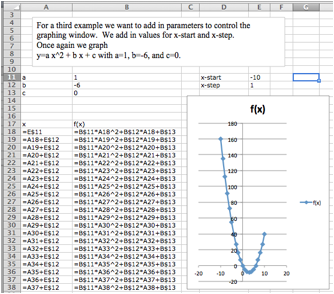
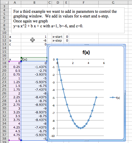
Example 1.4.5 . Controlling the viewing window.
Graphing (y=x^2 — 6 x) as an example of (y = a x^2 + b x + c) over the domain (-10 le x le 10text<,>) but with the ability to easily change the domain of the graph.
Often, when we graph, we will want to change the domain of the graph. Most easily, I may want to zoom in on a particular region to get a better view of some interesting feature. I may want to look closely at several different regions.
To do this we will again plot 21 points, but we want to have control of the starting point and the change in x between the first and second points. First we add labels and values for x-start and x-step . Then we need a bit of care in defining the values of (xtext<.>) The first value of (x) (cell A18 ) is the value of x-start . Every other value of x is defined as the previous value of x plus the value of x-step .
In this case I want a better look at the vertex of the parabola. I decide I want to see the graph for (0 le x le 5text<.>) My value for x-start is 0. My value for x-step is one twentieth of the distance from 0 to 5, or ((5-0)/20 = 0.25text<.>) I plug those values in and see the graph.
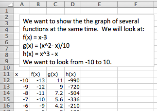
Example 1.4.7 . Graphing more than one function.
We would also like to put two or more graphs together. For our examples, we will want to use the functions (f(x) = x — 3text<,>) (g(x) = (x^2 — x)/10text<,>) and (h(x) = x^3 — xtext<.>) We start by using the procedure given above to make a chart of values for the three functions.
We then simply select the cells for (x) and the functions we want graphed together and produce a scatterplot as before. (To graph (g(x)) and (h(x)) together, we want to select the columns for (xtext<,>) (g(x)text<,>) and (h(x)text<.>) )
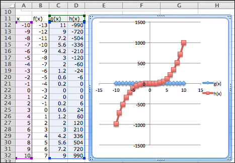
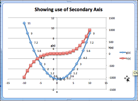
One problem with the graph of (g(x)) and (h(x)) together is that the functions have different orders of magnitude, so we do not see that (y = g(x)) is a parabola. One remedy is to use a secondary axis for the graph of (h(x)text<.>) (Simply double click on one of the points for (h(x)text<,>) and select secondary axis from the axes tab.)

Formatting a chart.
Excel has a lot of ways to add formatting to a graph or chart, many more than we want to be concerned with at this point. We simply point out a few and leave it to the reader to explore how this should be used for a good visual presentation. If you click once on the chart to select it, the Chart tab in the home ribbon, adds sub-tabs for layout and format. With Chart Title, you can add a title to the chart, then edit it. The Axes icon allows you to add titles for the axes. If you select a data point form (g(x)text<,>) you can then use the Data Labels icon to add values next to the points. The chart with these annotations is given below. The rule of thumb to follow is to add enough annotations for a reader to be able to easily understand what is happening in the chart.
It is also worthwhile to note that you can manually set the y-range of a graph by double clicking on the axis and setting the values. This is particularly useful of the function has a vertical asymptote.
Online graphing tools: Wolfram Alpha.
Throughout this book, we are limiting ourselves to mathematical tools that the student can reasonably expect to find in a generic work environment. That is one of the reasons for focusing on using spreadsheets and Excel. A second reason is that we will spend a significant amount of time on functions defined by data points, where we then try to construct a formula. However when we are starting with a formula, there are easier ways to produce a graph. The simplest is to use the free website, Wolfram Alpha  3  . For example to obtain a graph of the functions (f(x) = x^2 — 3 xtext<,>) as (x) ranges from (-5) to (5text<,>) we simply type “ plot x^2 — 3 x for x from -5 to 5 ” and obtain:

We will return to Wolfram Alpha from time to time, when we have nice formulas to manipulate.
Exercises Exercises 1.4 Graphing functions with Excel
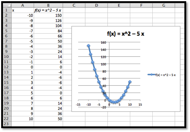
Produce a worksheet that with a graph of the function (f(x) = x^2 — 5 xtext<,>) with (x) going from -10 to 10 by 1.
The entry in cell B2 is =A2^2-5*A2 ; remember to use quickfill to complete the table
Produce a worksheet that with a graph of the function (g(x) = (x^2 — 5 x)/(x^2 + 7 x + 10)text<,>) with (x) going from -10 to 10 by 1. Explain why the graph is inaccurate. (Pay attention to places where there should be asymptotes.)
2* – Extra credit) — Fix the graph from problem 2 by adjusting the set of (x) -values used.
Produce a worksheet with a graph of (h(x) = x^3 + a x^2 + b x + c) for (x) from -10 to 10, where the values of (atext<,>) (btext<,>) and (c) can be changed and the graph will update automatically. For initial values, use (a = -2text<,>) (b = 1text<,>) and (c = -11text<.>)
The entry in B5 should be =A5^3+$B$1*A5^2+$B$2*A5+$B$3 . Note that the references to (atext<,>) (b) and (c) are absolute references.

Produce a worksheet with a graph of (k(x) = (x^2 + a x + b)/( x + c)) for x from -10 to 10, where the values of (atext<,>) (btext<,>) and (c) can be changed and the graph will update automatically. For initial values, use (a = -5text<,>) (b = 2text<,>) and (c = -11text<.>)
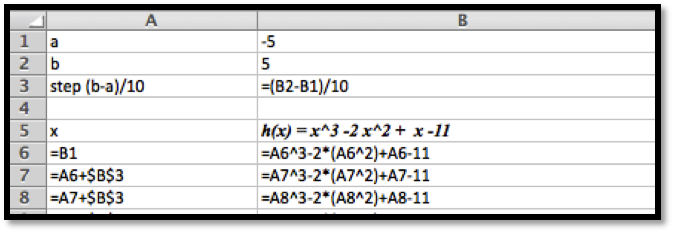
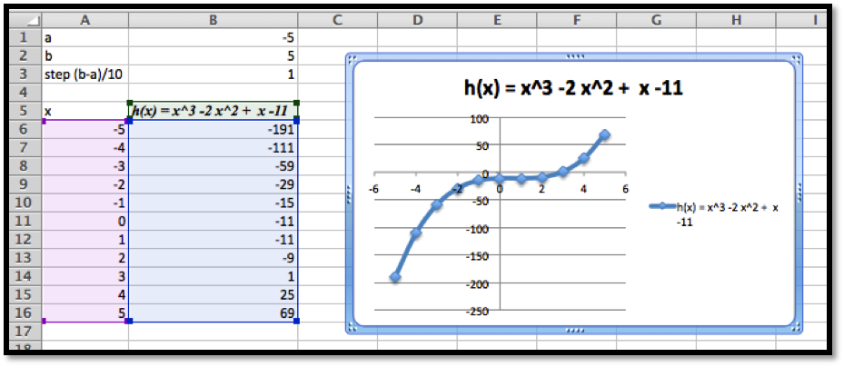
Produce a worksheet with a graph of (h(x) = x^3 -2 x^2 + x -11) for (x) going from a to b, where the values of (a) and (b) can be changed and the graph will update automatically. For initial values, use (a = -5) and (b = 5text<.>)
The entries are (a) and (btext<,>) and the step size. We assume here that we are using 10 points to create a graph.
The data and the graph looks as follows, and changing (a) and (b) allows us to quickly find several different graphs of the same function.
Produce a worksheet with a graph of (k(x) = (x^2 -5 x + 2)/( x -11)) for (x) going from (a) to (btext<,>) where the values of a and b can be changed and the graph will update automatically. For initial values, use (a = -5) and (b = 5text<.>)
(Writing assignment) Write a report of 2 pages or less on the graph of the function (f(x) = (x^2 + 7 x + 10)/(x^2 — 3 x +2)text<.>) The report should be in Word (or other word processor) format with at least 2 graphs that illustrate different features by looking at different viewing windows.
Produce a worksheet with graphs of (f(x) = 2 x + 5) and (g(x) = x^3 — 9 xtext<,>) for x going from -10 to 10. Use secondary axes so that both graphs use the full plotting window.
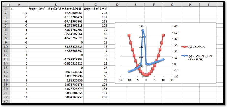
Produce a worksheet with graphs of (h(x) = (x^3 — 9 x)/(x^2 + 3 x + 35/16)) and (k(x) = 2 x^2 + 5text<,>) for x going from -10 to 10. Use secondary axes so that both graphs use the full plotting window. Adjust the range of (y) values used to make the graph reasonable.
The entries should look like this:
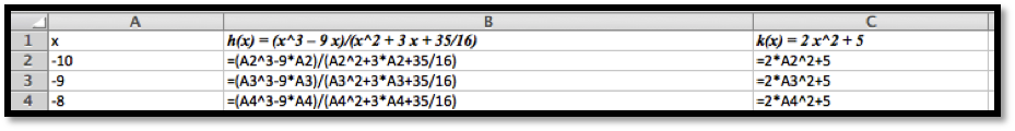
Using secondary axes we are able to show the important feature of each of the graphs.
Produce a worksheet with graphs of (f(x) = 2 x + 3) and (g(x) = -2 x +5text<,>) for (x) going from -10 to 10. Add a title to the chart. Do something interesting with the fonts or other options and explain what you did.
Use Wolfram Alpha to produce a graph of (f(x) = x^3 — 16 xtext<,>) for (x) going from -5 to 5. Use your favorite screen capture software and paste the result into an Excel worksheet.
Using Wolfram, the command and the resulting graph look like this:
Источник
When you want to graph a function, you need to take into account how the data you are using to graph the function is organized. This means that you have to think about the shape of the graph, where the graph’s relative extrema are, and how to calculate the slope of the graph.
Method to Calculate the slope of a Function
To calculate the slope of a function, you first need to know its y-intercept. This is the point on the line where the line crosses the y axis, but does not pass through it. If you have a horizontal line, the y-intercept is the y axis.
The y-intercept can be calculated with the equation y = 3x – 6. A positive y-intercept is when the line crosses the y axis, while a negative y-intercept is when it doesn’t.
The slope of a line is a measure of how steep it is. A positive slope is when the direction is to the right, and a negative slope is when the direction is to the left.
Slope is also measured by the number of steps a person takes while moving in the positive or negative direction. For example, a person moving from Point One to Point Two takes four steps in the positive direction and two in the negative.
A good way to calculate the slope of a function is to use the slope formula. This formula can be used to calculate the slope of a vertical line, a horizontal line, or any other linear function.
Identifying the shape of the Function graph
A graph of a function is a great way to visualize the equation. It can also show how the function is changing, whether it is up or down. It can even solve an equation. This article will help you identify the shape of the graph of a function.
There are several ways to create a graph of a function. One method is to draw a line on the graph and then find the point on the x-axis that matches the y-value of the point. You can also use a table of values to draw the graph. However, it is often easier to do it by hand.
If you don’t have access to a calculator, you can use the Graphical Function Explorer to make a graph of a function. The app allows you to enter a function, select one of three functions, and then plot them. In the process, you can see how the y-values change as the x-values change.
While the vertical line test can be helpful, it does not tell you much about the shape of the graph. When you add a second derivative to the equation, you get the real shape of the graph. For example, the y-value at the point where the vertical line intersects the graph represents the output for the x value.
Creating a scatter plot
When you graph a function, you can choose a scatter plot, which shows a correlation between two variables. In a scatter plot, the data points are scattered around the graph. The vertical axis indicates the direction of the relationship.
A scatter plot can be created in R using the plot() function. This function accepts the main parameter and two parameters for horizontal and vertical coordinates.
To create a scatter plot, you must input data in two columns. Each column should have a value on the x-axis and a value on the y-axis. You can also add a third variable to the plot.
Creating a scatter plot is similar to creating a line graph. However, the scatter plot is more suited to smaller data sets. If you have large data sets, you may prefer a bar chart.
For your scatter graph, you will need to decide on the size of your marker. These markers are used to mark the points. You can either change the color of the marker on the graph, or you can choose to use a transparent data point.
Finding the exact location of a function’s relative extrema
A function’s relative extrema tells you where a function’s maximum or minimum value is located. If the function has a global extremum, then you can find it by equating the first derivative to zero and setting the second derivative to 0. However, if you want to find the local extrema of a function, then you need to find critical numbers and then graph them to see where the function’s extreme values are.
The absolute extremum of a function is an extreme point relative to all points within an interval. For example, the maximum height of a hill is a relative max. It does not have to be the highest peak.
Relative minima are the points at the bottom of a valley. They are also the top of a hill. These are the minimum values that are at least as small as the other values around them.
Absolute minima, on the other hand, are the smallest values of x and y. They are 0 at x=0, and t/16 – 2 at x=t/16.
When you are graphing a function, you can detect the relative extrema by looking for valleys and peaks. These are the places where the function’s increasing and decreasing behavior changes. In fact, these are the places where the function’s turn points are. You can also check for changes in the first and second derivatives of the function at these points.
Adding data labels in a Graph
Data labels are used to identify data series in a graph. They help the audience understand the information better. You can add and remove them easily. Excel allows you to use custom formulas to create and modify them. The formulas can automatically update them as data changes on your worksheet.
Data labels can be added to a chart and you can also change the size, font, and color. Labels are shown in the base of the graph, to the left of the text, and above the graph. By default, the labels are tied to your worksheet values. But you can remove them by right-clicking on them. If you want, you can move them horizontally or vertically to a more convenient location.
Read Also: How To Calculate The Angular Velocity Formula
To add a data label to a chart, select the data point in which you want to place the label. Alternatively, you can double-click on the point to open the Plot Details dialog. After a data point is selected, click the Add Data Labels button in the Context Menu.
When you add a label, you can specify the column of labels you want to use. For example, you can choose one series or all series. You can even set the text style, font, and size to a particular value.
Once you’ve added a label to a chart, you can remove it by right-clicking it. However, you cannot delete data labels that are already in the graph.
Learning how to graph functions in Excel can be daunting, but it is a good skill to learn. Luckily, Excel has many wonderful features that make the process easy to learn and use. This article outlines the process with step-by-step instructions to help you graph functions in Excel in no time.
We’ll go over what graph functions are, discuss the top reasons you should learn how to graph functions in Excel, and show you the benefits of using this software program. This detailed step-by-step guide will have you using Excel like a pro.

Find Your Bootcamp Match
- Career Karma matches you with top tech bootcamps
- Access exclusive scholarships and prep courses
Select your interest
First name
Last name
Phone number
By continuing you agree to our Terms of Service and Privacy Policy, and you consent to receive offers and opportunities from Career Karma by telephone, text message, and email.
What Are Graph Functions in Excel?
Graph functions in Excel are preset formulas used to determine an output variable using input variables. This function calculates the necessary variables you want to define and uses them to display the data visually on a graph or chart.
Graph functions make it easier for businesses to track their performance and predict possible future sales, solutions, and problems. This tool allows you to make statistical calculations quickly and creates a visual representation of complex data.
Why Learning How to Graph Functions in Excel is Useful
- Excel Helps You Visualize Your Data Quickly. Excel has a wide variety of helpful functionalities that can execute simple or complex calculations. You can use it to turn your function and data into a graph or dynamic chart in only a few simple steps.
- You Can Improve and Gain Excel Skills. Many businesses use Excel to perform complex and day-to-day tasks. Learning how to graph functions in Excel will develop your Excel skills which can open up more opportunities for you to get promoted or apply for higher-paying jobs.
- Excel Helps You Learn Which Graph to Use. There are many graph types in Excel you can choose from such as column graphs and bubble charts. Trying different chart options will help you understand which are the best graphs to use for the kinds of data you want to display. One scenario might call for a bubble chart, while another requires a scatter chart.
- You Can See Your Data in a New Way. Graphing functions in Excel can help you see your data in a new light. This can help you view your data differently and see any problems with the data set that you may have missed before. You can add trendlines on charts to ensure they are easy to interpret.
How to Graph Functions in Excel: A Step-By-Step Guide
Step 1: Write Down the Headers
Open the program and create a new worksheet to start your graph function in Excel. First, you’ll need to write your headers into cells. These headers will determine your input and output columns. You can either name them “x” and “y”, or you can be specific and name them “sales” and “profit”, for example. Cell A1 is your input column, cell B1 is your output column.
Step 2: Insert Your Input Variables
Now, you need to enter the values for the horizontal x-axis. Start by typing the first value in cell A2, the next value in cell A3, and continue in that column until every input variable is written. Select all the values in the input column by dragging the cursor down until you have selected them all, open the “Formula” tab at the top of the page, and click “Define Name”. Write the “x” in the name box and click “OK”.
Step 3: Enter your Formula
You’ll then need to write the formula into cell B2 for your graphing function. Start by writing the “=” symbol in the B2 cell followed by the formula. Don’t leave any spaces after the “=” or else the formula won’t work.
For example, if you want to find out what levels of sales you need to break even, write “=(A2*50)-2500” in the cell. The “*” symbol represents multiplication, the number 50 is for the cost of each product and 2500 is what you paid for the products and advertising costs. You can use this calculation method to track anything.
Step 4: Put the Formula Into the Output Column
Now that your formula is written out and ready to use, copy the formula you have written in cell B2 by clicking on it and selecting the “Copy” icon at the top of the Home tab. Select all of the cells in your output column starting with cell B3, then select the arrow on the “Paste” option and click on “Formulas” to paste the formula into the cells of your current selection. You should end up with a value in each cell up to the column up to the last input and output variable.
Step 5: Create Your Graph
With all the difficult work done, you can now create your graph. Select all the cells in your worksheet containing variables, including the headers in your selection. Open the “Insert” tab, go to the “Chart” menu and select the type of graph you want to use out of the many options you have available.
You can go for a scatter plot with smooth lines, a column chart, or any other chart type that will work with your data set. You can also use a trendline to make data trends more obvious. Excel has several trendline options.
Benefits of Graph Functions in Excel
- It’s Easy to Learn and Use. Many industries use Excel because it’s simple, widely available, and equally easy to access and understand for people. Microsoft has many training videos, and other establishments offer fantastic online Excel courses and training that can show you how to graph functions and use all of its other functionalities.
- It Lets You Identify Trends and Issues. Looking at raw data or even data in a table can sometimes be challenging to interpret. Using Excel to graph functions can help you better assess business trends and possible problems.
- It Lets You Easily Create Data-Driven Reports. Excel is a fantastic software with many formulas and functions you can use to easily graph functions the data you enter into a table.
- It Has Plenty of Customization Options. Excel allows you to quickly and easily customize your table and individual chart elements. You can customize your chart title and chart style and change a graph after you’ve made it if you need to.
- It’s Cheap. Microsoft 365, which comes with Excel, costs around $6 to $9 per month, depending on whether you buy it for personal or business use. It’s a cost-effective program considering everything you can do on it.
Importance of Learning How to Use Excel Sheets
Learning how to use Excel sheets is essential for many professionals. Excel’s automated functionalities make admin and data entry and analysis jobs much easier. According to Statista, over one million companies use Office 365. Learning how to use this program will make you a valuable asset to your company. Learning how to use Excel can also open you up to job opportunities due to the sheer number of them that use it.
If you want to broaden your horizons and learn how to use Excel sheets, you can enroll in an Excel bootcamp. Bootcamps are short-term, intensive learning programs that can teach you all you need to know about a specific topic.
How to Graph Functions in Excel FAQ
Can you add multiple functions to one graph?
Yes, you can add more functions to a graph after creating the first. First, go to “Chart Tools” and select the “Design” tab, then click the “Select Data Source” button. Add your new variables by clicking “Add” below the “Series” option. There, you can add the new variables and press “OK” to finish the process.
How do I add a title to my graph in Excel?
You can add a heading to your graph in excel by following simple steps. Click the “Chart Title” option and type in your header when you are on the chart. Next, click on the + symbol at the top-right of the graph and select the arrow. Click on Centered Overlay, and your title should appear on your graph.
What professions use Excel often?
Professions that use Excel include sales managers, quality analysts, economists, construction managers, and statisticians, among many others. There is a wide range of jobs that use Excel skills.
Why is a graph better than looking at raw data?
Using a graph to represent data is much better than looking at raw data because a graph is easier to understand and interpret.
A mathematical function is a formula that takes an input, x, applies a set of calculations to it, and produces an output called y. By calculating a function at a large number of set intervals, it is possible to create a scatter plot of a function. In business this has many uses. For example, you can plot profit minus costs at various levels of sales, or total costs can be estimated by plotting fixed costs at different increments of variable costs.
-
Create the headers for your data table. Enter the input variable in cell A1 and the output variable in cell B1. If you like, you can use the mathematical standards «x» and «y,» or you can use something more descriptive such as «sales» and «profit.»
-
Enter the first and second interval of your input variable (for example, «x» or «sales»), which you’ll use to plot the function. For example, if your intervals are whole numbers, you might start by entering «1» into cell A2 and «2» into cell A3. Select both of these cells and then click and drag the small black square in the lower-right corner of the selection area downwards until you have as many values as you want to plot.
-
Type an equal sign «=» into cell B2 and then type your formula directly after it, without leaving a space. For example, to determine the number of sales you need to make of a certain product to cover costs, you could use:
=(A2*50)-3500
Replace «50» with your sale price and «3500» with your costs.
-
Select cell B2 and then drag to copy the formula down the column with the same method you used in step 2. Make sure each of your x values has a corresponding function to the right of it. As you do this, the column will automatically populate with the solutions to each function, based on the value of x in column A.
-
Select all the cells you have entered data into, including your header.
-
Click the «Insert» tab, click «Scatter» in the Charts area and then click the type of graph you need. The graph will then appear on your worksheet.