
![]()
Download Article
In-depth guide for opening Excel files on your PC or phone
![]()
Download Article
This wikiHow teaches you how to open an Excel file, and view the spreadsheet file’s contents. You can use a desktop spreadsheet program like Microsoft Excel, a web-based spreadsheet viewer like Google Sheets, or the mobile Excel app to open, view, and edit Excel spreadsheets on any computer, phone or tablet.
-

1
Find and right-click the Excel file you want to open. Find the spreadsheet file on your computer, and right-click on its name or icon to see your options on a drop-down menu.
-
2
Hover over Open with on the right-click menu. A list of available apps will pop up on a sub-menu.
Advertisement
-
3
Select Microsoft Excel on the «Open with» menu. This will launch Excel on your computer, and open the selected file.
- If you don’t see the Excel app here, click Other or Choose another app to see all your apps.
- If you don’t have Excel installed, check out the available subscription plans and get a free trial at https://products.office.com/en/excel.
- As an alternative, you can download and use a free, open-source office suite like Apache OpenOffice (https://www.openoffice.org) or LibreOffice (https://www.libreoffice.org).


Advertisement
-
1
Open Microsoft Excel Online in your internet browser. Type or paste https://office.live.com/start/Excel.aspx into the address bar, and press ↵ Enter or ⏎ Return on your keyboard.
- If you’re prompted, sign in with your Microsoft ID or Outlook account.
- You can use Excel online in any desktop or mobile internet browser.
-
2
Click the Upload a Workbook button on the top-right. This button looks like a blue, upwards arrow icon in the upper-right corner of the page. It will open your file navigator, and allow you to select a file from your computer.
-
3
Select the Excel file you want to open. Find your spreadsheet file in the file navigator window, and click on its name or icon to select it.
-
4
Click Open. This button is in the bottom-right corner of the file navigator pop-up. It will upload your spreadsheet file, and open it in Excel Online.
- You can view and edit your file in your internet browser.


Advertisement
-
1
Open Google Sheets in your internet browser. Type or paste https://docs.google.com/spreadsheets into the address bar, and press ↵ Enter or ⏎ Return on your keyboard.
- Alternatively, go to https://sheets.google.com. It will open the same page.
- If you’re not automatically signed in, log in with your Google account.
- You can use Google Sheets in any desktop or mobile internet browser.
-
2
Click the folder icon on the top-right. You can find this button in the upper-right corner of your spreadsheet list, next to the AZ button. It will open the «Open a file» window in a pop-up.
-
3
Click the Upload tab. You can find it on a tab bar below the «Upload a file» heading in the pop-up. This will allow you to open any Excel file from your computer.
- Alternatively, you can click the My Drive tab, and open a file from your Google Drive library.
-
4
Drag and drop your Excel file on the «Open a file» window. When you’re in the Upload tab, you can just drag and drop any spreadsheet file from your computer here.
- This will upload your Excel file to Google Sheets, and open it in your internet browser.
- Alternatively, click the blue Select a file from your device button, and select your file manually.


Advertisement
-
1
-
2
Tap Sign in later at the bottom. This option will allow you to use the mobile Excel app on your phone or tablet without signing in to your Microsoft account.
- Alternatively, enter your registered email, phone or Skype ID, and tap the green-and-white arrow to sign in to your account.
-
3
Tap the Open button. This button looks like a folder icon on a navigation bar. It will open your available file sources.
- On iPhone, it’s in the lower-right corner of your screen.
- On Android, it’s in the upper-left corner of your screen.
-
4
Select where your spreadsheet file is saved. Selecting a source here will open all the files saved to this location.
- If you’re opening a file saved to your phone or tablet’s local storage, select This Device or On My iPhone/iPad here.
-
5
Select the spreadsheet file you want to open. Tapping a file will open it in the Excel mobile app.


Advertisement
Ask a Question
200 characters left
Include your email address to get a message when this question is answered.
Submit
Advertisement
Thanks for submitting a tip for review!
About This Article
Article SummaryX
1. Find and right-click the file.
2. Hover over Open with.
3. Select Microsoft Excel.
Did this summary help you?
Thanks to all authors for creating a page that has been read 63,704 times.
Is this article up to date?
Lesson 1: Getting Started with Excel
Introduction
Excel is a spreadsheet program that allows you to store, organize, and analyze information. While you may think Excel is only used by certain people to process complicated data, anyone can learn how to take advantage of the program’s powerful features. Whether you’re keeping a budget, organizing a training log, or creating an invoice, Excel makes it easy to work with different types of data.
Watch the video below to learn more about Excel.
About this tutorial
The procedures in this tutorial will work for all recent versions of Microsoft Excel, including Excel 2019, Excel 2016, and Office 365. There may be some slight differences, but for the most part these versions are similar. However, if you’re using an earlier version, you may want to refer to one of our other Excel tutorials instead.
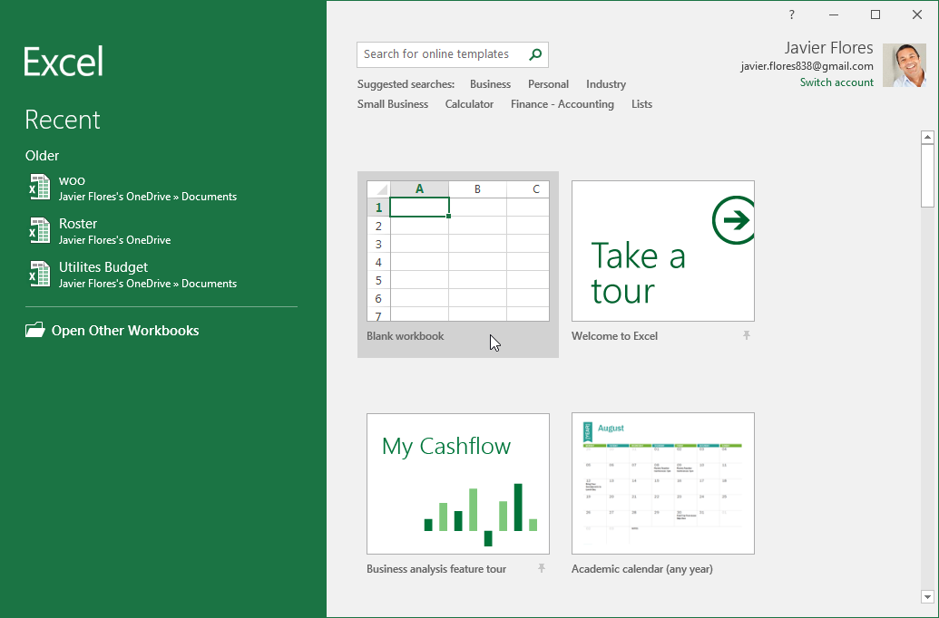
The Excel Start Screen
When you open Excel for the first time, the Excel Start Screen will appear. From here, you’ll be able to create a new workbook, choose a template, and access your recently edited workbooks.
- From the Excel Start Screen, locate and select Blank workbook to access the Excel interface.

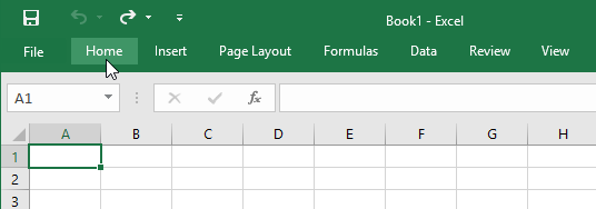
The parts of the Excel window
Some parts of the Excel window (like the Ribbon and scroll bars) are standard in most other Microsoft programs. However, there are other features that are more specific to spreadsheets, such as the formula bar, name box, and worksheet tabs.
Click the buttons in the interactive below to become familiar with the parts of the Excel interface.
Working with the Excel environment
The Ribbon and Quick Access Toolbar are where you will find the commands to perform common tasks in Excel. The Backstage view gives you various options for saving, opening a file, printing, and sharing your document.
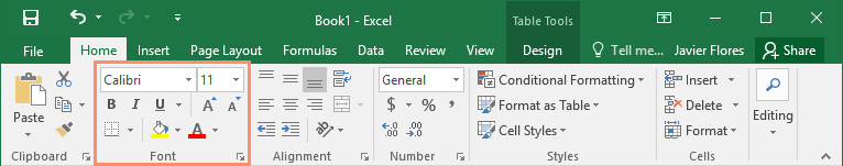
The Ribbon
Excel uses a tabbed Ribbon system instead of traditional menus. The Ribbon contains multiple tabs, each with several groups of commands. You will use these tabs to perform the most common tasks in Excel.
- Each tab will have one or more groups.
- Some groups will have an arrow you can click for more options.
- Click a tab to see more commands.
- You can adjust how the Ribbon is displayed with the Ribbon Display Options.
Certain programs, such as Adobe Acrobat Reader, may install additional tabs to the Ribbon. These tabs are called add-ins.
To change the Ribbon Display Options:
The Ribbon is designed to respond to your current task, but you can choose to minimize it if you find that it takes up too much screen space. Click the Ribbon Display Options arrow in the upper-right corner of the Ribbon to display the drop-down menu.
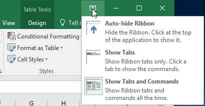
There are three modes in the Ribbon Display Options menu:
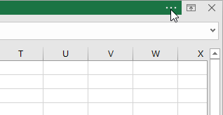
- Auto-hide Ribbon: Auto-hide displays your workbook in full-screen mode and completely hides the Ribbon. To show the Ribbon, click the Expand Ribbon command at the top of screen.
- Show Tabs: This option hides all command groups when they’re not in use, but tabs will remain visible. To show the Ribbon, simply click a tab.
- Show Tabs and Commands: This option maximizes the Ribbon. All of the tabs and commands will be visible. This option is selected by default when you open Excel for the first time.
The Quick Access Toolbar
Located just above the Ribbon, the Quick Access Toolbar lets you access common commands no matter which tab is selected. By default, it includes the Save, Undo, and Repeat commands. You can add other commands depending on your preference.
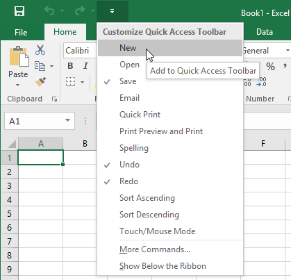
To add commands to the Quick Access Toolbar:
- Click the drop-down arrow to the right of the Quick Access Toolbar.
- Select the command you want to add from the drop-down menu. To choose from additional commands, select More Commands.
- The command will be added to the Quick Access Toolbar.
How to use Tell me:
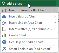
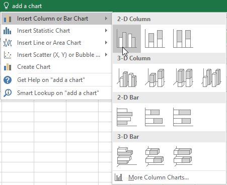
The Tell me box works like a search bar to help you quickly find tools or commands you want to use.
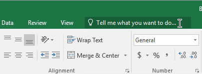
- Type in your own words what you want to do.
- The results will give you a few relevant options. To use one, click it like you would a command on the Ribbon.
Worksheet views
Excel has a variety of viewing options that change how your workbook is displayed. These views can be useful for various tasks, especially if you’re planning to print the spreadsheet. To change worksheet views, locate the commands in the bottom-right corner of the Excel window and select Normal view, Page Layout view, or Page Break view.
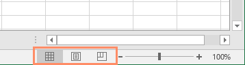
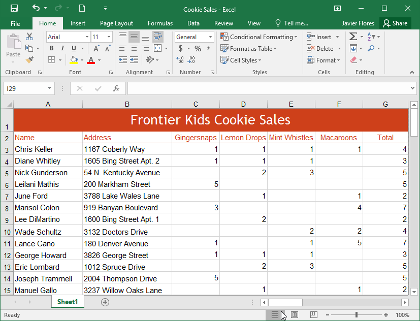
- Normal view is the default view for all worksheets in Excel.

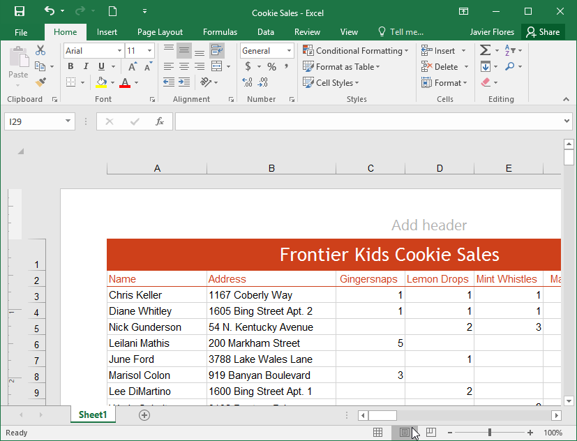
- Page Layout view displays how your worksheets will appear when printed. You can also add headers and footers in this view.
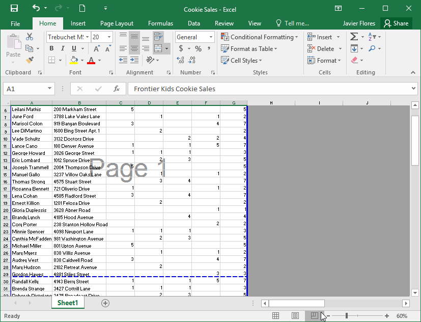
- Page Break view allows you to change the location of page breaks, which is especially helpful when printing a lot of data from Excel.
Backstage view
Backstage view gives you various options for saving, opening a file, printing, and sharing your workbooks.
To access Backstage view:
- Click the File tab on the Ribbon. Backstage view will appear.
Click the buttons in the interactive below to learn more about using Backstage view.
Challenge!
- Open Excel.
- Click Blank Workbook to open a new spreadsheet.
- Change the Ribbon Display Options to Show Tabs.
- Using the Customize Quick Access Toolbar, click to add New, Quick Print, and Spelling.
- In the Tell me bar, type the word Color. Hover over Fill Color and choose yellow. This will fill a cell with the color yellow.
- Change the worksheet view to the Page Layout option.
- When you’re finished, your screen should look like this:
- Change the Ribbon Display Options back to Show Tabs and Commands.
- Close Excel and Don’t Save changes.
/en/excel/understanding-onedrive/content/
Office 365
The easiest way to get started with Excel, is to use Office 365.
Office 365 does not require downloading and installation of the program. It simply runs in your browser.
In our tutorial we will use Office 365, which can be accessed from www.office.com.
Install
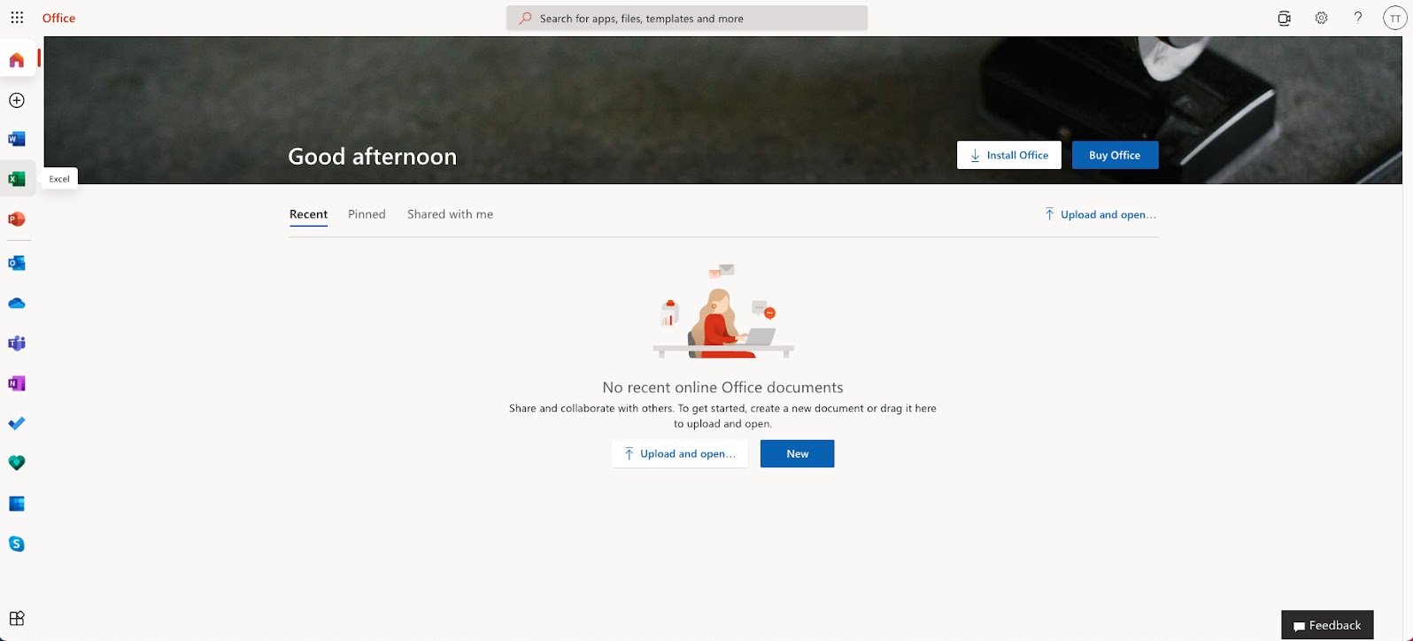
Once you have successfully logged into Office through www.office.com,
click on the Excel icon on the left side to enter the application:
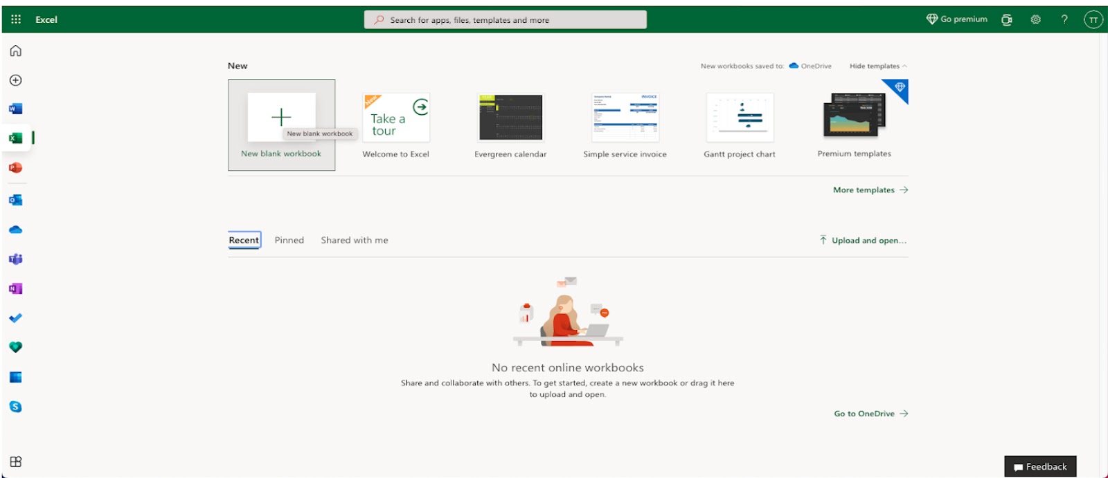
After entering the Excel application, click on the New blank workbook button to get started with a new workbook.
Enter a name for your workbook, and hit the enter button:
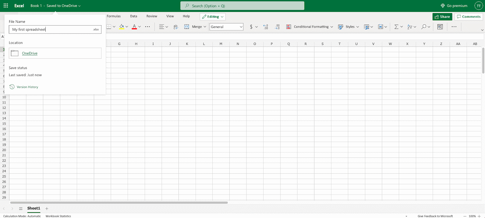
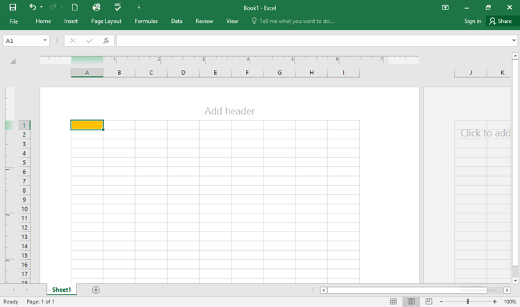
The Excel view has columns and rows, similar to a squared math exercise book.
Do not worry if the functionality looks overwhelming at first. You will get comfortable as you learn more in the chapters to come.
For now focus on the rows, columns, and the cells.
Ok. Let’s make a function!
- First, double click the cell
A1, the one that is marked with the green rectangle in the picture. - Second, type
=1+1. - Third, hit the enter button:
Congratulations! You have typed your first function,
1+1=2.
Launching the Excel Application
Upon starting the Excel application, you are presented with what is known as the Getting Started page.
This page serves as a branching off point to start or access many different types of Excel files. These include, but are not limited to:
- Starting a brand new blank workbook. This is where you begin when you are starting from zero.
- Starting a brand new workbook based on a template. Templates provide an existing framework with labels, formulas, and sample data. Templates are great if you are in a hurry or lack the needed skills to produce the needed output, such as Pivot Tables or Charts.
- Starting a file from the history list. This is a convenient way to open a file you have been working on in the recent hours or days without having to manually locate the file.
- Open a file not in the history. This is useful for files you may have downloaded from email attachments or recently gained access to via a USB device.

Starting a New, Blank Workbook
When you begin with a new, blank workbook, the workbook is not saved until you initially save the file.
To save the workbook, click the Save button in the Quick Access Toolbar (upper-left corner), provide a name and location to save the file, and click Save. You can also use the keyboard shortcut CTRL-S.

A single Excel file is often referred to as a workbook or spreadsheet. A workbook consists of at least one sheet.

Additional sheets can be added by clicking the “plus” button to the right of the sheet tabs.

You can rename a sheet by double-clicking on the sheet tab to enable rename mode.

The Layout of the Grid
Each sheet in a workbook is composed of a series of rows and columns. Where these rows and columns interest we have what are called cells.

Each sheet has the following dimensions:
- Columns = 16,384
- Rows = 1,048,576
- Cells = 17,179,869,184
This means you can place over 17 billion pieces of unique information on a single sheet.
Entering Data into a Cell
To enter information into a cell, click on the desired cell and start typing. If the cell began as an empty cell, the newly entered data will be displayed. If the cell contains information, that information will be replaced with the newly entered data.
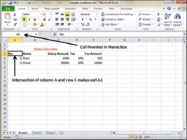
Cell Addresses
Each of the over 17 billion cells on a sheet has a unique address. The address is a composite of the cell’s column position (a letter) and the cell’s row position (a number).

The Formula Bar
The Formula Bar is where formulas, numbers, or text can be edited after being placed in a cell.

Although you can edit the contents of a cell directly on the grid, this becomes more challenging when working with complex formulas or long passages of text. Performing the edits in the Formula Bar will prove a much easier task.
A cell containing numbers or text will display the same information on the Formula Bar as is displayed in the cell.
A cell that contains a formula will display the formula in the Formula Bar and the formula’s result in the cell.
The Name Box
The Name Box serves several purposes. One purpose is to display the address of the currently selected cell.

This will make it easier to accurately determine the address of the selected cell, especially if you happen to be zoomed out to a point where reading the row and column headings become difficult.
“Teleporting” to a Cell
When you need to position yourself in a cell that is a considerable distance from your current location, you can type the address of the destination cell into the Name Box and press Enter. This will instantly relocate you to the new cell.
Try the following cell address to see the end of the spreadsheet universe (lower-right corner of the sheet.)

To return to the “beginning” of the sheet (upper-left corner of the sheet) enter the cell address A1 into the Name Box and press Enter. You can also press the CTRL-Home keys to instantly relocate to cell A1.
Selecting Single/Multiple Rows & Columns
To select a row or column, click the applicable row or column header.

To select multiple rows or columns, click and hold the first row/column, then drag across the adjacent rows/columns until you have selected all the needed locations.
Shortcuts Galore
Excel has more shortcuts than probably anyone knows (at least anyone with a social life.)
One of the best shortcuts for selecting columns is CTRL-Space.

With the column selected, holding the Shift key while repeatedly pressing the left/right arrow keys will select multiple adjacent columns.
NOTE: If you want to see a demonstration of many of the most popular Excel keyboard shortcuts, check out this post and video:
Useful Excel Shortcuts
When you right-click a cell, you will receive a menu of options. The options displayed are directly related to the object you have right-clicked on.

With selected columns or rows, clicking the Insert or Delete options in the right-click menu will either add or remove columns or rows in the same quantity selected.
Coolest Way to Add/Remove Rows & Columns
When you select a row or column, or a series of rows or columns, you can press the CTRL-plus or CTRL-minus keys to quickly add or delete rows or columns.
It is likely to be easier to perform this using the plus/minus keys on the numeric keypad. If you use the plus/minus button located above the letter keys, you will have to add the extra step of using Shift when using the plus key.
Moving to the Extents of the Sheet or Data
You can use the CTRL key along with the up/down/left/right arrow keys to navigate to the extent of the sheet, or if you have existing data, the extent of the data range.

Defining Ranges of Cells
An important term to understand is the word Range. A Range is either a single cell or a group of cells.
When we define a range in a formula, we always refer to the range starting from the upper-left corner of the range to the lower-right corner of the range. We place a colon between the two range addresses to symbolize the word “through”.
Selecting and Moving Cells
When you move your pointer around the grid, you will see a large white plus symbol known as the General Select symbol.

Placing this symbol in the center of a cell and clicking will select the designated cell.
If you place your General Select symbol in the green edge of the selected cell, you will see the large, white plus change to a thinner, black directional arrow known as the Move icon.

If you click and drag from the green border, you will move the selected cell or range of cells.
If you need to move data between sheets, workbooks, or great distances on the same sheet, you can use the traditional Cut-Paste technique.
The Fill Series Handle
One of the greatest data entry time-savers is the Fill Series handle.

When you place your pointer over this green handle, your large, white plus symbol will change to a thin, black plus symbol.

When you see this symbol, click and drag it down or to the right to invoke the Fill Series feature.
Below is a shortlist of things the Fill Series feature will perform:
- Repeat text
- Create lists of months
- Create a list of weekday names
- Create lists of days
- Repeat formulas
- Repeat cell formatting

Resizing Rows and Columns
If you require more width for your columns (typically for text entries), you can hover your pointer over the right column divider (i.e., the divider between columns D & E to resize column D) and click to drag the divider left or right as needed.

You can perform the same operation on rows by selecting the bottom divider for a specific row and drag up and down as needed.
If you place your pointer over a column or row divider and double-click the mouse, you can invoke an “Auto-Fit” command. This will enlarge or shrink the row/column to the optimal size based on the data contained on that row or column.
Wrapping Text within a Cell
If you don’t want to have an overly wide column to accommodate the contained text, you can activate the Wrap Text feature to have the text automatically apply in-cell carriage returns based on the data and the size of the cell.

You can remove this feature by selecting the wrapped text cell and clicking the Wrap Text button to toggle the feature to the off state.
Touring the Ribbon
The Tabs and the Ribbon provide access to many of the program’s features.

Clicking the various Tabs will reveal collections of similarly purposed features.
Most of the structural changes made to sheets, like paper size, margin sizes, paper orientation are found on the Page Layout ribbon.

The most used features of the program are located on the Home tab/ribbon.
Learning About Buttons
If you are unsure as to what a particular button will do for you, you can hover your pointer over the button to reveal the “Tell me more” information.

This provides a brief explanation of the button’s purpose, its keyboard shortcut key sequence (if applicable), and a link to open the official Microsoft documentation page for the feature.
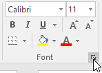
Accessing the “Deep Dive” Features
Many of the Ribbon groupings have more features than can be displayed without making the Ribbon overly complicated. For these lesser-used features, you can click the “additional options” button located in the lower-right corner of the button group.

These will open various dialog boxes that contain additional features related to the button group’s overall purpose.
Giving More Space to the Grid
If you want to give more screen space to the grid (and less to the Ribbon), you can either click the “Collapse the Ribbon” button (upper-right corner) or press the CTRL-F1 key combination.

The Ribbon will be hidden leaving only the Tabs visible.

The Ribbon is still accessible by clicking a Tab, but it will automatically hide once it has served its purpose.
NOTE: You can also double-click a Tab to apply or remove this auto-hide behavior of the Ribbon. Many users “discover” this feature accidentally by double-clicking a Tab and thinking they have just lost their Ribbon. Not to worry; double-clicking a Tab will remedy the situation.
Accessing the Backstage
Clicking the File tab will reveal the Backstage.


The Backstage is where you go to manipulate the file as an object.
What I mean is you are trying to perform actions such as:
- Save the file
- Open a file
- Close a file
- Print a file
- Email the file
- Convert the file (ex: PDF, or delimited text)
- Protect the file (e., password to open or password to edit)
- Obtain file statistics (ex: size, author, creation date, last saved date, etc.)
Shortcuts for Inputting Values
Getting Out of Edit Mode
When entering data, pressing the Tab key will move the cursor right to the next column, while pressing Enter will move the cursor down to the next row.
If you wish to enter the data without relocating the cursor, press CTRL-Enter.
Getting Into Edit Mode
If you need to edit the contents of a cell, you can select the cell and then press the F2 key. This will enable Edit Mode and place your cursor at the end of the cell’s contents.
Repeating Cell Data
If you have text, numbers, or formulas in a cell, select the cell and adjoining cells to the left or below then press either CTRL-R or CTRL-D to repeat the first cell’s contents to the other selected cells either to the right on the row or downward (below) in the column.
Confining the Data Entry Cells
If you know you wish to restrict the data to a set range of rows and columns, you can pre-select the range. By doing so, repeated pressing of the Tab key will confine the cell selections to the pre-selected range.

Formatting Data (Let’s make this pretty!)
We have a set of data where department headcounts are displayed by month.

Attractive Titles
To make the report more attractive, we begin by centering the heading between columns A and G. This is accomplished by selecting the cells you wish to center across (A1 through G1) and press the Merged & Center button.

Resizing Multiple Columns
If you wish to tighten up the space used by the monthly columns (B through G), select the column headings for columns B through G, then double-click one of the highlighted column heading dividers (remember Auto Fit?).

If this is too tight, you can manually expand one of the selected column heading dividers and manually resize to the desired width. This new size will be applied to all selected columns, providing a professional, uniformed look.
Adding Colors and Borders
With the Month cells selected, we can apply any traditional cosmetic changes to the cells, like font style, font size, font color, alignment, etc.
We can also add borders and fill colors to the cells using the Borders and Fill Color features.

Moving Rows (the COOL Way)
Suppose you want to move the order of the Departments in our table above.
Most users would perform the following steps:
- Insert a blank row where they want the data to be moved to
- Select the data to be moved
- Invoke a Cut action
- Select the newly inserted empty row
- Invoke a Paste action (or right-click -> “Insert Cut Cells”)
Although that works, it’s not exactly a crowd-pleasing party trick. Try this instead:
- Select the cells you wish to relocate (ex: A7 through G7).
- Click and hold the border of the highlighted cells (stay away from the Fill Series handle).
- While you drag up or down, press the SHIFT This will reveal a thick green line that indicates the drop location.

Speedy Formatting Trick
If you have a cell that has a certain style (i.e., color, size, font, etc.) and you want all of those same settings applied to other cells, you can use the Format Painter to copy and paste the look of a cell without carrying over the data.

Select the cell that has the style you wish to replicate, click the Format Painter button, then click the cell to which you want to apply the style.
Pro Tip: If you need to apply the style to many cells that may not be in a consecutive arrangement, double-click the Format Painter button to lock it into an “on” state. Select all the needed cells, then click the Format Painter when you’re finished to deactivate the feature or press the ESC key.
Creating Your First Calculations (Adding Values)
If we want to get the monthly totals for all Departments, select the cell below the “Jan” values (cell B8) and press the AutoSum button (or press the ALT-Equals sign) located in the upper-right corner of the Home ribbon.

This will create a formula that uses the SUM function. The formula will attempt to determine the extent of the data. We can easily verify the selection by examining the Marquee (moving dotted line surrounding the selected cells).

Repeating Formulas
If you need to create the same type of formulas for the remaining months, perform the following steps:
- Select the cell with the formula you wish to repeat.
- Place the mouse pointer (thick, white plus symbol) over the Fill Series You should see a thin, black plus symbol.
- Drag the Fill Series handle to the right across the remaining columns of calculations.


Closing Thoughts
Knowing a few of the most used features of Excel will give you the confidence to want to learn more.
The journey to learn Excel is endless, but as with all journeys, it must begin with a few small steps.
Today you walk, tomorrow you run, and soon you will fly.
Published on: February 5, 2021
Last modified: March 24, 2023


Leila Gharani
I’m a 5x Microsoft MVP with over 15 years of experience implementing and professionals on Management Information Systems of different sizes and nature.
My background is Masters in Economics, Economist, Consultant, Oracle HFM Accounting Systems Expert, SAP BW Project Manager. My passion is teaching, experimenting and sharing. I am also addicted to learning and enjoy taking online courses on a variety of topics.
Getting Started with Excel 2010
This chapter teaches you how to start an excel 2010 application in simple steps. Assuming you have Microsoft Office 2010 installed in your PC, start the excel application following the below mentioned steps in your PC.
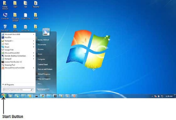
Step 1 − Click on the Start button.
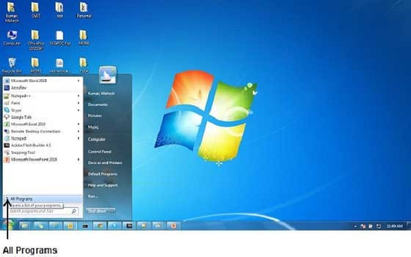
Step 2 − Click on All Programs option from the menu.
Step 3 − Search for Microsoft Office from the sub menu and click it.
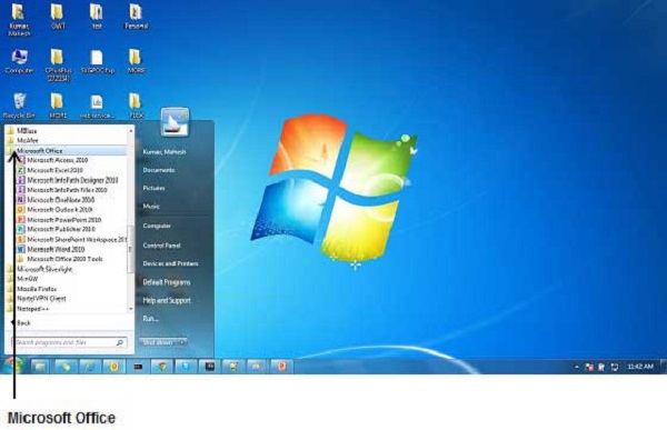
Step 4 − Search for Microsoft Excel 2010 from the submenu and click it.
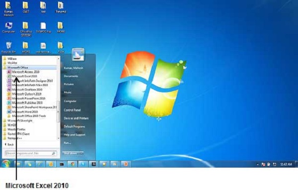
This will launch the Microsoft Excel 2010 application and you will see the following excel window.
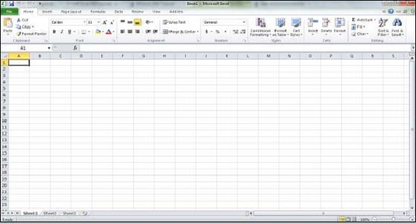
Explore Window in Excel 2010
The following basic window appears when you start the excel application. Let us now understand the various important parts of this window.
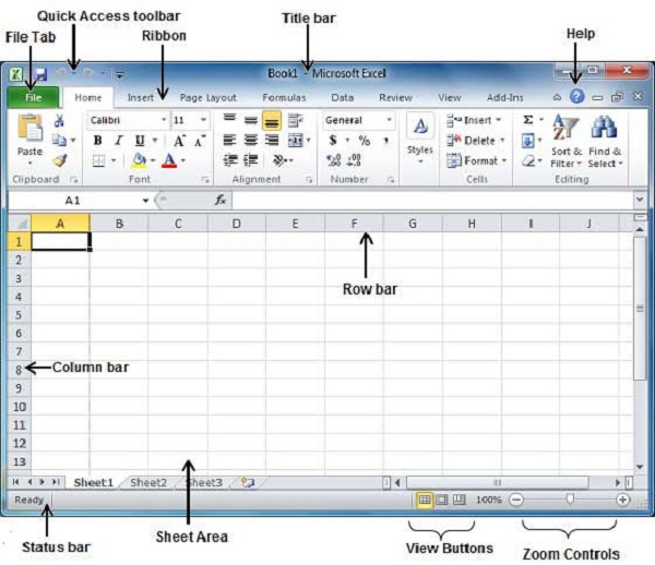
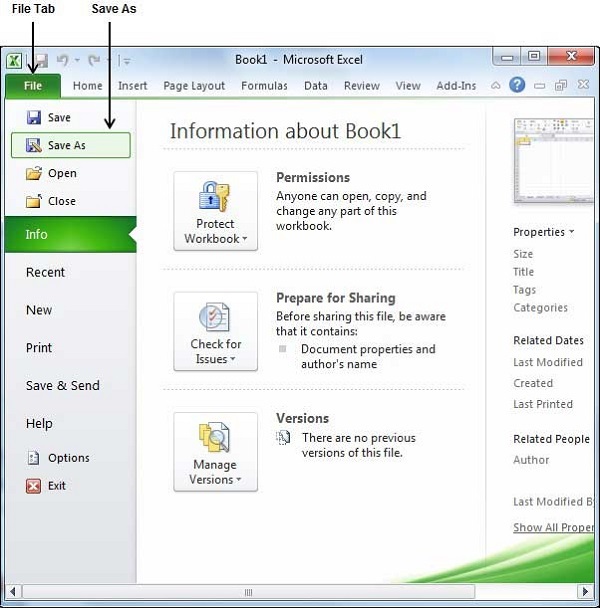
File Tab
The File tab replaces the Office button from Excel 2007. You can click it to check the Backstage view, where you come when you need to open or save files, create new sheets, print a sheet, and do other file-related operations.
Quick Access Toolbar
You will find this toolbar just above the File tab and its purpose is to provide a convenient resting place for the Excel’s most frequently used commands. You can customize this toolbar based on your comfort.
Ribbon
Ribbon contains commands organized in three components −
-
Tabs − They appear across the top of the Ribbon and contain groups of related commands. Home, Insert, Page Layout are the examples of ribbon tabs.
-
Groups − They organize related commands; each group name appears below the group on the Ribbon. For example, group of commands related to fonts or group of commands related to alignment etc.
-
Commands − Commands appear within each group as mentioned above.
Title Bar
This lies in the middle and at the top of the window. Title bar shows the program and the sheet titles.
Help
The Help Icon can be used to get excel related help anytime you like. This provides nice tutorial on various subjects related to excel.
Zoom Control
Zoom control lets you zoom in for a closer look at your text. The zoom control consists of a slider that you can slide left or right to zoom in or out. The + buttons can be clicked to increase or decrease the zoom factor.
View Buttons
The group of three buttons located to the left of the Zoom control, near the bottom of the screen, lets you switch among excel’s various sheet views.
-
Normal Layout view − This displays the page in normal view.
-
Page Layout view − This displays pages exactly as they will appear when printed. This gives a full screen look of the document.
-
Page Break view − This shows a preview of where pages will break when printed.
Sheet Area
The area where you enter data. The flashing vertical bar is called the insertion point and it represents the location where text will appear when you type.
Row Bar
Rows are numbered from 1 onwards and keeps on increasing as you keep entering data. Maximum limit is 1,048,576 rows.
Column Bar
Columns are numbered from A onwards and keeps on increasing as you keep entering data. After Z, it will start the series of AA, AB and so on. Maximum limit is 16,384 columns.
Status Bar
This displays the current status of the active cell in the worksheet. A cell can be in either of the fours states (a) Ready mode which indicates that the worksheet is ready to accept user inpu (b) Edit mode indicates that cell is editing mode, if it is not activated the you can activate editing mode by double-clicking on a cell (c) A cell enters into Enter mode when a user types data into a cell (d) Point mode triggers when a formula is being entered using a cell reference by mouse pointing or the arrow keys on the keyboard.
Dialog Box Launcher
This appears as a very small arrow in the lower-right corner of many groups on the Ribbon. Clicking this button opens a dialog box or task pane that provides more options about the group.
BackStage View in Excel 2010
The Backstage view has been introduced in Excel 2010 and acts as the central place for managing your sheets. The backstage view helps in creating new sheets, saving and opening sheets, printing and sharing sheets, and so on.
Getting to the Backstage View is easy. Just click the File tab located in the upper-left corner of the Excel Ribbon. If you already do not have any opened sheet then you will see a window listing down all the recently opened sheets as follows −
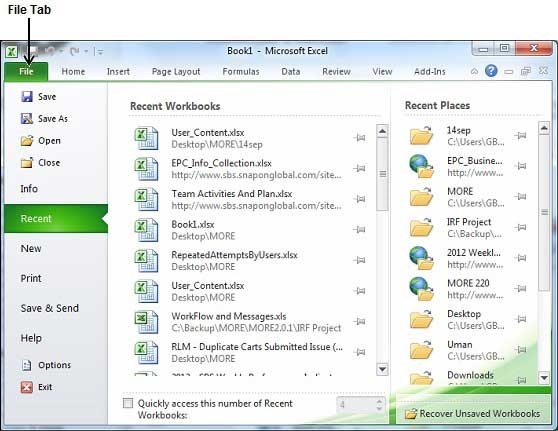
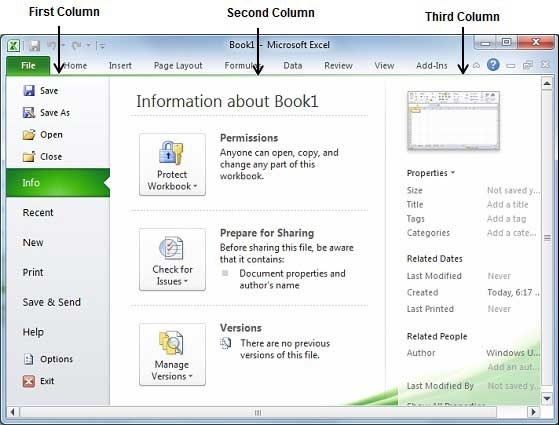
If you already have an opened sheet then it will display a window showing the details about the opened sheet as shown below. Backstage view shows three columns when you select most of the available options in the first column.
First column of the backstage view will have the following options −
| S.No. | Option & Description |
|---|---|
| 1 |
Save If an existing sheet is opened, it would be saved as is, otherwise it will display a dialogue box asking for the sheet name. |
| 2 |
Save As A dialogue box will be displayed asking for sheet name and sheet type. By default, it will save in sheet 2010 format with extension .xlsx. |
| 3 |
Open This option is used to open an existing excel sheet. |
| 4 |
Close This option is used to close an opened sheet. |
| 5 |
Info This option displays the information about the opened sheet. |
| 6 |
Recent This option lists down all the recently opened sheets. |
| 7 |
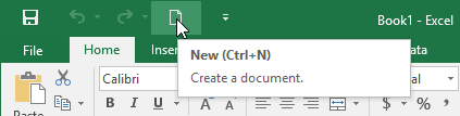
New This option is used to open a new sheet. |
| 8 |
This option is used to print an opened sheet. |
| 9 |
Save & Send This option saves an opened sheet and displays options to send the sheet using email etc. |
| 10 |
Help You can use this option to get the required help about excel 2010. |
| 11 |
Options Use this option to set various option related to excel 2010. |
| 12 |
Exit Use this option to close the sheet and exit. |
Sheet Information
When you click Info option available in the first column, it displays the following information in the second column of the backstage view −
-
Compatibility Mode − If the sheet is not a native excel 2007/2010 sheet, a Convert button appears here, enabling you to easily update its format. Otherwise, this category does not appear.
-
Permissions − You can use this option to protect the excel sheet. You can set a password so that nobody can open your sheet, or you can lock the sheet so that nobody can edit your sheet.
-
Prepare for Sharing − This section highlights important information you should know about your sheet before you send it to others, such as a record of the edits you made as you developed the sheet.
-
Versions − If the sheet has been saved several times, you may be able to access previous versions of it from this section.
Sheet Properties
When you click Info option available in the first column, it displays various properties in the third column of the backstage view. These properties include sheet size, title, tags, categories etc.
You can also edit various properties. Just try to click on the property value and if property is editable, then it will display a text box where you can add your text like title, tags, comments, Author.
Exit Backstage View
It is simple to exit from the Backstage View. Either click on the File tab or press the Esc button on the keyboard to go back to excel working mode.
Entering Values in Excel 2010
Entering values in excel sheet is a child’s play and this chapter shows how to enter values in an excel sheet. A new sheet is displayed by default when you open an excel sheet as shown in the below screen shot.
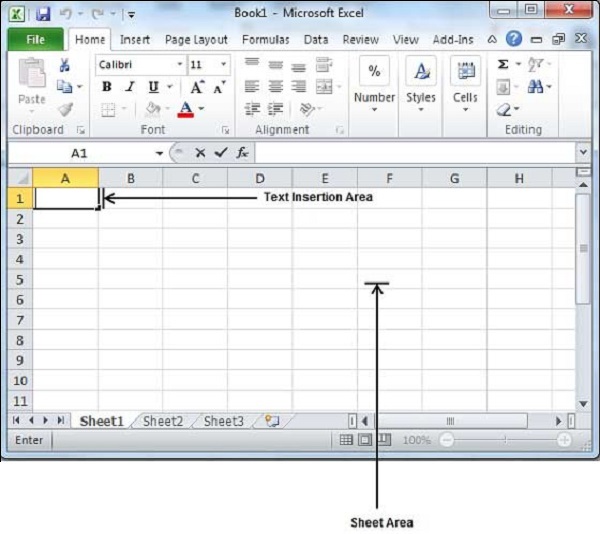
Sheet area is the place where you type your text. The flashing vertical bar is called the insertion point and it represents the location where text will appear when you type. When you click on a box then the box is highlighted. When you double click the box, the flashing vertical bar appears and you can start entering your data.
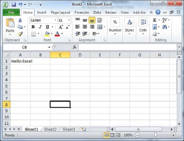
So, just keep your mouse cursor at the text insertion point and start typing whatever text you would like to type. We have typed only two words «Hello Excel» as shown below. The text appears to the left of the insertion point as you type.
There are following three important points, which would help you while typing −
- Press Tab to go to next column.
- Press Enter to go to next row.
- Press Alt + Enter to enter a new line in the same column.
Move Around in Excel 2010
Excel provides a number of ways to move around a sheet using the mouse and the keyboard.
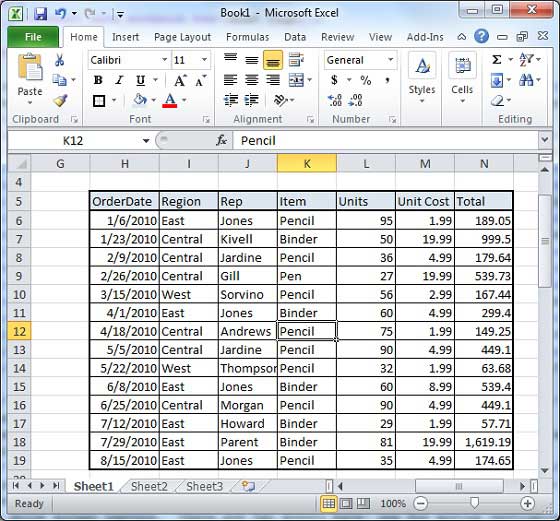
First of all, let us create some sample text before we proceed. Open a new excel sheet and type any data. We’ve shown a sample data in the screenshot.
| OrderDate | Region | Rep | Item | Units | Unit Cost | Total |
|---|---|---|---|---|---|---|
| 1/6/2010 | East | Jones | Pencil | 95 | 1.99 | 189.05 |
| 1/23/2010 | Central | Kivell | Binder | 50 | 19.99 | 999.5 |
| 2/9/2010 | Central | Jardine | Pencil | 36 | 4.99 | 179.64 |
| 2/26/2010 | Central | Gill | Pen | 27 | 19.99 | 539.73 |
| 3/15/2010 | West | Sorvino | Pencil | 56 | 2.99 | 167.44 |
| 4/1/2010 | East | Jones | Binder | 60 | 4.99 | 299.4 |
| 4/18/2010 | Central | Andrews | Pencil | 75 | 1.99 | 149.25 |
| 5/5/2010 | Central | Jardine | Pencil | 90 | 4.99 | 449.1 |
| 5/22/2010 | West | Thompson | Pencil | 32 | 1.99 | 63.68 |
| 6/8/2010 | East | Jones | Binder | 60 | 8.99 | 539.4 |
| 6/25/2010 | Central | Morgan | Pencil | 90 | 4.99 | 449.1 |
| 7/12/2010 | East | Howard | Binder | 29 | 1.99 | 57.71 |
| 7/29/2010 | East | Parent | Binder | 81 | 19.99 | 1,619.19 |
| 8/15/2010 | East | Jones | Pencil | 35 | 4.99 | 174.65 |
Moving with Mouse
You can easily move the insertion point by clicking in your text anywhere on the screen. Sometime if the sheet is big then you cannot see a place where you want to move. In such situations, you would have to use the scroll bars, as shown in the following screen shot −
You can scroll your sheet by rolling your mouse wheel, which is equivalent to clicking the up-arrow or down-arrow buttons in the scroll bar.
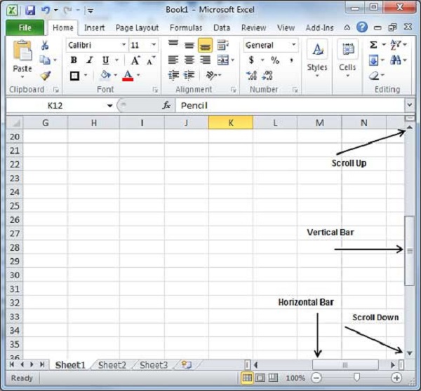
Moving with Scroll Bars
As shown in the above screen capture, there are two scroll bars: one for moving vertically within the sheet, and one for moving horizontally. Using the vertical scroll bar, you may −
-
Move upward by one line by clicking the upward-pointing scroll arrow.
-
Move downward by one line by clicking the downward-pointing scroll arrow.
-
Move one next page, using next page button (footnote).
-
Move one previous page, using previous page button (footnote).
-
Use Browse Object button to move through the sheet, going from one chosen object to the next.
Moving with Keyboard
The following keyboard commands, used for moving around your sheet, also move the insertion point −
| Keystroke | Where the Insertion Point Moves |
|---|---|
 |
Forward one box |
 |
Back one box |
 |
Up one box |
 |
Down one box |
| PageUp | To the previous screen |
| PageDown | To the next screen |
| Home | To the beginning of the current screen |
| End | To the end of the current screen |
You can move box by box or sheet by sheet. Now click in any box containing data in the sheet. You would have to hold down the Ctrl key while pressing an arrow key, which moves the insertion point as described here −
| Key Combination | Where the Insertion Point Moves |
|---|---|
| Ctrl + |
To the last box containing data of the current row. |
| Ctrl + |
To the first box containing data of the current row. |
| Ctrl + |
To the first box containing data of the current column. |
| Ctrl + |
To the last box containing data of the current column. |
| Ctrl + PageUp | To the sheet in the left of the current sheet. |
| Ctrl + PageDown | To the sheet in the right of the current sheet. |
| Ctrl + Home | To the beginning of the sheet. |
| Ctrl + End | To the end of the sheet. |
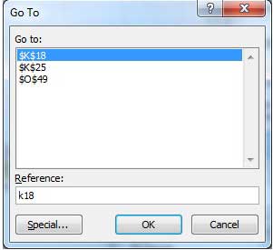
Moving with Go To Command
Press F5 key to use Go To command, which will display a dialogue box where you will find various options to reach to a particular box.
Normally, we use row and column number, for example K5 and finally press Go To button.
Save Workbook in Excel 2010
Saving New Sheet
Once you are done with typing in your new excel sheet, it is time to save your sheet/workbook to avoid losing work you have done on an Excel sheet. Following are the steps to save an edited excel sheet −
Step 1 − Click the File tab and select Save As option.
Step 2 − Select a folder where you would like to save the sheet, Enter file name, which you want to give to your sheet and Select a Save as type, by default it is .xlsx format.
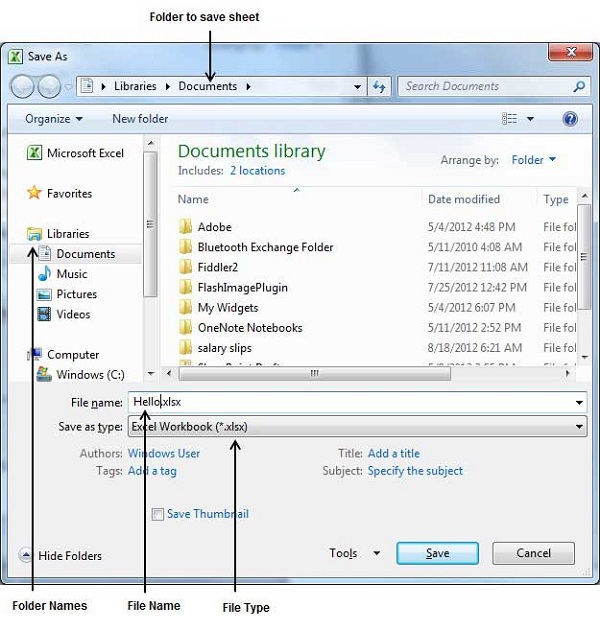
Step 3 − Finally, click on Save button and your sheet will be saved with the entered name in the selected folder.
Saving New Changes
There may be a situation when you open an existing sheet and edit it partially or completely, or even you would like to save the changes in between editing of the sheet. If you want to save this sheet with the same name, then you can use either of the following simple options −
-
Just press Ctrl + S keys to save the changes.
-
Optionally, you can click on the floppy icon available at the top left corner and just above the File tab. This option will also save the changes.
-
You can also use third method to save the changes, which is the Save option available just above the Save As option as shown in the above screen capture.
If your sheet is new and it was never saved so far, then with either of the three options, word would display you a dialogue box to let you select a folder, and enter sheet name as explained in case of saving new sheet.
Create Worksheet in Excel 2010
Creating New Worksheet
Three new blank sheets always open when you start Microsoft Excel. Below steps explain you how to create a new worksheet if you want to start another new worksheet while you are working on a worksheet, or you closed an already opened worksheet and want to start a new worksheet.
Step 1 − Right Click the Sheet Name and select Insert option.
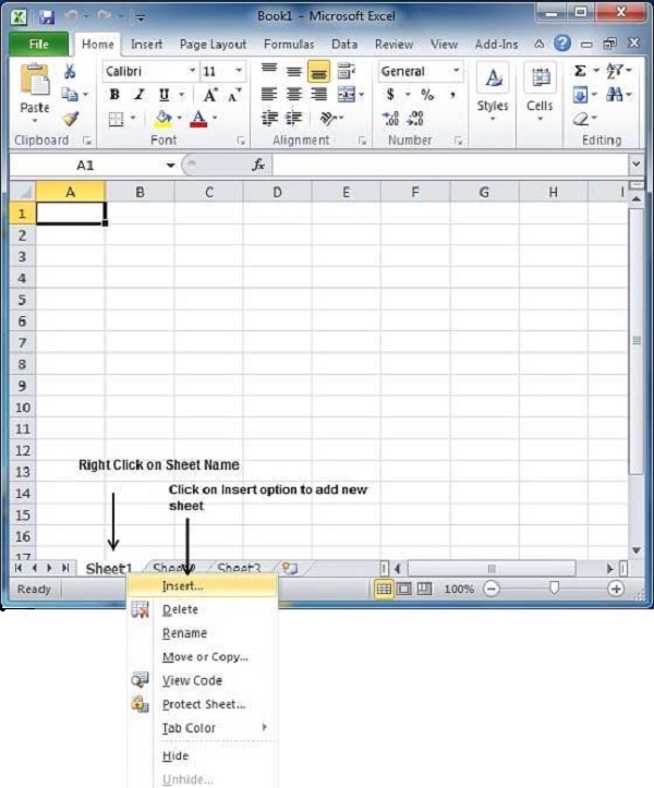
Step 2 − Now you’ll see the Insert dialog with select Worksheet option as selected from the general tab. Click the Ok button.
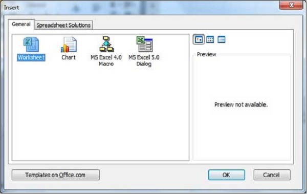
Now you should have your blank sheet as shown below ready to start typing your text.
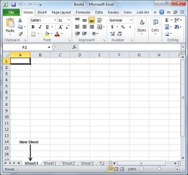
You can use a short cut to create a blank sheet anytime. Try using the Shift+F11 keys and you will see a new blank sheet similar to the above sheet is opened.
Copy Worksheet in Excel 2010
Copy Worksheet
First of all, let us create some sample text before we proceed. Open a new excel sheet and type any data. We’ve shown a sample data in the screenshot.
| OrderDate | Region | Rep | Item | Units | Unit Cost | Total |
|---|---|---|---|---|---|---|
| 1/6/2010 | East | Jones | Pencil | 95 | 1.99 | 189.05 |
| 1/23/2010 | Central | Kivell | Binder | 50 | 19.99 | 999.5 |
| 2/9/2010 | Central | Jardine | Pencil | 36 | 4.99 | 179.64 |
| 2/26/2010 | Central | Gill | Pen | 27 | 19.99 | 539.73 |
| 3/15/2010 | West | Sorvino | Pencil | 56 | 2.99 | 167.44 |
| 4/1/2010 | East | Jones | Binder | 60 | 4.99 | 299.4 |
| 4/18/2010 | Central | Andrews | Pencil | 75 | 1.99 | 149.25 |
| 5/5/2010 | Central | Jardine | Pencil | 90 | 4.99 | 449.1 |
| 5/22/2010 | West | Thompson | Pencil | 32 | 1.99 | 63.68 |
| 6/8/2010 | East | Jones | Binder | 60 | 8.99 | 539.4 |
| 6/25/2010 | Central | Morgan | Pencil | 90 | 4.99 | 449.1 |
| 7/12/2010 | East | Howard | Binder | 29 | 1.99 | 57.71 |
| 7/29/2010 | East | Parent | Binder | 81 | 19.99 | 1,619.19 |
| 8/15/2010 | East | Jones | Pencil | 35 | 4.99 | 174.65 |
Here are the steps to copy an entire worksheet.
Step 1 − Right Click the Sheet Name and select the Move or Copy option.
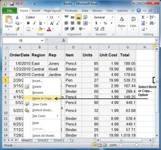
Step 2 − Now you’ll see the Move or Copy dialog with select Worksheet option as selected from the general tab. Click the Ok button.
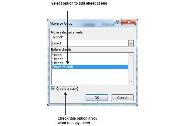
Select Create a Copy Checkbox to create a copy of the current sheet and Before sheet option as (move to end) so that new sheet gets created at the end.
Press the Ok Button.
Now you should have your copied sheet as shown below.
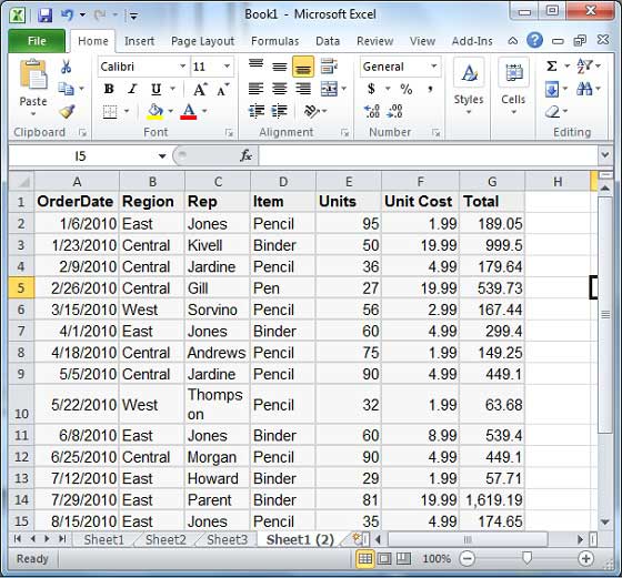
You can rename the sheet by double clicking on it. On double click, the sheet name becomes editable. Enter any name say Sheet5 and press Tab or Enter Key.
Hiding Worksheet in Excel 2010
Hiding Worksheet
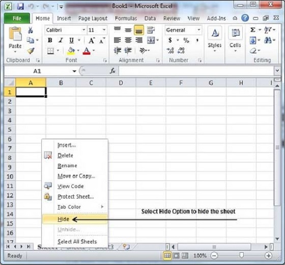
Here is the step to hide a worksheet.
Step − Right Click the Sheet Name and select the Hide option. Sheet will get hidden.
Unhiding Worksheet
Here are the steps to unhide a worksheet.
Step 1 − Right Click on any Sheet Name and select the Unhide… option.
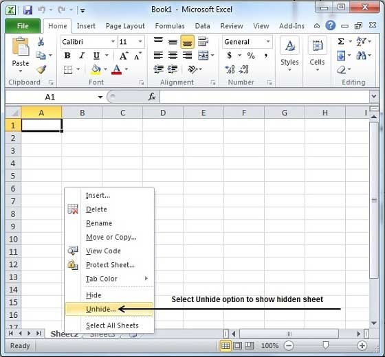
Step 2 − Select Sheet Name to unhide in Unhide dialog to unhide the sheet.
Press the Ok Button.
Now you will have your hidden sheet back.
Delete Worksheet in Excel 2010
Delete Worksheet
Here is the step to delete a worksheet.
Step − Right Click the Sheet Name and select the Delete option.
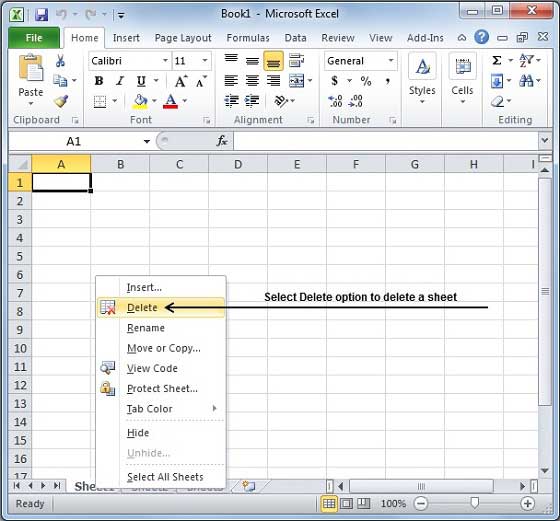
Sheet will get deleted if it is empty, otherwise you’ll see a confirmation message.
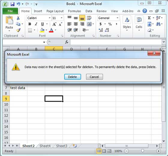
Press the Delete Button.
Now your worksheet will get deleted.
Close Workbook in Excel 2010
Close Workbook
Here are the steps to close a workbook.
Step 1 − Click the Close Button as shown below.
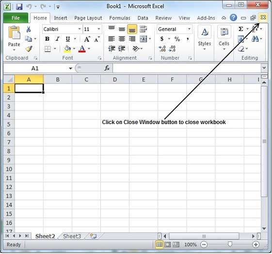
You’ll see a confirmation message to save the workbook.
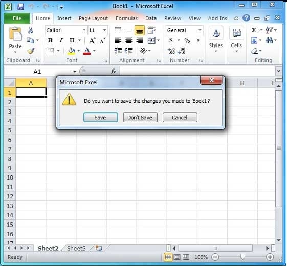
Step 2 − Press the Save Button to save the workbook as we did in MS Excel — Save Workbook chapter.
Now your worksheet will get closed.
Open Workbook in Excel 2010
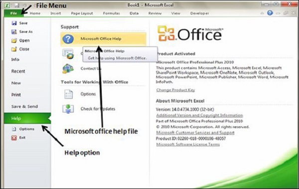
Let us see how to open workbook from excel in the below mentioned steps.
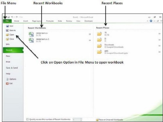
Step 1 − Click the File Menu as shown below. You can see the Open option in File Menu.
There are two more columns Recent workbooks and Recent places, where you can see the recently opened workbooks and the recent places from where workbooks are opened.
Step 2 − Clicking the Open Option will open the browse dialog as shown below. Browse the directory and find the file you need to open.
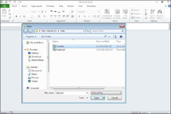
Step 3 − Once you select the workbook your workbook will be opened as below −

Context Help in Excel 2010
MS Excel provides context sensitive help on mouse over. To see context sensitive help for a particular Menu option, hover the mouse over the option for some time. Then you can see the context sensitive Help as shown below.
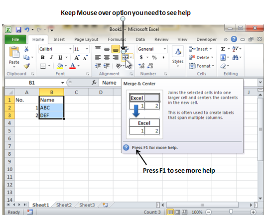
Getting More Help
For getting more help with MS Excel from Microsoft you can press F1 or by File → Help → Support → Microsoft Office Help.
Insert Data in Excel 2010
In MS Excel, there are 1048576*16384 cells. MS Excel cell can have Text, Numeric value or formulas. An MS Excel cell can have maximum of 32000 characters.
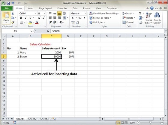
Inserting Data
For inserting data in MS Excel, just activate the cell type text or number and press enter or Navigation keys.
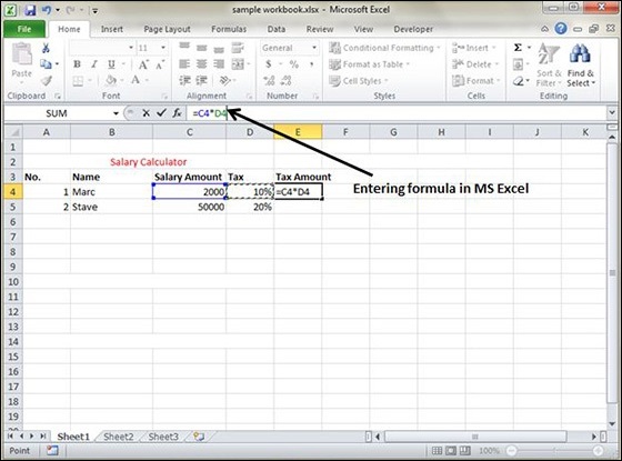
Inserting Formula
For inserting formula in MS Excel go to the formula bar, enter the formula and then press enter or navigation key. See the screen-shot below to understand it.
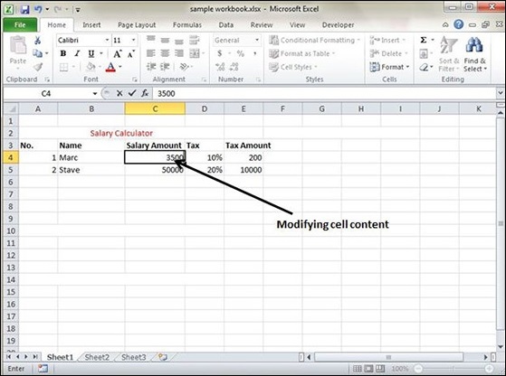
Modifying Cell Content
For modifying the cell content just activate the cell, enter a new value and then press enter or navigation key to see the changes. See the screen-shot below to understand it.
Select Data in Excel 2010
MS Excel provides various ways of selecting data in the sheet. Let us see those ways.
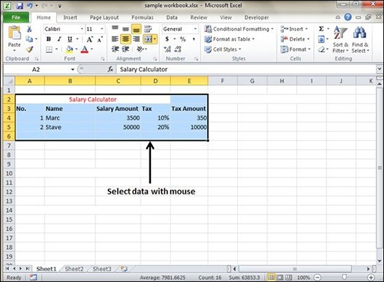
Select with Mouse
Drag the mouse over the data you want to select. It will select those cells as shown below.
Select with Special
If you want to select specific region, select any cell in that region. Pressing F5 will show the below dialogue box.
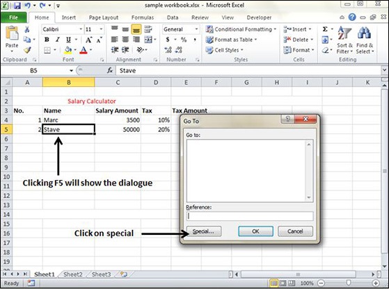
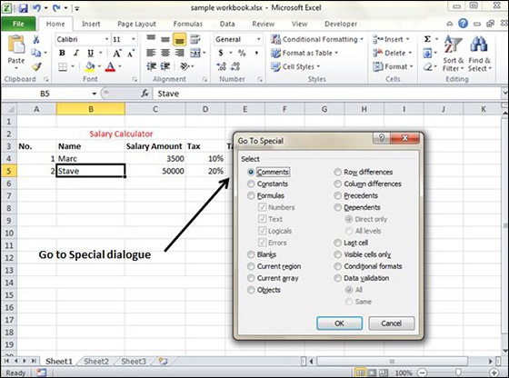
Click on Special button to see the below dialogue box. Select current region from the radio buttons. Click on ok to see the current region selected.
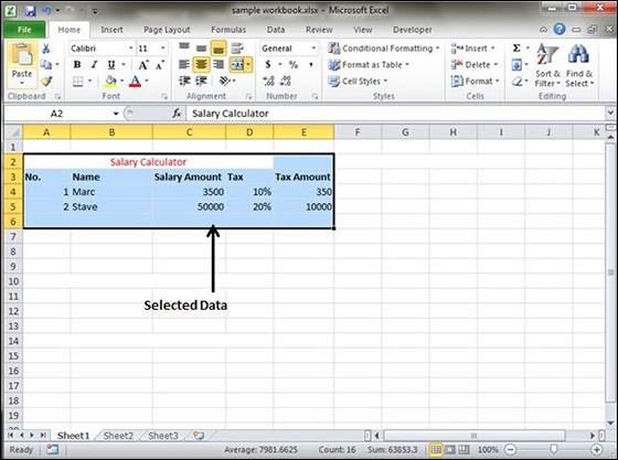
As you can see in the below screen, the data is selected for the current region.
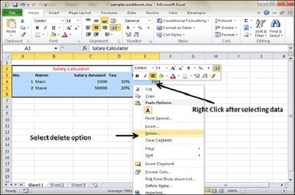
Delete Data in Excel 2010
MS Excel provides various ways of deleting data in the sheet. Let us see those ways.
Delete with Mouse
Select the data you want to delete. Right Click on the sheet. Select the delete option, to delete the data.
Delete with Delete Key
Select the data you want to delete. Press on the Delete Button from the keyboard, it will delete the data.
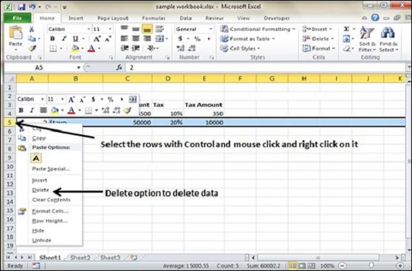
Selective Delete for Rows
Select the rows, which you want to delete with Mouse click + Control Key. Then right click to show the various options. Select the Delete option to delete the selected rows.
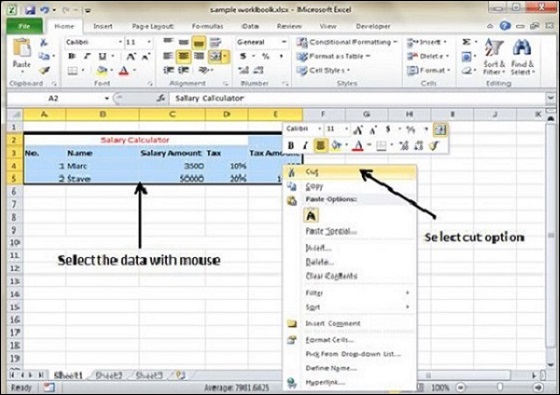
Move Data in Excel 2010
Let us see how we can Move Data with MS Excel.
Step 1 − Select the data you want to Move. Right Click and Select the cut option.
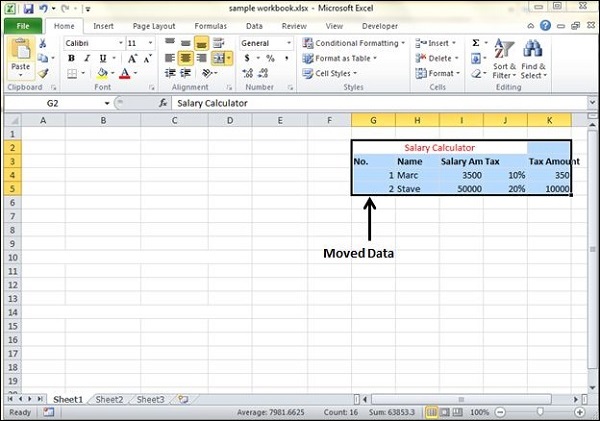
Step 2 − Select the first cell where you want to move the data. Right click on it and paste the data. You can see the data is moved now.
Rows & Columns in Excel 2010
Row and Column Basics
MS Excel is in tabular format consisting of rows and columns.
-
Row runs horizontally while Column runs vertically.
-
Each row is identified by row number, which runs vertically at the left side of the sheet.
-
Each column is identified by column header, which runs horizontally at the top of the sheet.
For MS Excel 2010, Row numbers ranges from 1 to 1048576; in total 1048576 rows, and Columns ranges from A to XFD; in total 16384 columns.
Navigation with Rows and Columns
Let us see how to move to the last row or the last column.
-
You can go to the last row by clicking Control + Down Navigation arrow.
-
You can go to the last column by clicking Control + Right Navigation arrow.
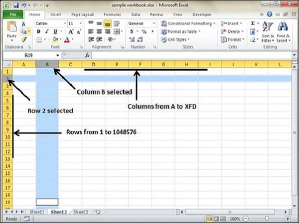
Cell Introduction
The intersection of rows and columns is called cell.
Cell is identified with Combination of column header and row number.
For example − A1, A2.
Copy & Paste in Excel 2010
MS Excel provides copy paste option in different ways. The simplest method of copy paste is as below.
Copy Paste
-
To copy and paste, just select the cells you want to copy. Choose copy option after right click or press Control + C.
-
Select the cell where you need to paste this copied content. Right click and select paste option or press Control + V.
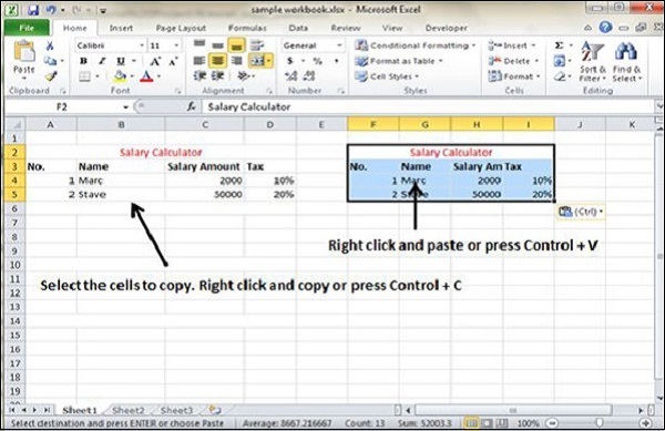
In this case, MS Excel will copy everything such as values, formulas, Formats, Comments and validation. MS Excel will overwrite the content with paste. If you want to undo this, press Control + Z from the keyboard.
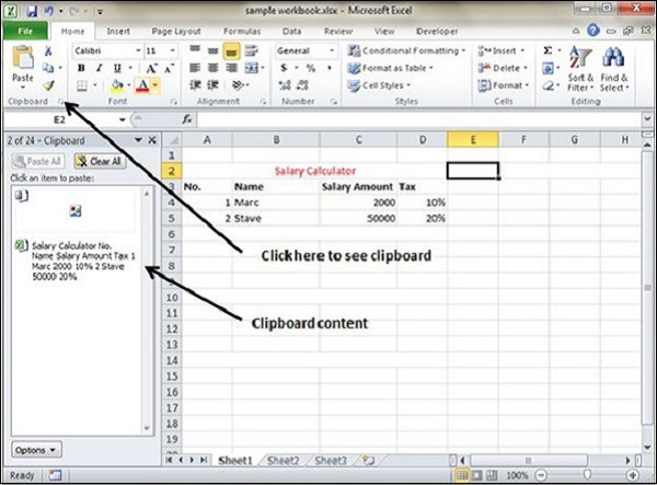
Copy Paste using Office Clipboard
When you copy data in MS Excel, it puts the copied content in Windows and Office Clipboard. You can view the clipboard content by Home → Clipboard. View the clipboard content. Select the cell where you need to paste. Click on paste, to paste the content.
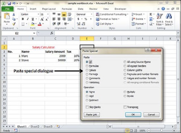
Copy Paste in Special way
You may not want to copy everything in some cases. For example, you want to copy only Values or you want to copy only the formatting of cells. Select the paste special option as shown below.
Below are the various options available in paste special.
-
All − Pastes the cell’s contents, formats, and data validation from the Windows Clipboard.
-
Formulas − Pastes formulas, but not formatting.
-
Values − Pastes only values not the formulas.
-
Formats − Pastes only the formatting of the source range.
-
Comments − Pastes the comments with the respective cells.
-
Validation − Pastes validation applied in the cells.
-
All using source theme − Pastes formulas, and all formatting.
-
All except borders − Pastes everything except borders that appear in the source range.
-
Column Width − Pastes formulas, and also duplicates the column width of the copied cells.
-
Formulas & Number Formats − Pastes formulas and number formatting only.
-
Values & Number Formats − Pastes the results of formulas, plus the number.
-
Merge Conditional Formatting − This icon is displayed only when the copied cells contain conditional formatting. When clicked, it merges the copied conditional formatting with any conditional formatting in the destination range.
-
Transpose − Changes the orientation of the copied range. Rows become columns, and columns become rows. Any formulas in the copied range are adjusted so that they work properly when transposed.
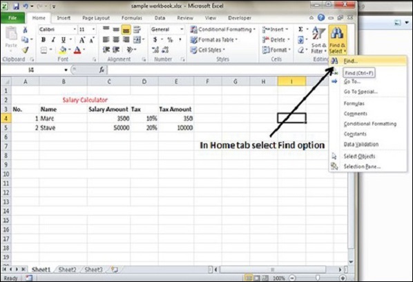
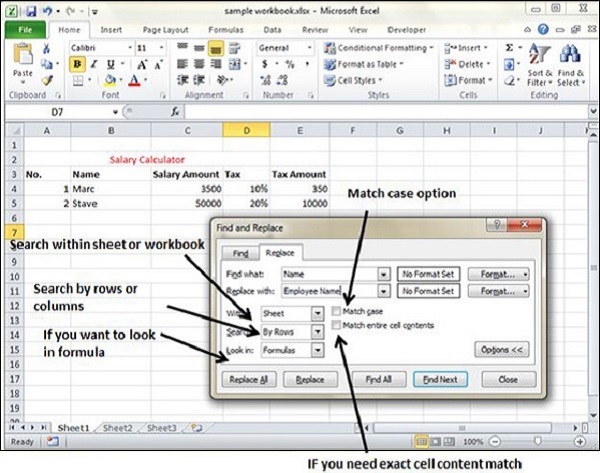
Find & Replace in Excel 2010
MS Excel provides Find & Replace option for finding text within the sheet.
Find and Replace Dialogue
Let us see how to access the Find & Replace Dialogue.
To access the Find & Replace, Choose Home → Find & Select → Find or press Control + F Key. See the image below.
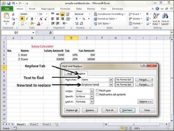
You can see the Find and Replace dialogue as below.
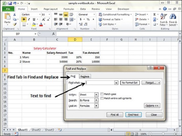
You can replace the found text with the new text in the Replace tab.
Exploring Options
Now, let us see the various options available under the Find dialogue.
-
Within − Specifying the search should be in Sheet or workbook.
-
Search By − Specifying the internal search method by rows or by columns.
-
Look In − If you want to find text in formula as well, then select this option.
-
Match Case − If you want to match the case like lower case or upper case of words, then check this option.
-
Match Entire Cell Content − If you want the exact match of the word with cell, then check this option.
Spell Check in Excel 2010
MS Excel provides a feature of Word Processing program called Spelling check. We can get rid of the spelling mistakes with the help of spelling check feature.
Spell Check Basis
Let us see how to access the spell check.
-
To access the spell checker, Choose Review ➪ Spelling or press F7.
-
To check the spelling in just a particular range, select the range before you activate the spell checker.
-
If the spell checker finds any words it does not recognize as correct, it displays the Spelling dialogue with suggested options.
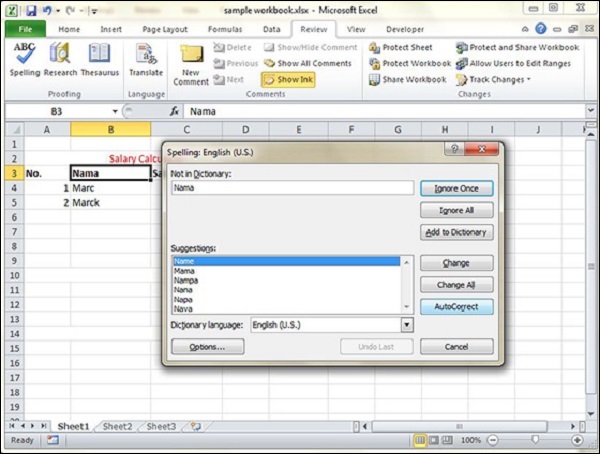
Exploring Options
Let us see the various options available in spell check dialogue.
-
Ignore Once − Ignores the word and continues the spell check.
-
Ignore All − Ignores the word and all subsequent occurrences of it.
-
Add to Dictionary − Adds the word to the dictionary.
-
Change − Changes the word to the selected word in the Suggestions list.
-
Change All − Changes the word to the selected word in the Suggestions list and changes all subsequent occurrences of it without asking.
-
AutoCorrect − Adds the misspelled word and its correct spelling (which you select from the list) to the AutoCorrect list.
Zoom In/Out in Excel 2010
Zoom Slider
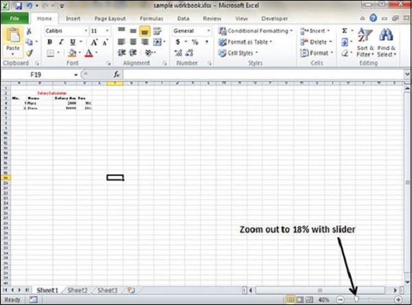
By default, everything on screen is displayed at 100% in MS Excel. You can change the zoom percentage from 10% (tiny) to 400% (huge). Zooming doesn’t change the font size, so it has no effect on the printed output.
You can view the zoom slider at the right bottom of the workbook as shown below.
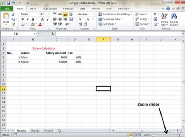
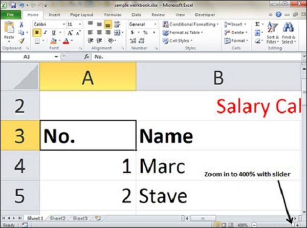
Zoom In
You can zoom in the workbook by moving the slider to the right. It will change the only view of the workbook. You can have maximum of 400% zoom in. See the below screen-shot.
Zoom Out
You can zoom out the workbook by moving the slider to the left. It will change the only view of the workbook. You can have maximum of 10% zoom in. See the below screen-shot.
Special Symbols in Excel 2010
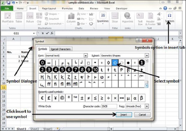
If you want to insert some symbols or special characters that are not found on the keyboard in that case you need to use the Symbols option.
Using Symbols
Go to Insert » Symbols » Symbol to view available symbols. You can see many symbols available there like Pi, alpha, beta, etc.
Select the symbol you want to add and click insert to use the symbol.
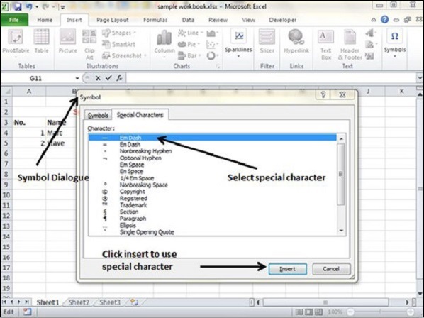
Using Special Characters
Go to Insert » Symbols » Special Characters to view the available special characters. You can see many special characters available there like Copyright, Registered etc.
Select the special character you want to add and click insert, to use the special character.
Insert Comments in Excel 2010
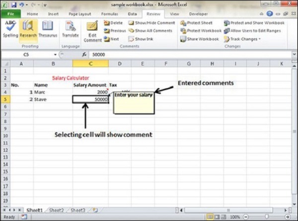
Adding Comment to Cell
Adding comment to cell helps in understanding the purpose of cell, what input it should have, etc. It helps in proper documentation.
To add comment to a cell, select the cell and perform any of the actions mentioned below.
- Choose Review » Comments » New Comment.
- Right-click the cell and choose Insert Comment from available options.
- Press Shift+F2.
Initially, a comment consists of Computer’s user name. You have to modify it with text for the cell comment.
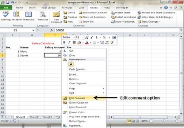
Modifying Comment
You can modify the comment you have entered before as mentioned below.
- Select the cell on which the comment appears.
- Right-click the cell and choose the Edit Comment from the available options.
- Modify the comment.
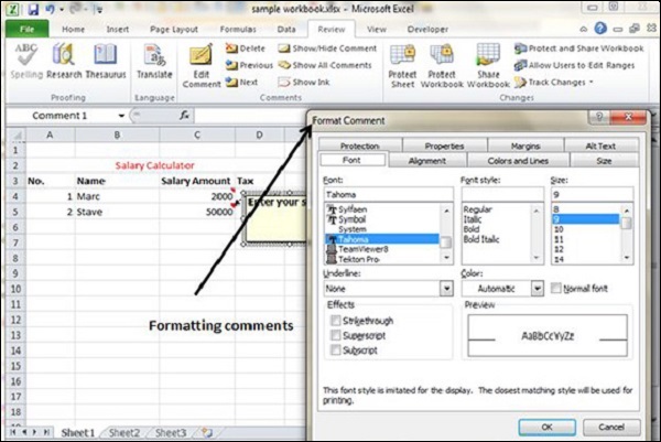
Formatting Comment
Various formatting options are available for comments. For formatting a comment, Right click on cell » Edit comment » Select comment » Right click on it » Format comment. With formatting of comment you can change the color, font, size, etc of the comment.
Add Text Box in Excel 2010
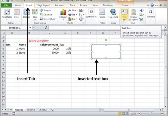
Text Boxes
Text boxes are special graphic objects that combine the text with a rectangular graphic object. Text boxes and cell comments are similar in displaying the text in rectangular box. But text boxes are always visible, while cell comments become visible after selecting the cell.
Adding Text Boxes
To add a text box, perform the below actions.
- Choose Insert » Text Box » choose text box or draw it.
Initially, the comment consists of Computer’s user name. You have to modify it with text for the cell comment.
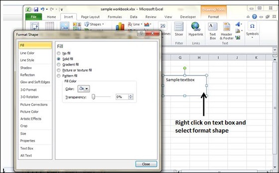
Formatting Text Box
After you have added the text box, you can format it by changing the font, font size, font style, and alignment, etc. Let us see some of the important options of formatting a text box.
-
Fill − Specifies the filling of text box like No fill, solid fill. Also specifying the transparency of text box fill.
-
Line Colour − Specifies the line colour and transparency of the line.
-
Line Style − Specifies the line style and width.
-
Size − Specifies the size of the text box.
-
Properties − Specifies some properties of the text box.
-
Text Box − Specifies text box layout, Auto-fit option and internal margins.
Undo Changes in Excel 2010
Undo Changes
You can reverse almost every action in Excel by using the Undo command. We can undo changes in following two ways.
- From the Quick access tool-bar » Click Undo.
- Press Control + Z.
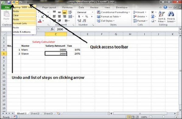
You can reverse the effects of the past 100 actions that you performed by executing Undo more than once. If you click the arrow on the right side of the Undo button, you see a list of the actions that you can reverse. Click an item in that list to undo that action and all the subsequent actions you performed.
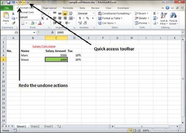
Redo Changes
You can again reverse back the action done with undo in Excel by using the Redo command. We can redo changes in following two ways.
- From the Quick access tool-bar » Click Redo.
- Press Control + Y.
Setting Cell Type in Excel 2010
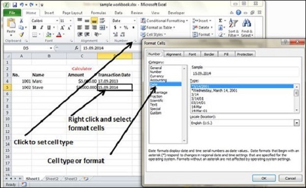
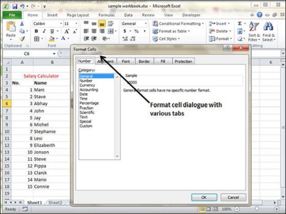
Formatting Cell
MS Excel Cell can hold different types of data like Numbers, Currency, Dates, etc. You can set the cell type in various ways as shown below −
- Right Click on the cell » Format cells » Number.
- Click on the Ribbon from the ribbon.
Various Cell Formats
Below are the various cell formats.
-
General − This is the default cell format of Cell.
-
Number − This displays cell as number with separator.
-
Currency − This displays cell as currency i.e. with currency sign.
-
Accounting − Similar to Currency, used for accounting purpose.
-
Date − Various date formats are available under this like 17-09-2013, 17th-Sep-2013, etc.
-
Time − Various Time formats are available under this, like 1.30PM, 13.30, etc.
-
Percentage − This displays cell as percentage with decimal places like 50.00%.
-
Fraction − This displays cell as fraction like 1/4, 1/2 etc.
-
Scientific − This displays cell as exponential like 5.6E+01.
-
Text − This displays cell as normal text.
-
Special − Special formats of cell like Zip code, Phone Number.
-
Custom − You can use custom format by using this.
Setting Fonts in Excel 2010
You can assign any of the fonts that is installed for your printer to cells in a worksheet.
Setting Font from Home
You can set the font of the selected text from Home » Font group » select the font.
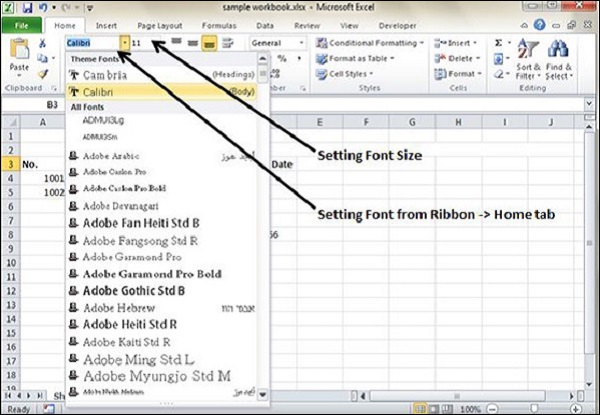
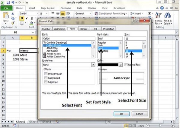
Setting Font From Format Cell Dialogue
- Right click on cell » Format cells » Font Tab
- Press Control + 1 or Shift + Control + F
Text Decoration in Excel 2010
You can change the text decoration of the cell to change its look and feel.
Text Decoration
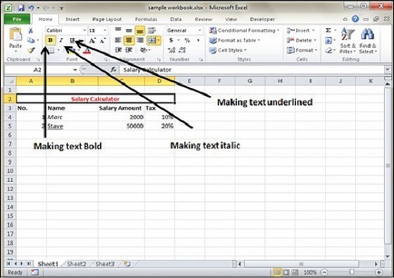
Various options are available in Home tab of the ribbon as mentioned below.
-
Bold − It makes the text in bold by choosing Home » Font Group » Click B or Press Control + B.
-
Italic − It makes the text italic by choosing Home » Font Group » Click I or Press Control + I.
-
Underline − It makes the text to be underlined by choosing Home » Font Group » Click U or Press Control + U.
-
Double Underline − It makes the text highlighted as double underlined by choose Home » Font Group » Click arrow near U » Select Double Underline.
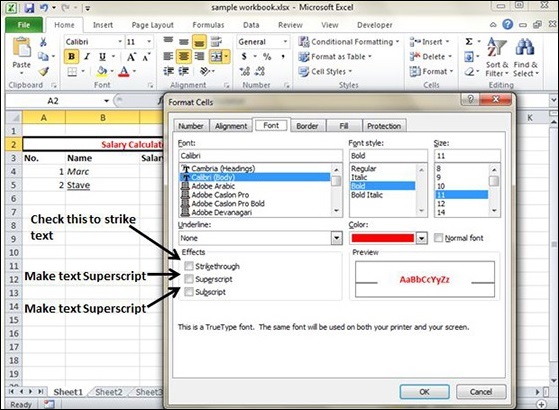
More Text Decoration Options
There are more options available for text decoration in Formatting cells » Font Tab »Effects cells as mentioned below.
-
Strike-through − It strikes the text in the center vertically.
-
Super Script − It makes the content to appear as a super script.
-
Sub Script − It makes content to appear as a sub script.
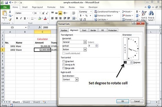
Rotate Cells in Excel 2010
You can rotate the cell by any degree to change the orientation of the cell.
Rotating Cell from Home Tab
Click on the orientation in the Home tab. Choose options available like Angle CounterClockwise, Angle Clockwise, etc.
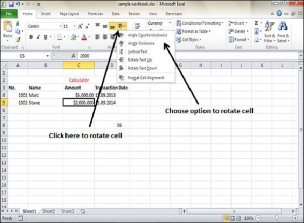
Rotating Cell from Formatting Cell
Right Click on the cell. Choose Format cells » Alignment » Set the degree for rotation.
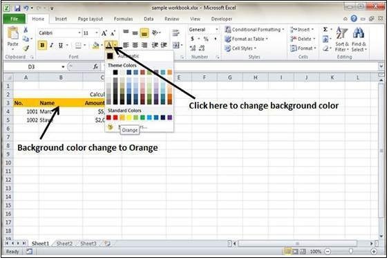
Setting Colors in Excel 2010
You can change the background color of the cell or text color.
Changing Background Color
By default the background color of the cell is white in MS Excel. You can change it as per your need from Home tab » Font group » Background color.
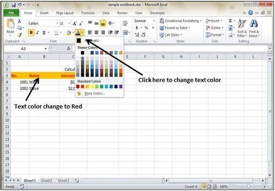
Changing Foreground Color
By default, the foreground or text color is black in MS Excel. You can change it as per your need from Home tab » Font group » Foreground color.
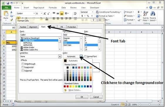
Also you can change the foreground color by selecting the cell Right click » Format cells » Font Tab » Color.
Text Alignments in Excel 2010
If you don’t like the default alignment of the cell, you can make changes in the alignment of the cell. Below are the various ways of doing it.
Change Alignment from Home Tab
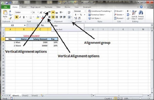
You can change the Horizontal and vertical alignment of the cell. By default, Excel aligns numbers to the right and text to the left. Click on the available option in the Alignment group in Home tab to change alignment.
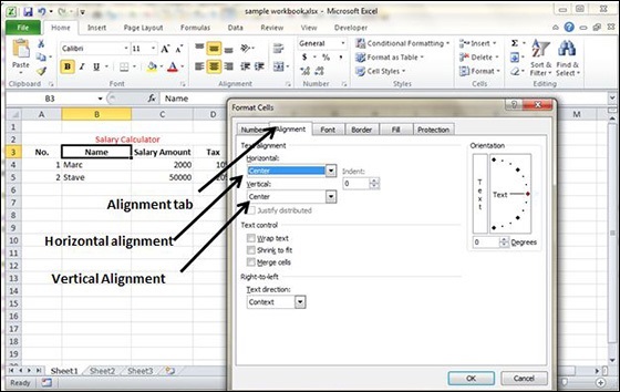
Change Alignment from Format Cells
Right click on the cell and choose format cell. In format cells dialogue, choose Alignment Tab. Select the available options from the Vertical alignment and Horizontal alignment options.
Exploring Alignment Options
1. Horizontal Alignment − You can set horizontal alignment to Left, Centre, Right, etc.
-
Left − Aligns the cell contents to the left side of the cell.
-
Center − Centers the cell contents in the cell.
-
Right − Aligns the cell contents to the right side of the cell.
-
Fill − Repeats the contents of the cell until the cell’s width is filled.
-
Justify − Justifies the text to the left and right of the cell. This option is applicable only if the cell is formatted as wrapped text and uses more than one line.
2. Vertical Alignment − You can set Vertical alignment to top, Middle, bottom, etc.
-
Top Aligns the cell contents to the top of the cell.
-
Center Centers the cell contents vertically in the cell.
-
Bottom Aligns the cell contents to the bottom of the cell.
-
Justify Justifies the text vertically in the cell; this option is applicable only if the cell is formatted as wrapped text and uses more than one line.
Merge & Wrap in Excel 2010
Merge Cells
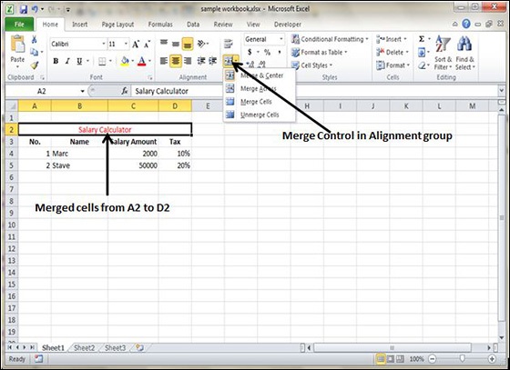
MS Excel enables you to merge two or more cells. When you merge cells, you don’t combine the contents of the cells. Rather, you combine a group of cells into a single cell that occupies the same space.
You can merge cells by various ways as mentioned below.
-
Choose Merge & Center control on the Ribbon, which is simpler. To merge cells, select the cells that you want to merge and then click the Merge & Center button.
-
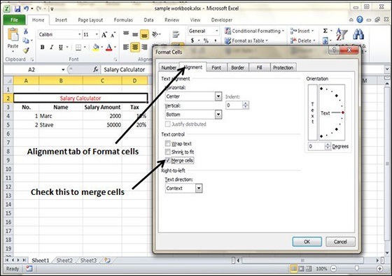
Choose Alignment tab of the Format Cells dialogue box to merge the cells.
Additional Options
The Home » Alignment group » Merge & Center control contains a drop-down list with these additional options −
-
Merge Across − When a multi-row range is selected, this command creates multiple merged cells — one for each row.
-
Merge Cells − Merges the selected cells without applying the Center attribute.
-
Unmerge Cells − Unmerges the selected cells.
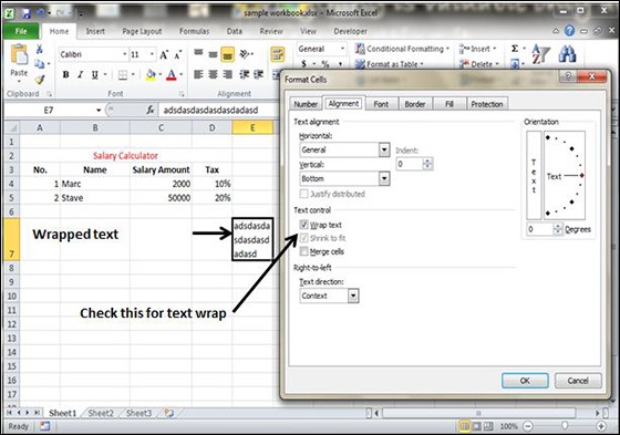
Wrap Text and Shrink to Fit
If the text is too wide to fit the column width but don’t want that text to spill over into adjacent cells, you can use either the Wrap Text option or the Shrink to Fit option to accommodate that text.
Borders and Shades in Excel 2010
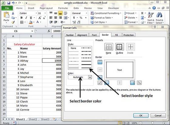
Apply Borders
MS Excel enables you to apply borders to the cells. For applying border, select the range of cells Right Click » Format cells » Border Tab » Select the Border Style.
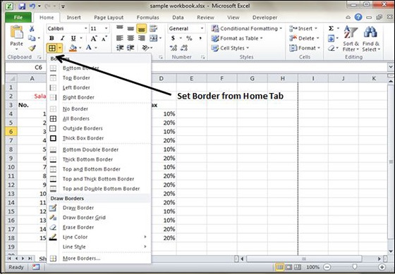
Then you can apply border by Home Tab » Font group »Apply Borders.
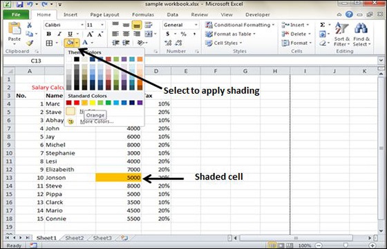
Apply Shading
You can add shading to the cell from the Home tab » Font Group » Select the Color.
Apply Formatting in Excel 2010
Formatting Cells
In MS Excel, you can apply formatting to the cell or range of cells by Right Click » Format cells » Select the tab. Various tabs are available as shown below
Alternative to Placing Background
-
Number − You can set the Format of the cell depending on the cell content. Find tutorial on this at MS Excel — Setting Cell Type.
-
Alignment − You can set the alignment of text on this tab. Find tutorial on this at MS Excel — Text Alignments.
-
Font − You can set the Font of text on this tab.Find tutorial on this at MS Excel — Setting Fonts.
-
Border − You can set border of cell with this tab.Find tutorial on this at MS Excel — Borders and Shades.
-
Fill − You can set fill of cell with this tab. Find tutorial on this at MS Excel — Borders and Shades.
-
Protection − You can set cell protection option with this tab.
Sheet Options in Excel 2010
Sheet Options
MS Excel provides various sheet options for printing purpose like generally cell gridlines aren’t printed. If you want your printout to include the gridlines, Choose Page Layout » Sheet Options group » Gridlines » Check Print.
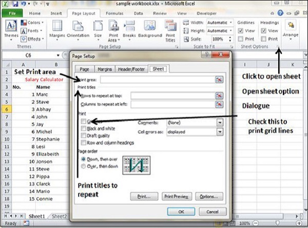
Options in Sheet Options Dialogue
-
Print Area − You can set the print area with this option.
-
Print Titles − You can set titles to appear at the top for rows and at the left for columns.
-
Print −
-
Gridlines − Gridlines to appear while printing worksheet.
-
Black & White − Select this check box to have your color printer print the chart in black and white.
-
Draft quality − Select this check box to print the chart using your printer’s draft-quality setting.
-
Rows & Column Heading − Select this check box to have rows and column heading to print.
-
-
Page Order −
-
Down, then Over − It prints the down pages first and then the right pages.
-
Over, then Down − It prints right pages first and then comes to print the down pages.
-
Adjust Margins in Excel 2010
Margins
Margins are the unprinted areas along the sides, top, and bottom of a printed page. All printed pages in MS Excel have the same margins. You can’t specify different margins for different pages.
You can set margins by various ways as explained below.
-
Choose Page Layout » Page Setup » Margins drop-down list, you can select Normal, Wide, Narrow, or the custom Setting.
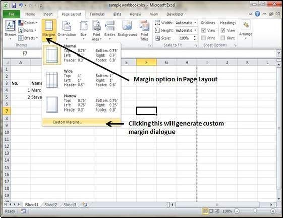
-
These options are also available when you choose File » Print.
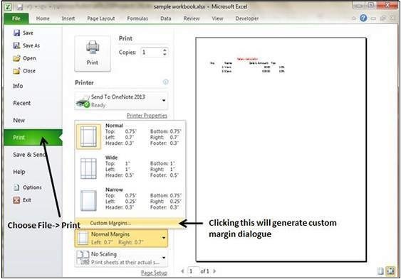
If none of these settings does the job, choose Custom Margins to display the Margins tab of the Page Setup dialog box, as shown below.
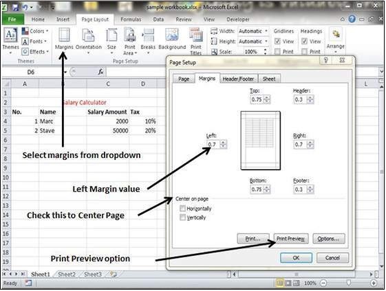
Center on Page
By default, Excel aligns the printed page at the top and left margins. If you want the output to be centered vertically or horizontally, select the appropriate check box in the Center on Page section of the Margins tab as shown in the above screenshot.
Page Orientation in Excel 2010
Page Orientation
Page orientation refers to how output is printed on the page. If you change the orientation, the onscreen page breaks adjust automatically to accommodate the new paper orientation.
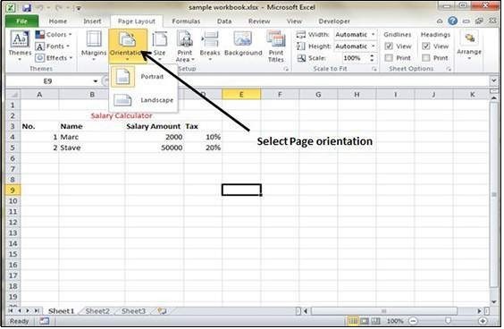
Types of Page Orientation
-
Portrait − Portrait to print tall pages (the default).
-
Landscape − Landscape to print wide pages. Landscape orientation is useful when you have a wide range that doesn’t fit on a vertically oriented page.
Changing Page Orientation
-
Choose Page Layout » Page Setup » Orientation » Portrait or Landscape.
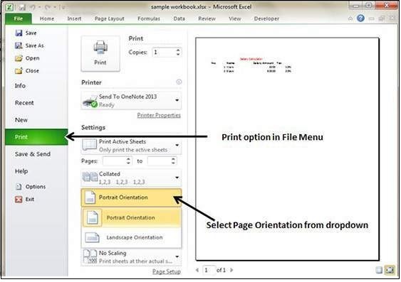
- Choose File » Print.
Header and Footer in Excel 2010
Header and Footer
A header is the information that appears at the top of each printed page and a footer is the information that appears at the bottom of each printed page. By default, new workbooks do not have headers or footers.
Adding Header and Footer
- Choose Page Setup dialog box » Header or Footer tab.
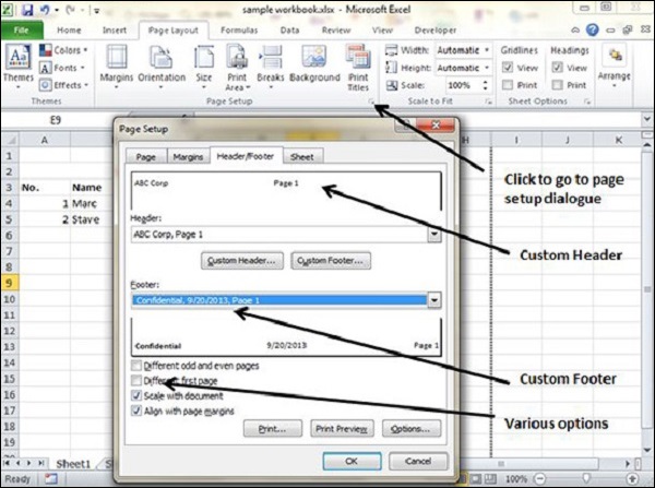
You can choose the predefined header and footer or create your custom ones.
-
&[Page] − Displays the page number.
-
&[Pages] − Displays the total number of pages to be printed.
-
&[Date] − Displays the current date.
-
&[Time] − Displays the current time.
-
&[Path]&[File] − Displays the workbook’s complete path and filename.
-
&[File] − Displays the workbook name.
-
&[Tab] − Displays the sheet’s name.
Other Header and Footer Options
When a header or footer is selected in Page Layout view, the Header & Footer » Design » Options group contains controls that let you specify other options −
-
Different First Page − Check this to specify a different header or footer for the first printed page.
-
Different Odd & Even Pages − Check this to specify a different header or footer for odd and even pages.
-
Scale with Document − If checked, the font size in the header and footer will be sized. Accordingly if the document is scaled when printed. This option is enabled, by default.
-
Align with Page Margins − If checked, the left header and footer will be aligned with the left margin, and the right header and footer will be aligned with the right margin. This option is enabled, by default.
Insert Page Break in Excel 2010
Page Breaks
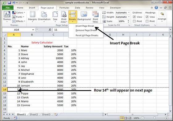
If you don’t want a row to print on a page by itself or you don’t want a table header row to be the last line on a page. MS Excel gives you precise control over page breaks.
MS Excel handles page breaks automatically, but sometimes you may want to force a page break either a vertical or a horizontal one. so that the report prints the way you want.
For example, if your worksheet consists of several distinct sections, you may want to print each section on a separate sheet of paper.
Inserting Page Breaks
Insert Horizontal Page Break − For example, if you want row 14 to be the first row of a new page, select cell A14. Then choose Page Layout » Page Setup Group » Breaks» Insert Page Break.
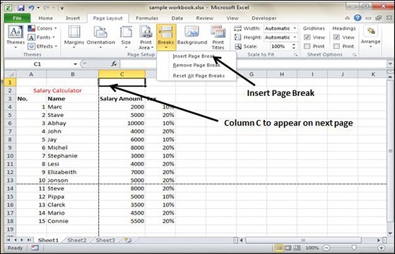
Insert vertical Page break − In this case, make sure to place the pointer in row 1. Choose Page Layout » Page Setup » Breaks » Insert Page Break to create the page break.
Removing Page Breaks
-
Remove a page break you’ve added − Move the cell pointer to the first row beneath the manual page break and then choose Page Layout » Page Setup » Breaks » Remove Page Break.
-
Remove all manual page breaks − Choose Page Layout » Page Setup » Breaks » Reset All Page Breaks.
Set Background in Excel 2010
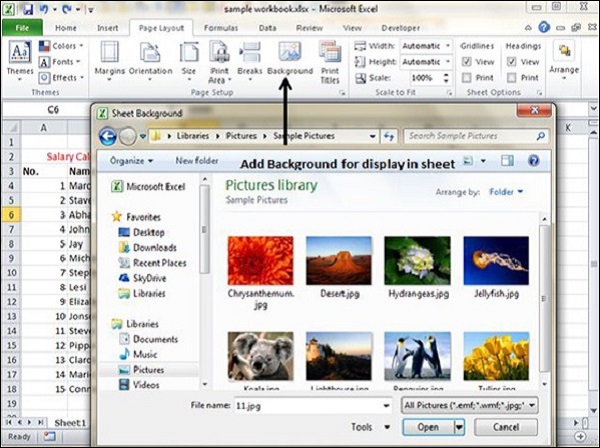
Background Image
Unfortunately, you cannot have a background image on your printouts. You may have noticed the Page Layout » Page Setup » Background command. This button displays a dialogue box that lets you select an image to display as a background. Placing this control among the other print-related commands is very misleading. Background images placed on a worksheet are never printed.
Alternative to Placing Background
-
You can insert a Shape, WordArt, or a picture on your worksheet and then adjust its transparency. Then copy the image to all printed pages.
-
You can insert an object in a page header or footer.
Freeze Panes in Excel 2010
Freezing Panes
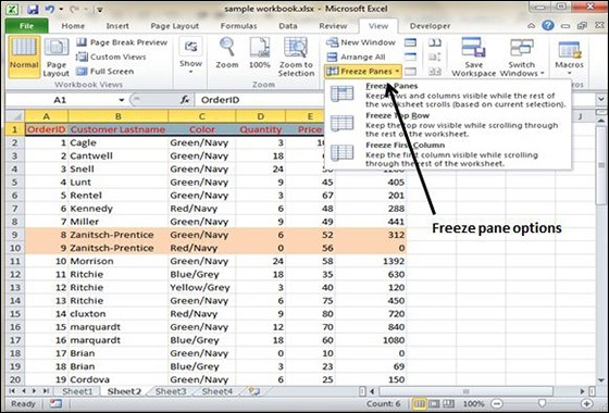
If you set up a worksheet with row or column headings, these headings will not be visible when you scroll down or to the right. MS Excel provides a handy solution to this problem with freezing panes. Freezing panes keeps the headings visible while you’re scrolling through the worksheet.
Using Freeze Panes
Follow the steps mentioned below to freeze panes.
-
Select the First row or First Column or the row Below, which you want to freeze, or Column right to area, which you want to freeze.
-
Choose View Tab » Freeze Panes.
-
Select the suitable option −
-
Freeze Panes − To freeze area of cells.
-
Freeze Top Row − To freeze first row of worksheet.
-
Freeze First Column − To freeze first Column of worksheet.
-
-
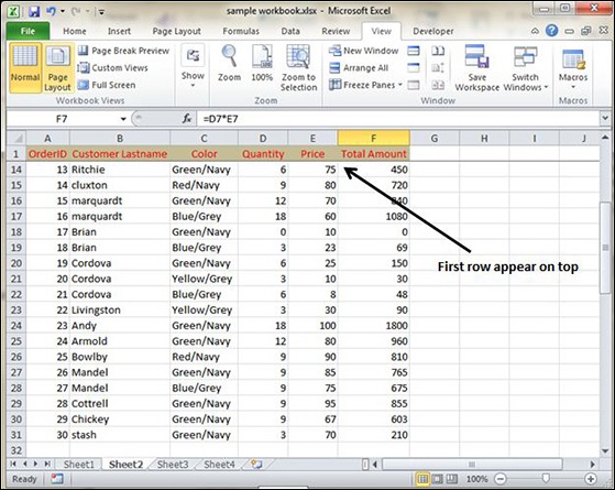
If you have selected Freeze top row you can see the first row appears at the top, after scrolling also. See the below screen-shot.
Unfreeze Panes
To unfreeze Panes, choose View Tab » Unfreeze Panes.
Conditional Format in Excel 2010
Conditional Formatting
MS Excel 2010 Conditional Formatting feature enables you to format a range of values so that the values outside certain limits, are automatically formatted.
Choose Home Tab » Style group » Conditional Formatting dropdown.
Various Conditional Formatting Options
-
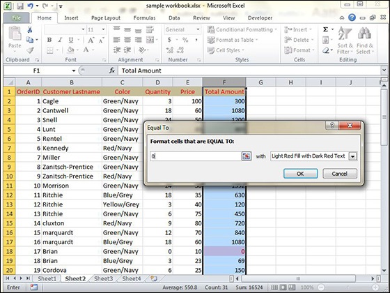
Highlight Cells Rules − It opens a continuation menu with various options for defining the formatting rules that highlight the cells in the cell selection that contain certain values, text, or dates, or that have values greater or less than a particular value, or that fall within a certain ranges of values.
Suppose you want to find cell with Amount 0 and Mark them as red.Choose Range of cell » Home Tab » Conditional Formatting DropDown » Highlight Cell Rules » Equal To.
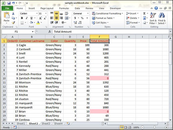
After Clicking ok, the cells with value zero are marked as red.
-
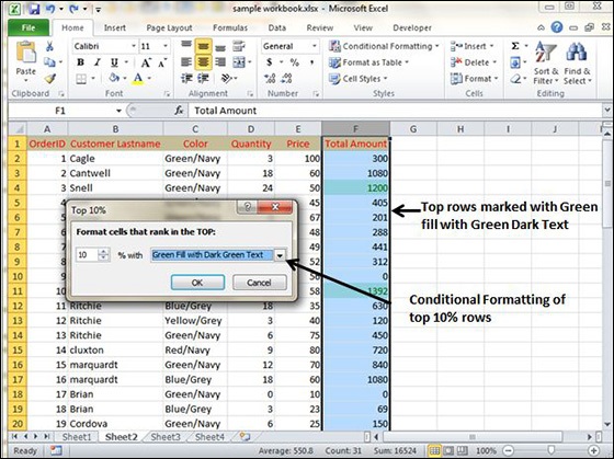
Top/Bottom Rules − It opens a continuation menu with various options for defining the formatting rules that highlight the top and bottom values, percentages, and above and below average values in the cell selection.
Suppose you want to highlight the top 10% rows you can do this with these Top/Bottom rules.
-
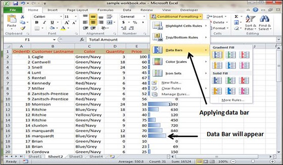
Data Bars − It opens a palette with different color data bars that you can apply to the cell selection to indicate their values relative to each other by clicking the data bar thumbnail.
With this conditional Formatting data Bars will appear in each cell.
-
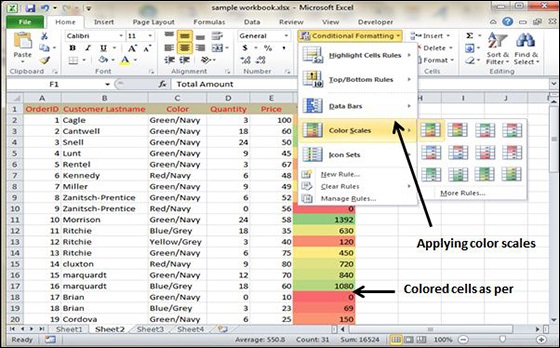
Color Scales − It opens a palette with different three- and two-colored scales that you can apply to the cell selection to indicate their values relative to each other by clicking the color scale thumbnail.
See the below screenshot with Color Scales, conditional formatting applied.
-
Icon Sets − It opens a palette with different sets of icons that you can apply to the cell selection to indicate their values relative to each other by clicking the icon set.
See the below screenshot with Icon Sets conditional formatting applied.
![]()
-
New Rule − It opens the New Formatting Rule dialog box, where you define a custom conditional formatting rule to apply to the cell selection.
-
Clear Rules − It opens a continuation menu, where you can remove the conditional formatting rules for the cell selection by clicking the Selected Cells option, for the entire worksheet by clicking the Entire Sheet option, or for just the current data table by clicking the This Table option.
-
Manage Rules − It opens the Conditional Formatting Rules Manager dialog box, where you edit and delete particular rules as well as adjust their rule precedence by moving them up or down in the Rules list box.
Creating Formulas in Excel 2010
Formulas in MS Excel
Formulas are the Bread and butter of worksheet. Without formula, worksheet will be just simple tabular representation of data. A formula consists of special code, which is entered into a cell. It performs some calculations and returns a result, which is displayed in the cell.
Formulas use a variety of operators and worksheet functions to work with values and text. The values and text used in formulas can be located in other cells, which makes changing data easy and gives worksheets their dynamic nature. For example, you can quickly change the data in a worksheet and formulas works.
Elements of Formulas
A formula can consist of any of these elements −
-
Mathematical operators, such as +(for addition) and *(for multiplication)
Example −
-
=A1+A2 Adds the values in cells A1 and A2.
-
-
Values or text
Example −
-
=200*0.5 Multiplies 200 times 0.15. This formula uses only values, and it always returns the same result as 100.
-
-
Cell references (including named cells and ranges)
Example −
-
=A1=C12 Compares cell A1 with cell C12. If the cells are identical, the formula returns TRUE; otherwise, it returns FALSE.
-
-
Worksheet functions (such as SUMor AVERAGE)
Example −
-
=SUM(A1:A12) Adds the values in the range A1:A12.
-
Creating Formula
For creating a formula you need to type in the Formula Bar. Formula begins with ‘=’ sign. When building formulas manually, you can either type in the cell addresses or you can point to them in the worksheet. Using the Pointing method to supply the cell addresses for formulas is often easier and more powerful method of formula building. When you are using built-in functions, you click the cell or drag through the cell range that you want to use when defining the function’s arguments in the Function Arguments dialog box. See the below screen shot.
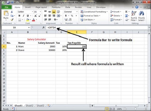
As soon as you complete a formula entry, Excel calculates the result, which is then displayed inside the cell within the worksheet (the contents of the formula, however, continue to be visible on the Formula bar anytime the cell is active). If you make an error in the formula that prevents Excel from being able to calculate the formula at all, Excel displays an Alert dialog box suggesting how to fix the problem.
Copying Formulas in Excel 2010
Copying Formulas in MS Excel
Copying formulas is one of the most common tasks that you do in a typical spreadsheet that relies primarily on formulas. When a formula uses cell references rather than constant values, Excel makes the task of copying an original formula to every place that requires a similar formula.
Relative Cell Addresses
MS Excel does it automatically adjusting the cell references in the original formula to suit the position of the copies that you make. It does this through a system known as relative cell addresses, where by the column references in the cell address in the formula change to suit their new column position and the row references change to suit their new row position.
Let us see this with the help of example. Suppose we want the sum of all the rows at last, then we will write a formula for first column i.e. B. We want sum of the rows from 3 to 8 in the 9th row.
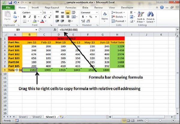
After writing formula in the 9th row, we can drag it to remaining columns and the formula gets copied. After dragging we can see the formula in the remaining columns as below.
-
column C : =SUM(C3:C8)
-
column D : =SUM(D3:D8)
-
column E : =SUM(E3:E8)
-
column F : =SUM(F3:F8)
-
column G : =SUM(G3:G8)
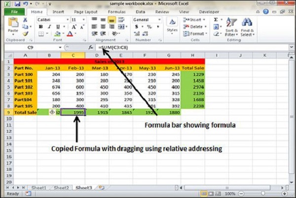
Formula Reference in Excel 2010
Cell References in Formulas
Most formulas you create include references to cells or ranges. These references enable your formulas to work dynamically with the data contained in those cells or ranges. For example, if your formula refers to cell C2 and you change the value contained in C2, the formula result reflects new value automatically. If you didn’t use references in your formulas, you would need to edit the formulas themselves in order to change the values used in the formulas.
When you use a cell (or range) reference in a formula, you can use three types of references − relative, absolute, and mixed references.
Relative Cell References
The row and column references can change when you copy the formula to another cell because the references are actually offsets from the current row and column. By default, Excel creates relative cell references in formulas.
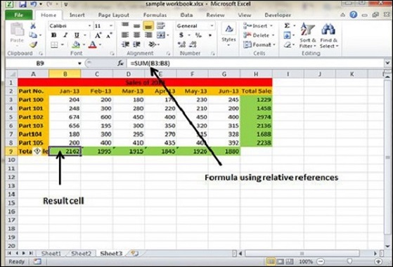
Absolute Cell References
The row and column references do not change when you copy the formula because the reference is to an actual cell address. An absolute reference uses two dollar signs in its address: one for the column letter and one for the row number (for example, $A$5).
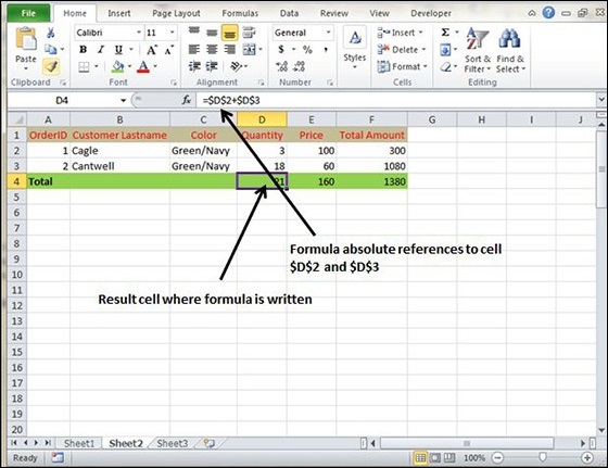
Mixed Cell References
Both the row or column reference is relative and the other is absolute. Only one of the address parts is absolute (for example, $A5 or A$5).
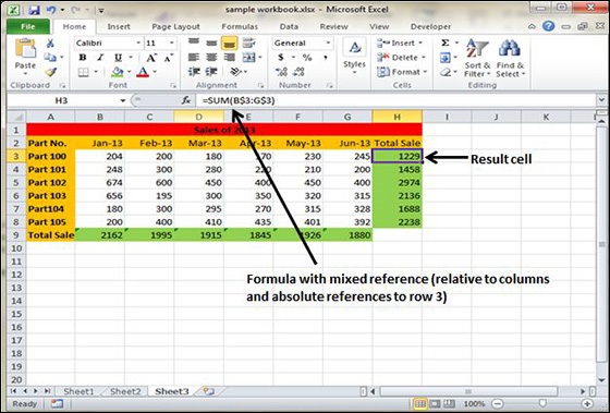
Using Functions in Excel 2010
Functions in Formula
Many formulas you create use available worksheet functions. These functions enable you to greatly enhance the power of your formulas and perform calculations that are difficult if you use only the operators. For example, you can use the LOG or SIN function to calculate the Logarithm or Sin ratio. You can’t do this complicated calculation by using the mathematical operators alone.
Using Functions
When you type = sign and then type any alphabet you will see the searched functions as below.
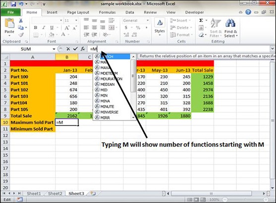
Suppose you need to determine the largest value in a range. A formula can’t tell you the answer without using a function. We will use formula that uses the MAX function to return the largest value in the range B3:B8 as =MAX(A1:D100).
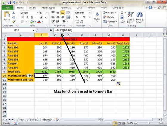
Another example of functions. Suppose you want to find if the cell of month is greater than 1900 then we can give Bonus to Sales representative. The we can achieve it with writing formula with IF functions as =IF(B9>1900,»Yes»,»No»)
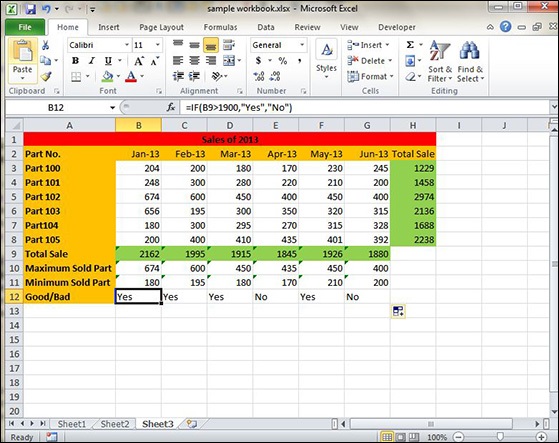
Function Arguments
In the above examples, you may have noticed that all the functions used parentheses. The information inside the parentheses is the list of arguments.
Functions vary in how they use arguments. Depending on what it has to do, a function may use.
-
No arguments − Examples − Now(), Date(), etc.
-
One argument − UPPER(), LOWER(), etc.
-
A fixed number of arguments − IF(), MAX(), MIN(), AVERGAGE(), etc.
-
Infinite number of arguments
-
Optional arguments
Built-in Functions in Excel 2010
Built In Functions
MS Excel has many built in functions, which we can use in our formula. To see all the functions by category, choose Formulas Tab » Insert Function. Then Insert function Dialog appears from which we can choose the function.
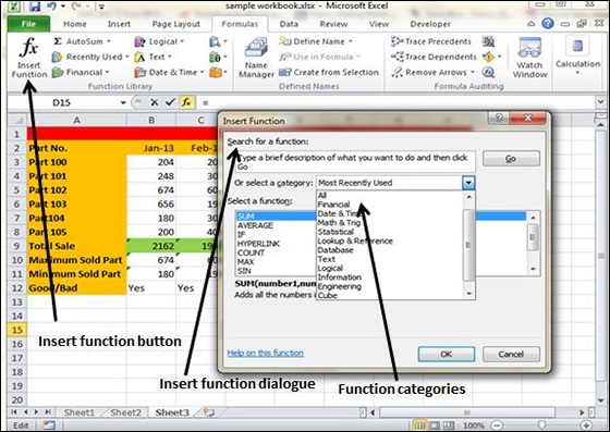
Functions by Categories
Let us see some of the built in functions in MS Excel.
-
Text Functions
-
LOWER − Converts all characters in a supplied text string to lower case
-
UPPER − Converts all characters in a supplied text string to upper case
-
TRIM − Removes duplicate spaces, and spaces at the start and end of a text string
-
CONCATENATE − Joins together two or more text strings.
-
LEFT − Returns a specified number of characters from the start of a supplied text string.
-
MID − Returns a specified number of characters from the middle of a supplied text string
-
RIGHT − Returns a specified number of characters from the end of a supplied text string.
-
LEN − Returns the length of a supplied text string
-
FIND − Returns the position of a supplied character or text string from within a supplied text string (case-sensitive).
-
-
Date & Time
-
DATE − Returns a date, from a user-supplied year, month and day.
-
TIME − Returns a time, from a user-supplied hour, minute and second.
-
DATEVALUE − Converts a text string showing a date, to an integer that represents the date in Excel’s date-time code.
-
TIMEVALUE − Converts a text string showing a time, to a decimal that represents the time in Excel.
-
NOW − Returns the current date & time.
-
TODAY − Returns today’s date.
-
-
Statistical
-
MAX − Returns the largest value from a list of supplied numbers.
-
MIN − Returns the smallest value from a list of supplied numbers.
-
AVERAGE − Returns the Average of a list of supplied numbers.
-
COUNT − Returns the number of numerical values in a supplied set of cells or values.
-
COUNTIF − Returns the number of cells (of a supplied range), that satisfies a given criteria.
-
SUM − Returns the sum of a supplied list of numbers
-
-
Logical
-
AND − Tests a number of user-defined conditions and returns TRUE if ALL of the conditions evaluate to TRUE, or FALSE otherwise
-
OR − Tests a number of user-defined conditions and returns TRUE if ANY of the conditions evaluate to TRUE, or FALSE otherwise.
-
NOT − Returns a logical value that is the opposite of a user supplied logical value or expression i.e. returns FALSE if the supplied argument is TRUE and returns TRUE if the supplied argument is FAL
-
-
Math & Trig
-
ABS − Returns the absolute value (i.e. the modulus) of a supplied number.
-
SIGN − Returns the sign (+1, -1 or 0) of a supplied number.
-
SQRT − Returns the positive square root of a given number.
-
MOD − Returns the remainder from a division between two supplied numbers.
-
Data Filtering in Excel 2010
Filters in MS Excel
Filtering data in MS Excel refers to displaying only the rows that meet certain conditions. (The other rows gets hidden.)
Using the store data, if you are interested in seeing data where Shoe Size is 36, then you can set filter to do this. Follow the below mentioned steps to do this.
-
Place a cursor on the Header Row.
-
Choose Data Tab » Filter to set filter.
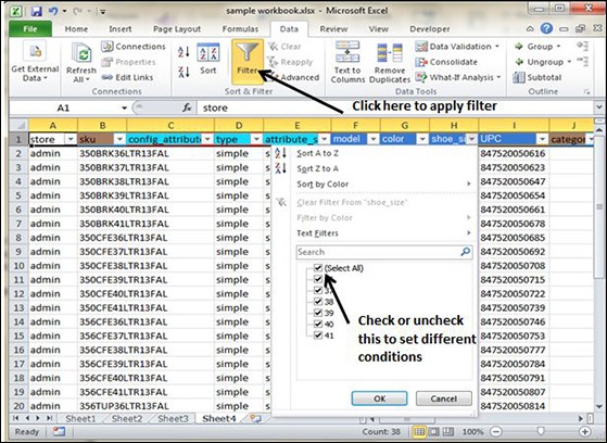
-
Click the drop-down arrow in the Area Row Header and remove the check mark from Select All, which unselects everything.
-
Then select the check mark for Size 36 which will filter the data and displays data of Shoe Size 36.
-
Some of the row numbers are missing; these rows contain the filtered (hidden) data.
-
There is drop-down arrow in the Area column now shows a different graphic — an icon that indicates the column is filtered.
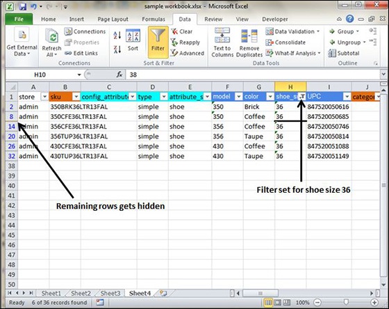
Using Multiple Filters
You can filter the records by multiple conditions i.e. by multiple column values. Suppose after size 36 is filtered, you need to have the filter where color is equal to Coffee. After setting filter for Shoe Size, choose Color column and then set filter for color.
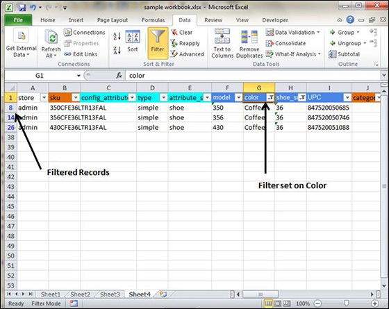
Data Sorting in Excel 2010
Sorting in MS Excel
Sorting data in MS Excel rearranges the rows based on the contents of a particular column. You may want to sort a table to put names in alphabetical order. Or, maybe you want to sort data by Amount from smallest to largest or largest to smallest.
To Sort the data follow the steps mentioned below.
- Select the Column by which you want to sort data.
- Choose Data Tab » Sort Below dialog appears.
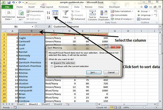
-
If you want to sort data based on a selected column, Choose Continue with the selection or if you want sorting based on other columns, choose Expand Selection.
-
You can Sort based on the below Conditions.
-
Values − Alphabetically or numerically.
-
Cell Color − Based on Color of Cell.
-
Font Color − Based on Font color.
-
Cell Icon − Based on Cell Icon.
-
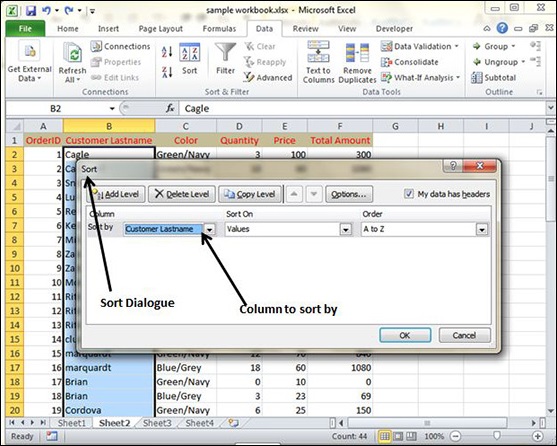
- Clicking Ok will sort the data.
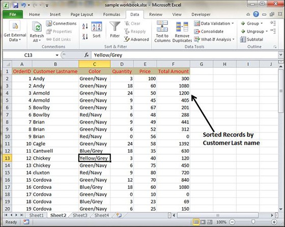
Sorting option is also available from the Home Tab. Choose Home Tab » Sort & Filter. You can see the same dialog to sort records.
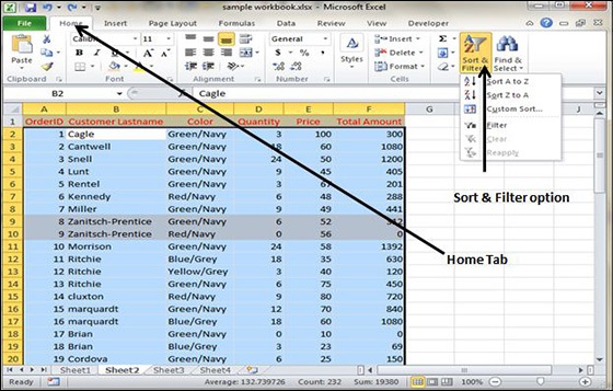
Using Ranges in Excel 2010
Ranges in MS Excel
A cell is a single element in a worksheet that can hold a value, some text, or a formula. A cell is identified by its address, which consists of its column letter and row number. For example, cell B1 is the cell in the second column and the first row.
A group of cells is called a range. You designate a range address by specifying its upper-left cell address and its lower-right cell address, separated by a colon.
Example of Ranges −
-
C24 − A range that consists of a single cell.
-
A1:B1 − Two cells that occupy one row and two columns.
-
A1:A100 − 100 cells in column A.
-
A1:D4 − 16 cells (four rows by four columns).
Selecting Ranges
You can select a range in several ways −
-
Press the left mouse button and drag, highlighting the range. Then release the mouse button. If you drag to the end of the screen, the worksheet will scroll.
-
Press the Shift key while you use the navigation keys to select a range.
-
Press F8 and then move the cell pointer with the navigation keys to highlight the range. Press F8 again to return the navigation keys to normal movement.
-
Type the cell or range address into the Name box and press Enter. Excel selects the cell or range that you specified.
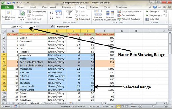
Selecting Complete Rows and Columns
When you need to select an entire row or column. You can select entire rows and columns in much the same manner as you select ranges −
-
Click the row or column border to select a single row or column.
-
To select multiple adjacent rows or columns, click a row or column border and drag to highlight additional rows or columns.
-
To select multiple (nonadjacent) rows or columns, press Ctrl while you click the row or column borders that you want.
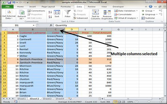
Data Validation in Excel 2010
Data Validation
MS Excel data validation feature allows you to set up certain rules that dictate what can be entered into a cell. For example, you may want to limit data entry in a particular cell to whole numbers between 0 and 10. If the user makes an invalid entry, you can display a custom message as shown below.
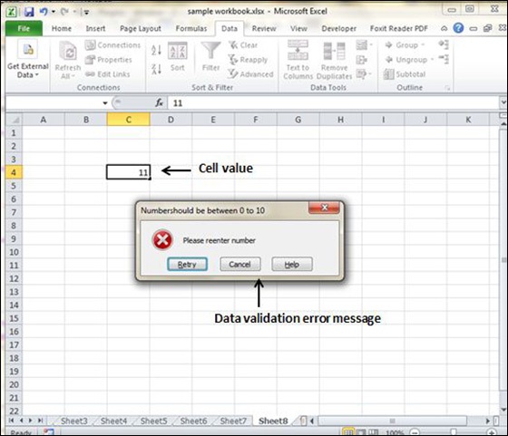
Validation Criteria
To specify the type of data allowable in a cell or range, follow the steps below, which shows all the three tabs of the Data Validation dialog box.
-
Select the cell or range.
-
Choose Data » Data Tools » Data Validation. Excel displays its Data Validation dialog box having 3 tabs settings, Input Message and Error alert.
Settings Tab
Here you can set the type of validation you need. Choose an option from the Allow drop-down list. The contents of the Data Validation dialog box will change, displaying controls based on your choice.
-
Any Value − Selecting this option removes any existing data validation.
-
Whole Number − The user must enter a whole number.For example, you can specify that the entry must be a whole number greater than or equal to 50.
-
Decimal − The user must enter a number. For example, you can specify that the entry must be greater than or equal to 10 and less than or equal to 20.
-
List − The user must choose from a list of entries you provide. You will create drop-down list with this validation. You have to give input ranges then those values will appear in the drop-down.
-
Date − The user must enter a date. You specify a valid date range from choices in the Data drop-down list. For example, you can specify that the entered data must be greater than or equal to January 1, 2013, and less than or equal to December 31, 2013.
-
Time − The user must enter a time. You specify a valid time range from choices in the Data drop-down list. For example, you can specify that the entered data must be later than 12:00 p.m.
-
Text Length − The length of the data (number of characters) is limited. You specify a valid length by using the Data drop-down list. For example, you can specify that the length of the entered data be 1 (a single alphanumeric character).
-
Custom − To use this option, you must supply a logical formula that determines the validity of the user’s entry (a logical formula returns either TRUE or FALSE).
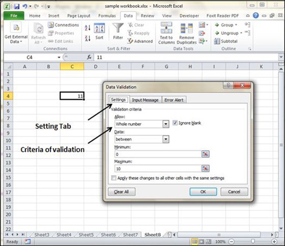
Input Message Tab
You can set the input help message with this tab. Fill the title and Input message of the Input message tab and the input message will appear when the cell is selected.
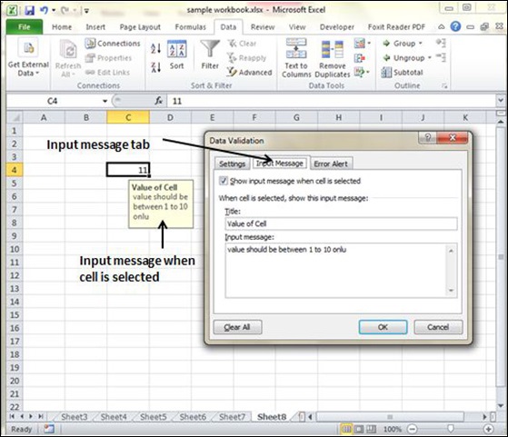
Error Alert Tab
You can specify an error message with this tab. Fill the title and error message. Select the style of the error as stop, warning or Information as per you need.
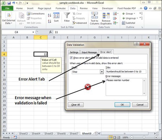
Using Styles in Excel 2010
Using Styles in MS Excel
With MS Excel 2010 Named styles make it very easy to apply a set of predefined formatting options to a cell or range. It saves time as well as make sure that look of the cells are consistent.
A Style can consist of settings for up to six different attributes −
- Number format
- Font (type, size, and color)
- Alignment (vertical and horizontal)
- Borders
- Pattern
- Protection (locked and hidden)
Now, let us see how styles are helpful. Suppose that you apply a particular style to some twenty cells scattered throughout your worksheet. Later, you realize that these cells should have a font size of 12 pt. rather than 14 pt. Rather than changing each cell, simply edit the style. All cells with that particular style change automatically.
Applying Styles
Choose Home » Styles » Cell Styles. Note that this display is a live preview, that is, as you move your mouse over the style choices, the selected cell or range temporarily displays the style. When you see a style you like, click it to apply the style to the selection.
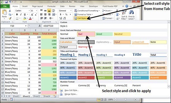
Creating Custom Style in MS Excel
We can create new custom style in Excel 2010. To create a new style, follow these steps −
- Select a cell and click on Cell styles from Home Tab.
- Click on New Cell Style and give style name.
- Click on Format to apply formatting to the cell.
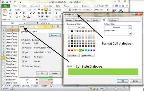
-
After applying formatting click on OK. This will add new style in the styles. You can view it on Home » Styles.
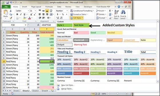
Using Themes in Excel 2010
Using Themes in MS Excel
To help users create more professional-looking documents, MS Excel has incorporated a concept known as document themes. By using themes, it is easy to specify the colors, fonts, and a variety of graphic effects in a document. And best of all, changing the entire look of your document is a breeze. A few mouse clicks is all it takes to apply a different theme and change the look of your workbook.
Applying Themes
Choose Page layout Tab » Themes Dropdown. Note that this display is a live preview, that is, as you move your mouse over the Theme, it temporarily displays the theme effect. When you see a style you like, click it to apply the style to the selection.
Creating Custom Theme in MS Excel
We can create new custom Theme in Excel 2010. To create a new style, follow these steps −
-
Click on the save current theme option under Theme in Page Layout Tab.
-
This will save the current theme to office folder.
-
You can browse the theme later to load the theme.
Using Templates in Excel 2010
Using Templates in MS Excel
Template is essentially a model that serves as the basis for something. An Excel template is a workbook that’s used to create other workbooks.
Viewing Available Templates
To view the Excel templates, choose File » New to display the available templates screen in Backstage View. You can select a template stored on your hard drive, or a template from Microsoft Office Online. If you choose a template from Microsoft Office Online, you must be connected to the Internet to download it. The Office Online Templates section contains a number of icons, which represents various categories of templates. Click an icon, and you’ll see the available templates. When you select a template thumbnail, you can see a preview in the right panel.
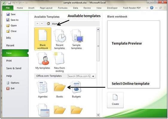
On-line Templates
These template data is available online at the Microsoft server. When you select the template and click on it, it will download the template data from Microsoft server and opens it as shown below.
Using Templates in MS Excel
Template is essentially a model that serves as the basis for something. An Excel template is a workbook that’s used to create other workbooks.
Viewing Available Templates
To view the Excel templates, choose File » New to display the available templates screen in Backstage View. You can select a template stored on your hard drive, or a template from Microsoft Office Online. If you choose a template from Microsoft Office Online, you must be connected to the Internet to download it. The Office Online Templates section contains a number of icons, which represents various categories of templates. Click an icon, and you’ll see the available templates. When you select a template thumbnail, you can see a preview in the right panel.
On-line Templates
These template data is available online at the Microsoft server. When you select the template and click on it, it will download the template data from Microsoft server and opens it as shown below.
Using Macros in Excel 2010
Macros in MS Excel
Macros enable you to automate almost any task that you can undertake in Excel 2010. By using macro recorder from View Tab » Macro Dropdown to record tasks that you perform routinely, you not only speed up the procedure considerably but you are assured that each step in a task is carried out the same way each and every time you perform a task.
To view macros choose View Tab » Macro dropdown.
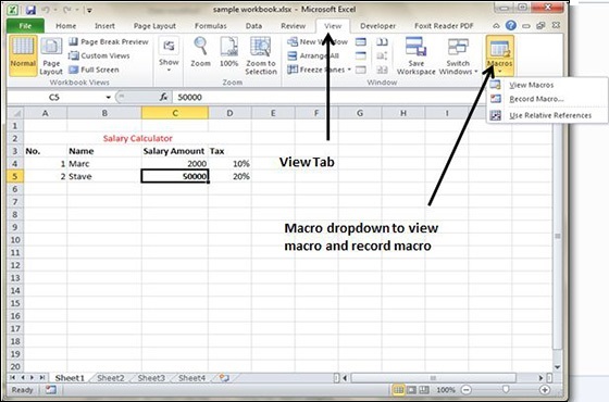
Macro Options
View tab contains a Macros command button to which a dropdown menu containing the following three options.
-
View Macros − Opens the Macro dialog box where you can select a macro to run or edit.
-
Record Macro − Opens the Record Macro dialog box where you define the settings for your new macro and then start the macro recorder; this is the same as clicking the Record Macro button on the Status bar.
-
Use Relative References − Uses relative cell addresses when recording a macro, making the macro more versatile by enabling you to run it in areas of a worksheet other than the ones originally used in the macro’s recording.
Creating Macros
You can create macros in one of two ways −
-
Use MS Excel’s macro recorder to record your actions as you undertake them in a worksheet.
-
Enter the instructions that you want to be followed in a VBA code in the Visual Basic Editor.
Now let’s create a simple macro that will automate the task of making cell content Bold and apply cell color.
- Choose View Tab » Macro dropdown.
- Click on Record Macro as below.
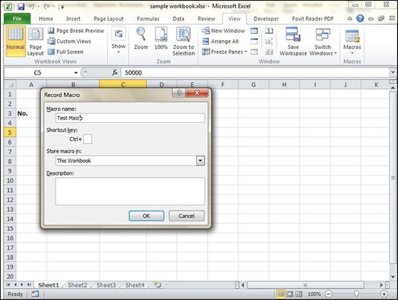
-
Now Macro recording will start.
-
Do the steps of action, which you want to perform repeatedly. Macro will record those steps.
-
You can stop the macro recording once done with all steps.
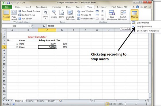
Edit Macro
You can edit the created Macro at any time. Editing macro will take you to the VBA programming editor.
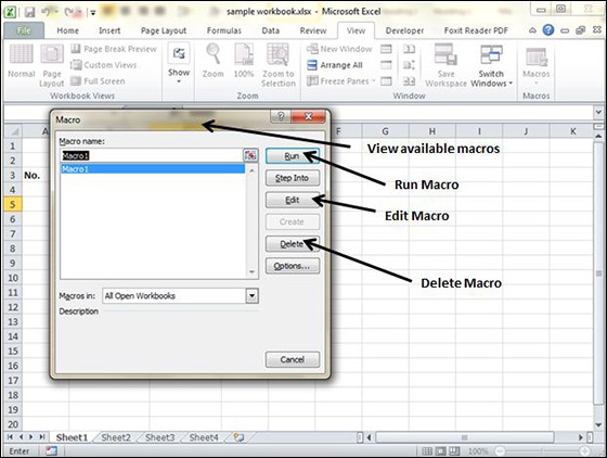
Adding Graphics in Excel 2010
Graphic Objects in MS Excel
MS Excel supports various types of graphic objects like Shapes gallery, SmartArt, Text Box, and WordArt available on the Insert tab of the Ribbon.Graphics are available in the Insert Tab. See the screenshots below for various available graphics in MS Excel 2010.
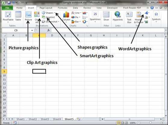
Insert Shape
-
Choose Insert Tab » Shapes dropdown.
-
Select the shape you want to insert. Click on shape to insert it.
-
To edit the inserted shape just drag the shape with the mouse. Shape will adjust the shape.
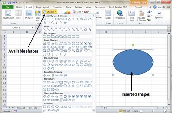
Insert Smart Art
-
Choose Insert Tab » SmartArt.
-
Clicking SmartArt will open the SmartArt dialogue as shown below in the screen-shot. Choose from the list of available smartArts.
-
Click on SmartArt to Insert it in the worksheet.
-
Edit the SmartArt as per your need.
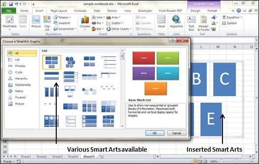
Insert Clip Art
-
Choose Insert Tab » Clip Art.
-
Clicking Clip Art will open the search box as shown in the below screen-shot. Choose from the list of available Clip Arts.
-
Click on Clip Art to Insert it in the worksheet.
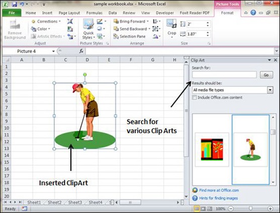
Insert Word Art
-
Choose Insert Tab » WordArt.
-
Select the style of WordArt, which you like and click it to enter a text in it.
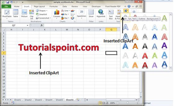
Cross Referencing in Excel 2010
Graphic Objects in MS Excel
When you have information spread across several different spreadsheets, it can seem a daunting task to bring all these different sets of data together into one meaningful list or table. This is where the Vlookup function comes into its own.
VLOOKUP
VlookUp searches for a value vertically down for the lookup table. VLOOKUP(lookup_value,table_array,col_index_num,range_lookup) has 4 parameters as below.
-
lookup_value − It is the user input. This is the value that the function uses to search on.
-
The table_array − It is the area of cells in which the table is located. This includes not only the column being searched on, but the data columns for which you are going to get the values that you need.
-
Col_index_num − It is the column of data that contains the answer that you want.
-
Range_lookup − It is a TRUE or FALSE value. When set to TRUE, the lookup function gives the closest match to the lookup_value without going over the lookup_value. When set to FALSE, an exact match must be found to the lookup_value or the function will return #N/A. Note, this requires that the column containing the lookup_value be formatted in ascending order.
VLOOKUP Example
Let’s look at a very simple example of cross-referencing two spreadsheets. Each spreadsheet contains information about the same group of people. The first spreadsheet has their dates of birth, and the second shows their favorite color. How do we build a list showing the person’s name, their date of birth and their favorite color? VLOOOKUP will help in this case. First of all, let us see data in both the sheets.
This is data in the first sheet
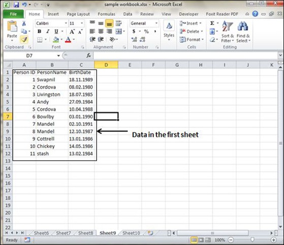
This is data in the second sheet
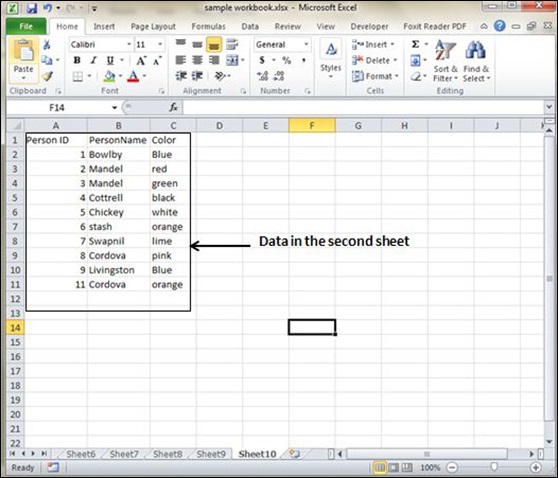
Now for finding the respective favorite color for that person from another sheet we need to vlookup the data. First argument to the VLOOKUP is lookup value (In this case it is person name). Second argument is the table array, which is table in the second sheet from B2 to C11. Third argument to VLOOKUP is Column index num, which is the answer we are looking for. In this case, it is 2 the color column number is 2. The fourth argument is True returning partial match or false returning exact match. After applying VLOOKUP formula it will calculate the color and the results are displayed as below.
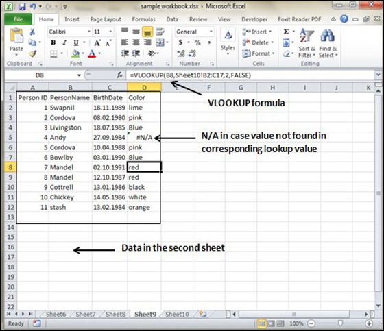
As you can see in the above screen-shot that results of VLOOKUP has searched for color in the second sheet table. It has returned #N/A in case where match is not found. In this case, Andy’s data is not present in the second sheet so it returned #N/A.
Printing Worksheets in Excel 2010
Quick Print
If you want to print a copy of a worksheet with no layout adjustment, use the Quick Print option. There are two ways in which we can use this option.
-
Choose File » Print (which displays the Print pane), and then click the Print button.
-
Press Ctrl+P and then click the Print button (or press Enter).
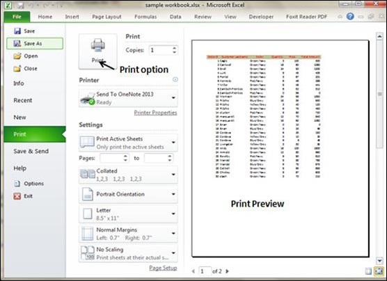
Adjusting Common Page Setup Settings
You can adjust the print settings available in the Page setup dialogue in different ways as discussed below. Page setup options include Page orientation, Page Size, Page Margins, etc.
-
The Print screen in Backstage View, displayed when you choose File » Print.
-
The Page Layout tab of the Ribbon.
Choosing Your Printer
To switch to a different printer, choose File » Print and use the drop-down control in the Printer section to select any other installed printer.
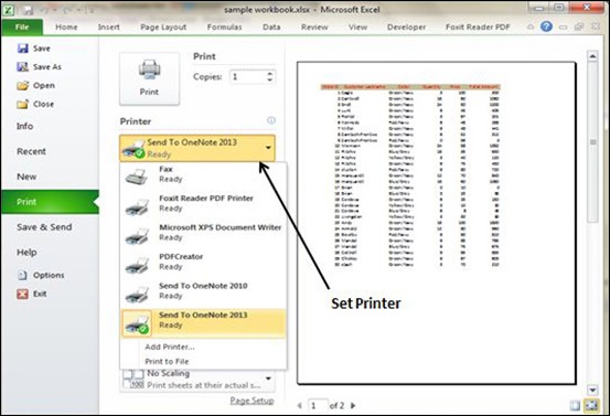
Specifying What You Want to Print
Sometimes you may want to print only a part of the worksheet rather than the entire active area. Choose File » Print and use the controls in the Settings section to specify what to print.
-
Active Sheets − Prints the active sheet or sheets that you selected.
-
Entire Workbook − Prints the entire workbook, including chart sheets.
-
Selection − Prints only the range that you selected before choosing File » Print.
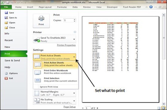
Email Workbooks MS Excel 2010
Email Workbook
MS Excel allows you to email the workbook very easily. To email the workbook to anyone, follow the below mentioned steps.
-
Choose File » Save and Send. It basically saves the document first and then the emails.
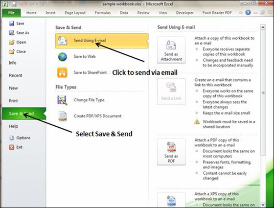
-
Click on Send using E-mail if your email system is configured. MS Outlook will open with the file as attachment in the New Email Window. You can send mail this workbook to anyone with valid email address.
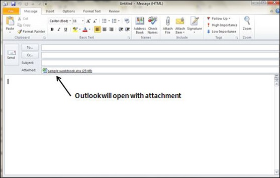
Translate Worksheet in Excel 2010
Translate Worksheet
You can translate the text written in a different language, such as phrases or paragraphs, individual words (by using the Mini Translator), or translate your whole file with MS Excel 2010.
Translation is available in the review tab of the ribbon in MS Excel 2010. You can quickly translate cell into different language with this option.
Performing Translation Step By Step
-
Select the content, which you want to translate to a different language.
-
Choose review tab » translation.
-
It will open the pane from which you can select the language to which you need to translate.
-
You need to have an internet connection for performing translation. It will translate using the Microsoft Translator.
-
Click on Insert to apply translation changes.
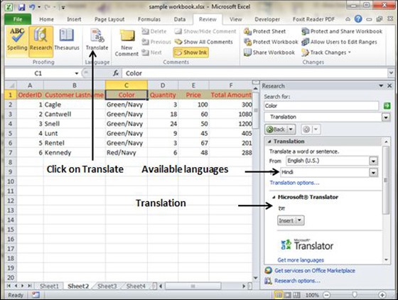
Workbook Security in Excel 2010
Workbook Security
We can apply security to the workbook by the concept of protection available in the Review Tab of ribbon. MS Excel’s protection-related features fall into three categories.
-
Worksheet protection − Protecting a worksheet from being modified, or restricting the modifications to certain users.
-
Workbook protection − Protecting a workbook from having sheets inserted or deleted, and also requiring the use of password to open the workbook.
Protect Worksheet
You may want to protect a worksheet for a variety of reasons. One reason is to prevent yourself or others from accidentally deleting the formulas or other critical data. A common scenario is to protect a worksheet, so that the data can be changed, but the formulas can’t be changed.
To protect a worksheet, choose Review » Changes group » Protect Sheet. Excel displays the Protect Sheet dialog box. Note that providing a password is optional. If you enter a password, that password will be required to unprotect the worksheet. You can select various options in which the sheet should be protected. Suppose we checked Format Cells option then Excel will not allow to format cells.
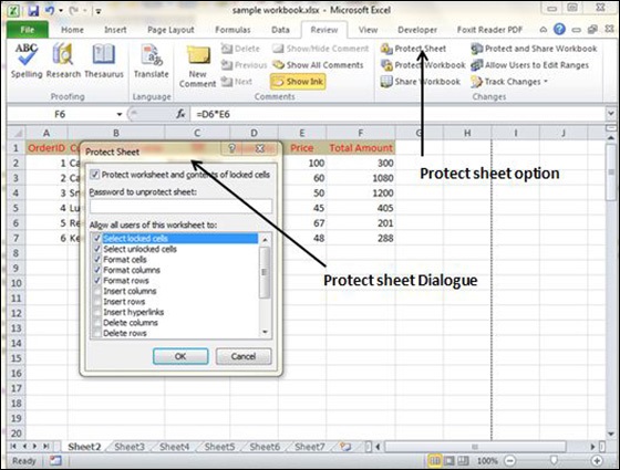
When somebody tries to format the cells, he or she will get the error as shown in the screenshot below.
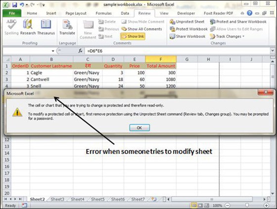
To unprotect a protected sheet, choose Review » Changes group » Unprotect Sheet. If the sheet was protected with a password, you’re prompted to enter that password.
Protecting a Workbook
Excel provides three ways to protect a workbook.
-
Requires a password to open the workbook.
-
Prevents the users from adding sheets, deleting sheets, hiding sheets, and unhiding sheets.
-
Prevents users from changing the size or position of windows.
Requiring a Password to Open a Workbook
Excel lets you save a workbook with a password. After doing so, whoever tries to open the workbook, must enter the password. To add a password to a workbook, follow these steps.
-
Choose File » Info » Protect Workbook » Encrypt With Password. Excel displays the Encrypt Document dialog box.
-
Type a password and click OK.
-
Type the password again and click OK.
-
Save the workbook.
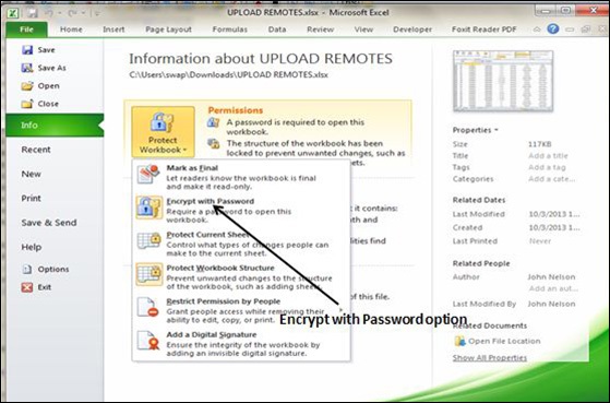
To remove a password from a workbook, repeat the same procedure. In Step 2, however, delete the existing password symbols.
Protecting Workbook’s Structure and Windows
To prevent others (or yourself) from performing certain actions in a workbook, you can protect the workbook’s structure and windows. When a workbook’s structure and windows are protected, the user may not Add a sheet, Delete a sheet, Hide a sheet, unhide a sheet, etc., and may not be allowed to change the size or position of a workbook’s windows respectively.
To protect a worksheet’s structure and windows, follow the below mentioned steps.
-
Choose Review » Changes group » Protect Workbook to display the Protect Workbook dialog box.
-
In the Protect Workbook dialog box, select the Structure check box and Windows check box.
-
(Optional) Enter a password.
-
Click OK.
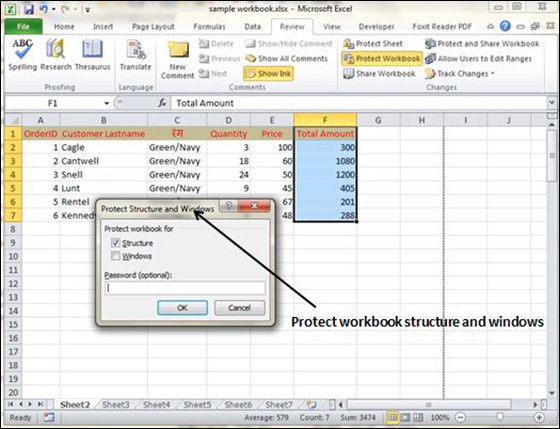
Data Tables in Excel 2010
Data Tables
In Excel, a Data Table is a way to see different results by altering an input cell in your formula. Data tables are available in Data Tab » What-If analysis dropdown » Data table in MS Excel.
Data Table with Example
Now, let us see data table concept with an example. Suppose you have the Price and quantity of many values. Also, you have the discount for that as third variable for calculating the Net Price. You can keep the Net Price value in the organized table format with the help of the data table. Your Price runs horizontally to the right while quantity runs vertically down. We are using a formula to calculate the Net Price as Price multiplied by Quantity minus total discount (Quantity * Discount for each quantity).
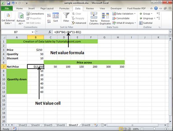
Now, for creation of data table select the range of data table. Choose Data Tab » What-If analysis dropdown » Data table. It will give you dialogue asking for Input row and Input Column. Give the Input row as Price cell (In this case cell B3) and Input column as quantity cell (In this case cell B4). Please see the below screen-shot.
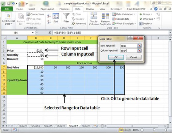
Clicking OK will generate data table as shown in the below screen-shot. It will generate the table formula. You can change the price horizontally or quantity vertically to see the change in the Net Price.
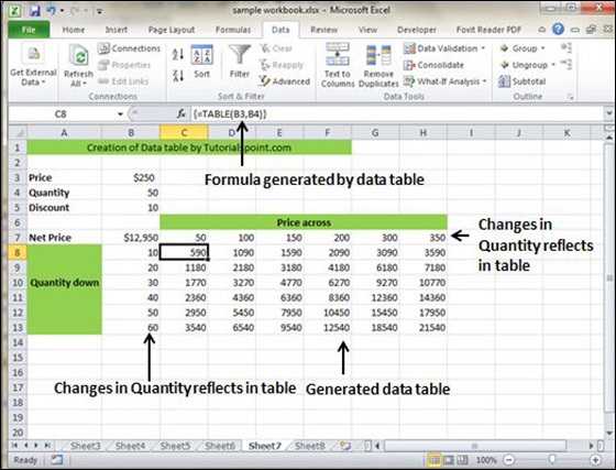
Pivot Tables in Excel 2010
Pivot Tables
A pivot table is essentially a dynamic summary report generated from a database. The database can reside in a worksheet (in the form of a table) or in an external data file. A pivot table can help transform endless rows and columns of numbers into a meaningful presentation of the data. Pivot tables are very powerful tool for summarized analysis of the data.
Pivot tables are available under Insert tab » PivotTable dropdown » PivotTable.
Pivot Table Example
Now, let us see Pivot table with the help of example. Suppose you have huge data of voters and you want to see the summarized data of voter Information per party, then you can use the Pivot table for it. Choose Insert tab » Pivot Table to insert pivot table. MS Excel selects the data of the table. You can select the pivot table location as existing sheet or new sheet.
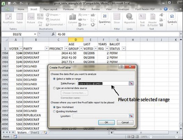
This will generate the Pivot table pane as shown below. You have various options available in the Pivot table pane. You can select fields for the generated pivot table.
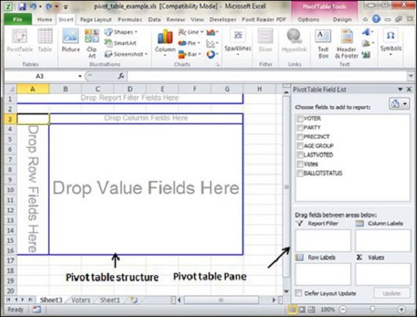
-
Column labels − A field that has a column orientation in the pivot table. Each item in the field occupies a column.
-
Report Filter − You can set the filter for the report as year, then data gets filtered as per the year.
-
Row labels − A field that has a row orientation in the pivot table. Each item in the field occupies a row.
-
Values area − The cells in a pivot table that contain the summary data. Excel offers several ways to summarize the data (sum, average, count, and so on).
After giving input fields to the pivot table, it generates the pivot table with the data as shown below.
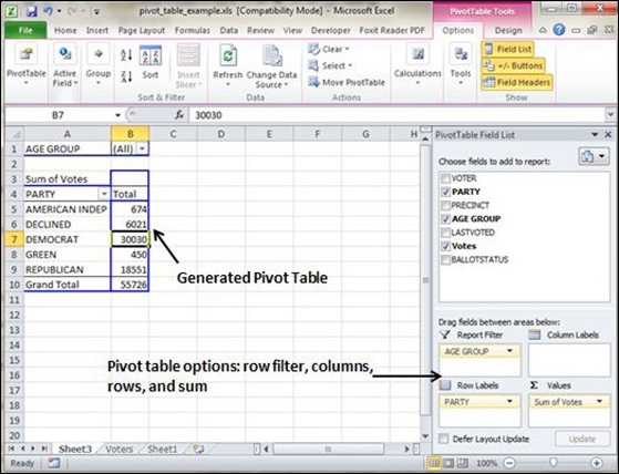
Simple Charts in Excel 2010
Charts
A chart is a visual representation of numeric values. Charts (also known as graphs) have been an integral part of spreadsheets. Charts generated by early spreadsheet products were quite crude, but thy have improved significantly over the years. Excel provides you with the tools to create a wide variety of highly customizable charts. Displaying data in a well-conceived chart can make your numbers more understandable. Because a chart presents a picture, charts are particularly useful for summarizing a series of numbers and their interrelationships.
Types of Charts
There are various chart types available in MS Excel as shown in the below screen-shot.
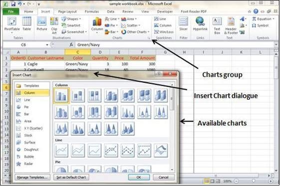
-
Column − Column chart shows data changes over a period of time or illustrates comparisons among items.
-
Bar − A bar chart illustrates comparisons among individual items.
-
Pie − A pie chart shows the size of items that make up a data series, proportional to the sum of the items. It always shows only one data series and is useful when you want to emphasize a significant element in the data.
-
Line − A line chart shows trends in data at equal intervals.
-
Area − An area chart emphasizes the magnitude of change over time.
-
X Y Scatter − An xy (scatter) chart shows the relationships among the numeric values in several data series, or plots two groups of numbers as one series of xy coordinates.
-
Stock − This chart type is most often used for stock price data, but can also be used for scientific data (for example, to indicate temperature changes).
-
Surface − A surface chart is useful when you want to find the optimum combinations between two sets of data. As in a topographic map, colors and patterns indicate areas that are in the same range of values.
-
Doughnut − Like a pie chart, a doughnut chart shows the relationship of parts to a whole; however, it can contain more than one data series.
-
Bubble − Data that is arranged in columns on a worksheet, so that x values are listed in the first column and corresponding y values and bubble size values are listed in adjacent columns, can be plotted in a bubble chart.
-
Radar − A radar chart compares the aggregate values of a number of data series.
Creating Chart
To create charts for the data by below mentioned steps.
-
Select the data for which you want to create the chart.
-
Choose Insert Tab » Select the chart or click on the Chart group to see various chart types.
-
Select the chart of your choice and click OK to generate the chart.
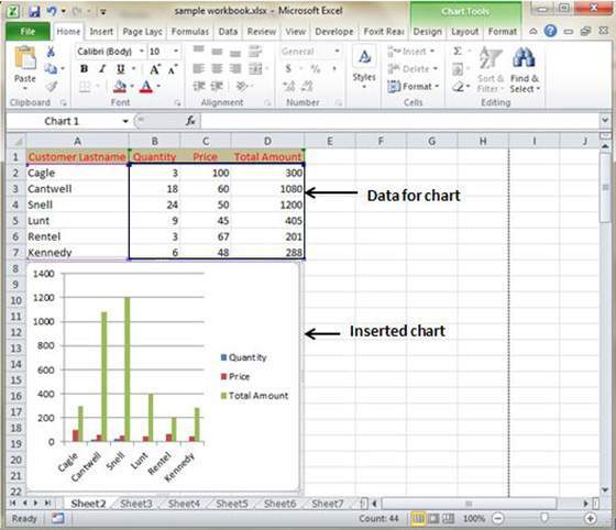
Editing Chart
You can edit the chart at any time after you have created it.
-
You can select the different data for chart input with Right click on chart » Select data. Selecting new data will generate the chart as per the new data, as shown in the below screen-shot.
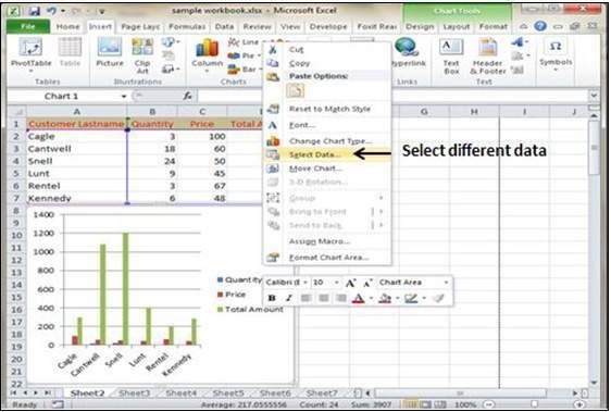
-
You can change the X axis of the chart by giving different inputs to X-axis of chart.
-
You can change the Y axis of chart by giving different inputs to Y-axis of chart.
Pivot Charts Excel 2010
Pivot Charts
A pivot chart is a graphical representation of a data summary, displayed in a pivot table. A pivot chart is always based on a pivot table. Although Excel lets you create a pivot table and a pivot chart at the same time, you can’t create a pivot chart without a pivot table. All Excel charting features are available in a pivot chart.
Pivot charts are available under Insert tab » PivotTable dropdown » PivotChart.
Pivot Chart Example
Now, let us see Pivot table with the help of an example. Suppose you have huge data of voters and you want to see the summarized view of the data of voter Information per party in the form of charts, then you can use the Pivot chart for it. Choose Insert tab » Pivot Chart to insert the pivot table.
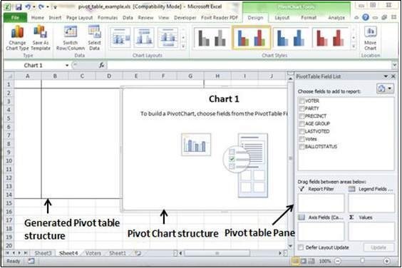
MS Excel selects the data of the table. You can select the pivot chart location as an existing sheet or a new sheet. Pivot chart depends on automatically created pivot table by the MS Excel. You can generate the pivot chart in the below screen-shot.
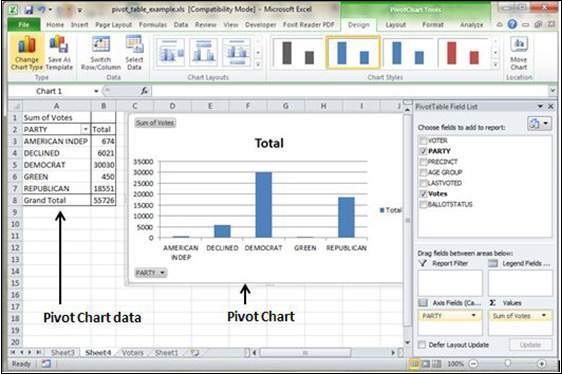
Keyboard Shortcuts in Excel 2010
MS Excel Keyboard Short-cuts
MS Excel offers many keyboard short-cuts. If you are familiar with windows operating system, you should be aware of most of them. Below is the list of all the major shortcut keys in Microsoft Excel.
-
Ctrl + A − Selects all contents of the worksheet.
-
Ctrl + B − Bold highlighted selection.
-
Ctrl + I − Italicizes the highlighted selection.
-
Ctrl + K − Inserts link.
-
Ctrl + U − Underlines the highlighted selection.
-
Ctrl + 1 − Changes the format of selected cells.
-
Ctrl + 5 − Strikethrough the highlighted selection.
-
Ctrl + P − Brings up the print dialog box to begin printing.
-
Ctrl + Z − Undo last action.
-
Ctrl + F3 − Opens Excel Name Manager.
-
Ctrl + F9 − Minimizes the current window.
-
Ctrl + F10 − Maximize currently selected window.
-
Ctrl + F6 − Switches between open workbooks or windows.
-
Ctrl + Page up − Moves between Excel work sheets in the same Excel document.
-
Ctrl + Page down − Moves between Excel work sheets in the same Excel document.
-
Ctrl + Tab − Moves between Two or more open Excel files.
-
Alt + = − Creates a formula to sum all of the above cells
-
Ctrl + ‘ − Inserts the value of the above cell into cell currently selected.
-
Ctrl + Shift + ! − Formats the number in comma format.
-
Ctrl + Shift + $ − Formats the number in currency format.
-
Ctrl + Shift + # − Formats the number in date format.
-
Ctrl + Shift + % − Formats the number in percentage format.
-
Ctrl + Shift + ^ − Formats the number in scientific format.
-
Ctrl + Shift + @ − Formats the number in time format.
-
Ctrl + Arrow key − Moves to the next section of text.
-
Ctrl + Space − Selects the entire column.
-
Shift + Space − Selects the entire row.
-
Ctrl + — − Deletes the selected column or row.
-
Ctrl + Shift + = − Inserts a new column or row.
-
Ctrl + Home − Moves to cell A1.
-
Ctrl + ~ − Switches between showing Excel formulas or their values in cells.
-
F2 − Edits the selected cell.
-
F3 − After a name has been created F3 will paste names.
-
F4 − Repeat last action. For example, if you changed the color of text in another cell pressing F4 will change the text in cell to the same color.
-
F5 − Goes to a specific cell. For example, C6.
-
F7 − Spell checks the selected text or document.
-
F11 − Creates chart from the selected data.
-
Ctrl + Shift + ; − Enters the current time.
-
Ctrl + ; − Enters the current date.
-
Alt + Shift + F1 − Inserts New Worksheet.
-
Alt + Enter − While typing text in a cell pressing Alt + Enter will move to the next line allowing for multiple lines of text in one cell.
-
Shift + F3 − Opens the Excel formula window.
-
Shift + F5 − Brings up the search box.
In this Microsoft Excel tutorial, we will learn the Microsoft Exel basics. These Microsoft Excel notes will help you learn every MS Excel concepts. Let’s start with the introduction:
What is Microsoft Excel?
Microsoft Excel is a spreadsheet program used to record and analyze numerical and statistical data. Microsoft Excel provides multiple features to perform various operations like calculations, pivot tables, graph tools, macro programming, etc. It is compatible with multiple OS like Windows, macOS, Android and iOS.
A Excel spreadsheet can be understood as a collection of columns and rows that form a table. Alphabetical letters are usually assigned to columns, and numbers are usually assigned to rows. The point where a column and a row meet is called a cell. The address of a cell is given by the letter representing the column and the number representing a row.
Why Should I Learn Microsoft Excel?
We all deal with numbers in one way or the other. We all have daily expenses which we pay for from the monthly income that we earn. For one to spend wisely, they will need to know their income vs. expenditure. Microsoft Excel comes in handy when we want to record, analyze and store such numeric data. Let’s illustrate this using the following image.

Where can I get Microsoft Excel?
There are number of ways in which you can get Microsoft Excel. You can buy it from a hardware computer shop that also sells software. Microsoft Excel is part of the Microsoft Office suite of programs. Alternatively, you can download it from the Microsoft website but you will have to buy the license key.
In this Microsoft Excel tutorial, we are going to cover the following topics about MS Excel.
- How to Open Microsoft Excel?
- Understanding the Ribbon
- Understanding the worksheet
- Customization Microsoft Excel Environment
- Important Excel shortcuts
How to Open Microsoft Excel?
Running Excel is not different from running any other Windows program. If you are running Windows with a GUI like (Windows XP, Vista, and 7) follow the following steps.
- Click on start menu
- Point to all programs
- Point to Microsoft Excel
- Click on Microsoft Excel
Alternatively, you can also open it from the start menu if it has been added there. You can also open it from the desktop shortcut if you have created one.
For this tutorial, we will be working with Windows 8.1 and Microsoft Excel 2013. Follow the following steps to run Excel on Windows 8.1
- Click on start menu
- Search for Excel N.B. even before you even typing, all programs starting with what you have typed will be listed.
- Click on Microsoft Excel
The following image shows you how to do this

Understanding the Ribbon
The ribbon provides shortcuts to commands in Excel. A command is an action that the user performs. An example of a command is creating a new document, printing a documenting, etc. The image below shows the ribbon used in Excel 2013.

Ribbon components explained
Ribbon start button – it is used to access commands i.e. creating new documents, saving existing work, printing, accessing the options for customizing Excel, etc.
Ribbon tabs – the tabs are used to group similar commands together. The home tab is used for basic commands such as formatting the data to make it more presentable, sorting and finding specific data within the spreadsheet.
Ribbon bar – the bars are used to group similar commands together. As an example, the Alignment ribbon bar is used to group all the commands that are used to align data together.
Understanding the worksheet (Rows and Columns, Sheets, Workbooks)
A worksheet is a collection of rows and columns. When a row and a column meet, they form a cell. Cells are used to record data. Each cell is uniquely identified using a cell address. Columns are usually labelled with letters while rows are usually numbers.
A workbook is a collection of worksheets. By default, a workbook has three cells in Excel. You can delete or add more sheets to suit your requirements. By default, the sheets are named Sheet1, Sheet2 and so on and so forth. You can rename the sheet names to more meaningful names i.e. Daily Expenses, Monthly Budget, etc.

Customization Microsoft Excel Environment
Personally I like the black colour, so my excel theme looks blackish. Your favourite colour could be blue, and you too can make your theme colour look blue-like. If you are not a programmer, you may not want to include ribbon tabs i.e. developer. All this is made possible via customizations. In this sub-section, we are going to look at;
- Customization the ribbon
- Setting the colour theme
- Settings for formulas
- Proofing settings
- Save settings
Customization of ribbon

The above image shows the default ribbon in Excel 2013. Let’s start with customization the ribbon, suppose you do not wish to see some of the tabs on the ribbon, or you would like to add some tabs that are missing such as the developer tab. You can use the options window to achieve this.
- Click on the ribbon start button
- Select options from the drop down menu. You should be able to see an Excel Options dialog window
- Select the customize ribbon option from the left-hand side panel as shown below

- On your right-hand side, remove the check marks from the tabs that you do not wish to see on the ribbon. For this example, we have removed Page Layout, Review, and View tab.
- Click on the “OK” button when you are done.
Your ribbon will look as follows

Adding custom tabs to the ribbon
You can also add your own tab, give it a custom name and assign commands to it. Let’s add a tab to the ribbon with the text Guru99

- Right click on the ribbon and select Customize the Ribbon. The dialogue window shown above will appear
- Click on new tab button as illustrated in the animated image below
- Select the newly created tab
- Click on Rename button
- Give it a name of Guru99
- Select the New Group (Custom) under Guru99 tab as shown in the image below
- Click on Rename button and give it a name of My Commands
- Let’s now add commands to my ribbon bar
- The commands are listed on the middle panel
- Select All chart types command and click on Add button
- Click on OK
Your ribbon will look as follows

Setting the colour theme
To set the color-theme for your Excel sheet you have to go to Excel ribbon, and click on à File àOption command. It will open a window where you have to follow the following steps.

- The general tab on the left-hand panel will be selected by default.
- Look for colour scheme under General options for working with Excel
- Click on the colour scheme drop-down list and select the desired colour
- Click on OK button
Settings for formulas
This option allows you to define how Excel behaves when you are working with formulas. You can use it to set options i.e. autocomplete when entering formulas, change the cell referencing style and use numbers for both columns and rows and other options.

If you want to activate an option, click on its check box. If you want to deactivate an option, remove the mark from the checkbox. You can this option from the Options dialogue window under formulas tab from the left-hand side panel
Proofing settings

This option manipulates the entered text entered into excel. It allows setting options such as the dictionary language that should be used when checking for wrong spellings, suggestions from the dictionary, etc. You can this option from the options dialogue window under the proofing tab from the left-hand side panel
Save settings

This option allows you to define the default file format when saving files, enable auto recovery in case your computer goes off before you could save your work, etc. You can use this option from the Options dialogue window under save tab from the left-hand side panel
Important Excel shortcuts
| Ctrl + P | used to open the print dialogue window |
| Ctrl + N | creates a new workbook |
| Ctrl + S | saves the current workbook |
| Ctrl + C | copy contents of current select |
| Ctrl + V | paste data from the clipboard |
| SHIFT + F3 | displays the function insert dialog window |
| SHIFT + F11 | Creates a new worksheet |
| F2 | Check formula and cell range covered |
Best Practices when working with Microsoft Excel
- Save workbooks with backward compatibility in mind. If you are not using the latest features in higher versions of Excel, you should save your files in 2003 *.xls format for backwards compatibility
- Use description names for columns and worksheets in a workbook
- Avoid working with complex formulas with many variables. Try to break them down into small managed results that you can use to build on
- Use built-in functions whenever you can instead of writing your own formulas
Summary
- Introduction of MS Excel : Microsoft Excel is a powerful spreadsheet program used to record, manipulate, store numeric data and it can be customized to match your preferences
- The ribbon is used to access various commands in Excel
- The options dialogue window allows you to customize a number of items i.e. the ribbon, formulas, proofing, save, etc.
Microsoft Excel know-how is so expected that it hardly warrants a line on a resume anymore. But how well do you really know how to use it?
Marketing is more data-driven than ever before. At any time you could be tracking growth rates, content analysis, or marketing ROI. You may know how to plug in numbers and add up cells in a column in Excel, but that’s not going to get you far when it comes to metrics reporting.
![Download 10 Excel Templates for Marketers [Free Kit]](https://no-cache.hubspot.com/cta/default/53/9ff7a4fe-5293-496c-acca-566bc6e73f42.png)
Do you want to understand what pivot tables are? Are you ready for your first VLOOKUP? Aspiring Excel wizard, read on or jump to the section that interests you most:
What is Microsoft Excel?
Microsoft Excel is a popular spreadsheet software program for business. It’s used for data entry and management, charts and graphs, and project management. You can format, organize, visualize, and calculate data with this tool.
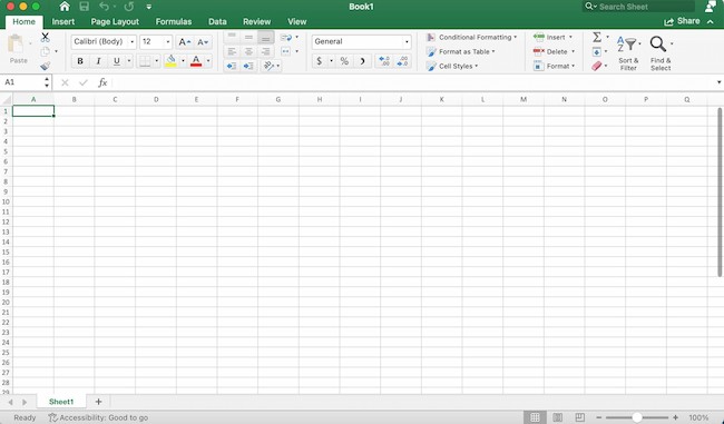
How to Download Microsoft Excel
It’s easy to download Microsoft Excel. First, check to make sure that your PC or Mac meets Microsoft’s system requirements. Next, sign in and install Microsoft 365.
After you sign in, follow the steps for your account and computer system to download and launch the program.
For example, say you’re working on a Mac desktop. You’ll click on Launchpad or look in your applications folder. Then, click on the Excel icon to open the application.
Microsoft Excel Spreadsheet Basics
Sometimes, Excel seems too good to be true. Need to combine data in multiple cells? Excel can do it. Need to copy formatting across an array of cells? Excel can do that, too.
Let’s start this Excel guide with the basics. Once you have these functions down, you’ll be ready to tackle more pro Excel tips and advanced lessons.
Inserting Rows or Columns
As you work with data, you might find yourself needing to add more rows and columns. Doing this one at a time would be super tedious. Luckily, there’s an easier way.
To add multiple rows or columns in a spreadsheet, highlight the number of pre-existing rows or columns that you want to add. Then, right-click and select «Insert.»
In this example, I add three rows to the top of my spreadsheet.
Autofill
Autofill lets you quickly fill adjacent cells with several types of data, including values, series, and formulas.
There are many ways to deploy this feature, but the fill handle is among the easiest.
First, choose the cells you want to be the source. Next, find the fill handle in the lower-right corner of the cell. Then either drag the fill handle to cover the cells you want to fill or just double-click.
Filters
When you’re looking at large data sets, you usually don’t need to look at every row at the same time. Sometimes, you only want to look at data that fit into certain criteria. That’s where filters come in.
Filters allow you to pare down data to only see certain rows at one time. In Excel, you can add a filter to each column in your data. From there, you can choose which cells you want to view.
To add a filter, click the Data tab and select «Filter.» Next, click the arrow next to the column headers. This lets you choose whether you want to organize your data in ascending or descending order, as well as which rows you want to show.
Let’s take a look at the Harry Potter example below. Say you only want to see the students in Gryffindor. By selecting the Gryffindor filter, the other rows disappear.
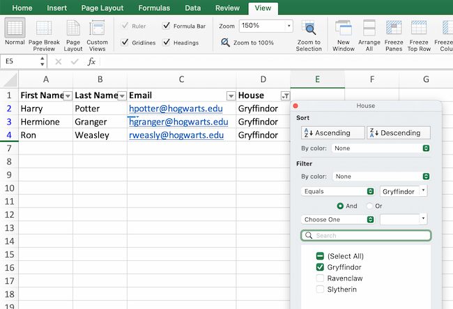
Pro tip: Start with a filtered view in your original spreadsheet. Then, copy and paste the values to another spreadsheet before you start analyzing.
Sort
Sometimes you’ll have a disorganized list of data. This is typical when you’re exporting lists, like marketing contacts or blog posts. Excel’s sort feature can help you alphabetize any list.
Click on the data in the column you want to sort. Then click on the «Data» tab in your toolbar and look for the «Sort» option on the left.
- If the «A» is on top of the «Z,» you can just click on that button once. Choosing A-Z means the list will sort in alphabetical order.
- If the «Z» is on top of the «A,» click the button twice. Z-A selection means the list will sort in reverse alphabetical order.
Remove Duplicates
Large datasets tend to have duplicate content. For example, you may have a list of different company contacts, but you only want to see the number of companies you have. In situations like this, removing duplicates comes in handy.
To remove duplicates, highlight the row or column where you noticed duplicate data. Then, go to the Data tab, and select «Remove Duplicates» (under Tools). A pop-up will appear so that you can confirm which data you want to keep. Select «Remove Duplicates,» and you’re good to go.
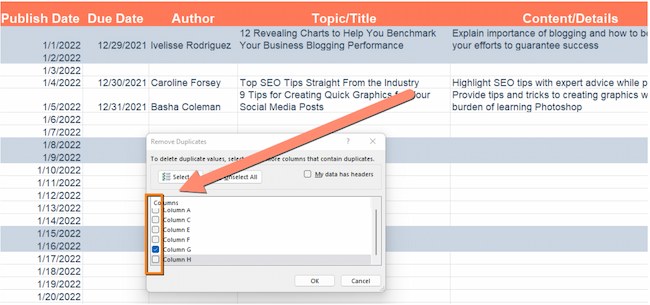
If you want to see an example, this post offers step-by-step instructions for removing duplicates.
You can also use this feature to remove an entire row based on a duplicate column value. So, say you have three rows of information and you only need to see one, you can select the whole dataset and then remove duplicates. The resulting list will have only unique data without any duplicates.
Paste Special
It’s often helpful to change the items in a row of data into a column (or vice versa). It would take a lot of time to copy and paste each individual header.
Not to mention, you may easily fall into one of the biggest, most unfortunate Excel traps — human error. Read here to check out some of the most common Microsoft Excel errors.
Instead of making one of these errors, let Excel do the work for you. Take a look at this example:
To use this function, highlight the column or row you want to transpose. Then, right-click and select «Copy.»
Next, select the cells where you want the first row or column to begin. Right-click on the cell, and then select «Paste Special.»
When the module appears, choose the option to transpose.
Paste Special is a super useful function. In the module, you can also choose between copying formulas, values, formats, or even column widths. This is especially helpful when it comes to copying the results of your pivot table into a chart.
Text to Columns
What if you want to split out information that’s in one cell into two different cells? For example, maybe you want to pull out someone’s company name through their email address. Or you want to separate someone’s full name into a first and last name for your email marketing templates.
Thanks to Microsoft Excel, both are possible. First, highlight the column where you want to split up. Next, go to the Data tab and select «Text to Columns.» A module will appear with more information. First, you need to select either «Delimited» or «Fixed Width.»
- Delimited means you want to break up the column based on characters such as commas, spaces, or tabs.
- Fixed Width means you want to select the exact location in all the columns where you want the split to occur.
Select «Delimited» to separate the full name into first name and last name.
Then, it’s time to choose the delimiters. This could be a tab, semicolon, comma, space, or something else. (For example, «something else» could be the «@» sign used in an email address.) Let’s choose the space for this example. Excel will then show you a preview of what your new columns will look like.
When you’re happy with the preview, press «Next.» This page will allow you to select Advanced Formats if you choose to. When you’re done, click «Finish.»
Format Painter
Excel has a lot of features to make crunching numbers and analyzing your data quick and easy. But if you ever spent some time formatting a spreadsheet, you know it can get a bit tedious.
Don’t waste time repeating the same formatting commands over and over again. Use the format painter to copy formatting from one area of the worksheet to another.
To do this, choose the cell you’d like to replicate. Then, select the format painter option (paintbrush icon) from the top toolbar. When you release the mouse, your cell should show the new format.
Keyboard Shortcuts
Creating reports in Excel is time-consuming enough. How can we spend less time navigating, formatting, and selecting items in our spreadsheet? Glad you asked. There are a ton of Excel shortcuts out there, including some of our favorites listed below.
Create a New Workbook
PC: Ctrl-N | Mac: Command-N
Select Entire Row
PC: Shift-Space | Mac: Shift-Space
Select Entire Column
PC: Ctrl-Space | Mac: Control-Space
Select Rest of Column
PC: Ctrl-Shift-Down/Up | Mac: Command-Shift-Down/Up
Select Rest of Row
PC: Ctrl-Shift-Right/Left | Mac: Command-Shift-Right/Left
Add Hyperlink
PC: Ctrl-K | Mac: Command-K
Open Format Cells Window
PC: Ctrl-1 | Mac: Command-1
Autosum Selected Cells
PC: Alt-= | Mac: Command-Shift-T
Excel Formulas
At this point, you’re getting used to Excel’s interface and flying through quick commands on your spreadsheets.
Now, let’s dig into the core use case for the software: Excel formulas. Excel can help you do simple arithmetic like adding, subtracting, multiplying, or dividing any data.
- To add, use the + sign.
- To subtract, use the — sign.
- To multiply, use the * sign.
- To divide, use the / sign.
- To use exponents, use the ^ sign.
Remember, all formulas in Excel must begin with an equal sign (=). Use parentheses to make sure certain calculations happen first. For example, consider how =10+10*10 is different from =(10+10)*10.
Besides manually typing in simple calculations, you can also refer to Excel’s built-in formulas. Some of the most common include:
- Average: =AVERAGE(cell range)
- Sum: =SUM(cell range)
- Count: =COUNT(cell range)
Also note that series’ of specific cells are separated by a comma (,), while cell ranges are notated with a colon (:). For example, you could use any of these formulas:
- =SUM(4,4)
- =SUM(A4,B4)
- =SUM(A4:B4)
Conditional Formatting
Conditional formatting lets you change a cell’s color based on the information within the cell. For example, say you want to flag a category in your spreadsheet.
To get started, highlight the group of cells you want to use conditional formatting on. Then, choose «Conditional Formatting» from the Home menu. Next, select a logic option from the dropdown. A window will pop up that prompts you to provide more information about your formatting rule. Select «OK» when you’re done, and you should see your results automatically appear.
Note: You can also create your own logic if you want something beyond the dropdown choices.
Dollar Signs
Have you ever seen a dollar sign in an Excel formula? When this symbol is in a formula, it isn’t representing an American dollar. Instead, it makes sure that the exact column and row stay the same even if you copy the same formula in adjacent rows.
You see, a cell reference — when you refer to cell A5 from cell C5, for example — is relative by default.
This means you’re actually referring to a cell that’s five columns to the left (C minus A) and in the same row (5). This is called a relative formula.
When you copy a relative formula from one cell to another, it’ll adjust the values in the formula based on where it’s moved. But sometimes, you want those values to stay the same no matter whether they’re moved around or not. You can do that by making the formula in the cell into what’s called an absolute formula.
To change the relative formula (=A5+C5) into an absolute formula, precede the row and column values with dollar signs, like this: (=$A$5+$C$5).
Combine Cells Using «&»
Databases tend to split out data to make it as exact as possible. For example, instead of having data that shows a person’s full name, a database might have the data as a first name and then a last name in separate columns.
In Excel, you can combine cells with different data into one cell by using the «&» sign in your function. The example below uses this formula: =A2&» «&B2.
Let’s go through the formula together using an example. So, let’s combine first names and last names into full names in a single column.
To do this, put your cursor in the blank cell where you want the full name to appear. Next, highlight one cell that contains a first name, type in an «&» sign, and then highlight a cell with the corresponding last name.
But you’re not finished. If all you type in is =A2&B2, then there will not be a space between the person’s first name and last name. To add that necessary space, use the function =A2&» «&B2. The quotation marks around the space tell Excel to put a space between the first and last name.
To make this true for multiple rows, drag the corner of that first cell downward as shown in the example.
Pivot Tables
Pivot tables reorganize data in a spreadsheet. A pivot table won’t change the data that you have, but it can sum up values and compare information in a way that’s easy to understand.
For example, let’s look at how many people are in each house at Hogwarts.
To create the Pivot Table, go to Insert > Pivot Table. Excel will automatically populate your pivot table, but you can always change the order of the data. Then, you have four options to choose from.
Report Filter
This allows you to only look at certain rows in your dataset.
For example, to create a filter by house, choose only students in Gryffindor.
Column and Row Labels
These could be any headers or rows in the dataset.
Note: Both Row and Column labels can contain data from your columns. For example, you can drag First Name to either the Row or Column label depending on how you want to see the data.
Value
This section allows you to convert data into a number. Instead of just pulling in any numeric value, you can sum, count, average, max, min, count numbers, or do a few other manipulations with your data. By default, when you drag a field to Value, it always does a count.
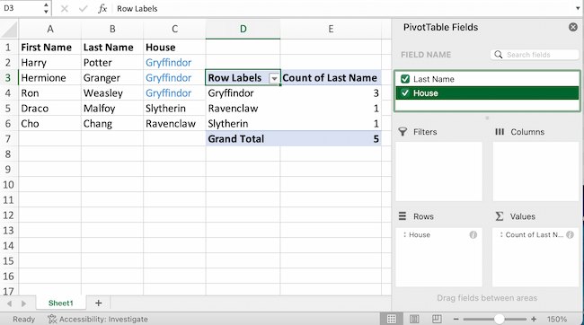
The example above counts the number of students in each house. To recreate this pivot table, go to the pivot table and drag the House column to both the row Labels and the values. This will sum up the number of students associated with each house.
IF Functions
At its most basic level, Excel’s IF function lets you see if a condition you set is true or false for a given value.
If the condition is true, you get one result. If the condition is false, you get another result.
This popular tool is useful for comparisons and finding errors. But if you’re new to Excel you may need a little more information to get the most out of this feature.
Let’s take a look at this function’s syntax:
- =IF(logical_test, value_if_true, [value_if_false])
- With values, this could be: =IF(A2>B2, «Over Budget», «OK»)
In this example, you want to find where you’re overspending. With this IF function, if your spending (what’s in A2) is greater than your budget (what’s in B2), that overspending will be easy to see. Then you can then filter the data so that you see only the line items where you’re going over budget.
The real power of the IF function comes when you string or «nest» multiple IF statements together. This allows you to set multiple conditions, get more specific results, and organize your data into more manageable chunks.
For example, ranges are one way to segment your data for better analysis. For example, you can categorize data into values that are less than 10, 11 to 50, or 51 to 100.
- =IF(B3<11,»10 or less»,IF(B3<51,»11 to 50″,IF(B3<100,»51 to 100″)))
Let’s talk about a few more IF functions.
COUNTIF Function
The power of IF functions goes beyond simple true and false statements. With the COUNTIF function, Excel can count the number of times a word or number appears in any range of cells.
For example, let’s say you want to count the number of times the word «Gryffindor» appears in this data set.
Take a look at the syntax.
- The formula: =COUNTIF(range, criteria)
- The formula with variables from the example below: =COUNTIF(D:D,»Gryffindor»)
In this formula, there are several variables:
Range
The range that you want the formula to cover.
In this one-column example, «D:D» shows that the first and last columns are both D. If you want to look at columns C and D, use «C:D.»
Criteria
Whatever number or piece of text you want Excel to count.
Only use quotation marks if you want the result to be text instead of a number. In this example, «Gryffindor» is the only criteria.
To use this function, type the COUNTIF formula in any cell and press «Enter.» Using the example above, this action will show how many times the word «Gryffindor» appears in the dataset.
SUMIF Function
Ready to make the IF function a bit more complex? Let’s say you want to analyze the number of leads your blog has generated from one author, not the entire team.
With the SUMIFS function, you can add up cells that meet certain criteria. You can add as many different criteria to the formula as you like.
Here’s your formula:
- =SUMIFS(sum_range, criteria_range1, criteria1, [criteria_range2, criteria 2],etc.)
That’s a lot of criteria. Let’s take a look at each part:
Sum_range
The range of cells you’re going to add up.
Criteria_range1
The range that is being searched for your first value.
Criteria1
This is the specific value that determines which cells in Criteria_range1 to add together.
Note: Remember to use quotation marks if you’re searching for text.
In the example below, the SUMIF formula counts the total number of house points from Gryffindor.

If AND/OR
The OR and AND functions round out your IF function choices. These functions check multiple arguments. It returns either TRUE or FALSE depending on if at least one of the arguments is true (this is the OR function), or if all of them are true (this is the AND function).
Lost in a sea of «and’s» and «or’s»? Don’t check out yet. In practice, OR and AND functions will never be used on their own. They need to be nested inside of another IF function. Recall the syntax of a basic IF function:
- =IF(logical_test, value_if_true, [value_if_false])
- Now, let’s fit an OR function inside of the logical_test: =IF(OR(logical1, logical2), value_if_true, [value_if_false])
To put it plainly, this combined formula allows you to return a value if both conditions are true, as opposed to just one. With AND/OR functions, your formulas can be as simple or complex as you want them to be, as long as you understand the basics of the IF function.
VLOOKUP
Have you ever had two sets of data on two different spreadsheets that you want to combine into a single spreadsheet?
For example, say you have a list of names and email addresses in one spreadsheet and a list of email addresses and company names in a different spreadsheet. But you want the names, email addresses, and company names of those people to appear in one spreadsheet.
VLOOKUP is a great go-to formula for this.
Before you use the formula, be sure that you have at least one column that appears identically in both places.
Note: Scour your data sets to make sure the column of data you’re using to combine spreadsheets is exactly the same. This includes removing any extra spaces.
In the example below, Sheet One and Sheet Two are both lists with different information about the same people. The common thread between the two is their email addresses. Let’s combine both datasets so that all the house information from Sheet Two translates over to Sheet One.
Type in the formula: =VLOOKUP(C2,Sheet2!A:B,2,FALSE). This will bring all the house data into Sheet One.
Now that you’ve seen how VLOOKUP works, let’s review the formula.
- The formula: =VLOOKUP(lookup value, table array, column number, [range lookup])
- The formula with variables from the example: =VLOOKUP(C2,Sheet2!A:B,2,FALSE)
In this formula, there are several variables.
Lookup Value
A value that LOOKUP searches for in an array. So, your lookup value is the identical value you have in both spreadsheets.
In the example, the lookup value is the first email address on the list, or cell 2 (C2).
Table Array
Table arrays hold column-oriented or tabular data, like the columns on Sheet Two you’re going to pull your data from.
This table array includes the column of data identical to your lookup value in Sheet One and the column of data you’re trying to copy to Sheet Two.
In the example, «A» means Column A in Sheet Two. The «B» means Column B.
So, the table array is «Sheet2!A:B.»
Column Number
Excel refers to columns as letters and rows as numbers. So, the column number is the selected column for the new data you want to copy.
In the example, this would be the «House» column. «House» is column 2 in the table array.
Note: Your range can be more than two columns. For example, if there are three columns on Sheet Two — Email, Age, and House — and you also want to bring House onto Sheet One, you can still use a VLOOKUP. You just need to change the «2» to a «3» so it pulls back the value in the third column. The formula for this would be: =VLOOKUP(C2:Sheet2!A:C,3,false).]
Range Lookup
This term means that you’re looking for a value within a range of values. You can also use the term «FALSE» to pull only exact value matches.
Note: VLOOKUP will only pull back values to the right of the column containing your identical data on the second sheet. This is why some people prefer to use the INDEX and MATCH functions instead.
INDEX MATCH
Like VLOOKUP, the INDEX and MATCH functions pull data from another dataset into one central location. Here are the main differences:
VLOOKUP is a much simpler formula.
If you’re working with large datasets that need thousands of lookups, the INDEX MATCH function will decrease load time in Excel.
INDEX MATCH formulas work right-to-left.
VLOOKUP formulas only work as a left-to-right lookup. So, if you need to do a lookup that has a column to the right of the results column, you’d have to rearrange those columns to do a VLOOKUP. This can be tedious with large datasets and lead to errors.
Let’s look at an example. Let’s say Sheet One contains a list of names and their Hogwarts email addresses. Sheet Two contains a list of email addresses and each student’s Patronus.
The information that lives in both sheets is the email addresses column. But, the column numbers for email addresses are different on the two sheets. So, you’d use the INDEX MATCH formula instead of VLOOKUP to avoid column-switching errors.
The INDEX MATCH formula is the MATCH formula nested inside the INDEX formula.
- The formula: =INDEX(table array, MATCH formula)
- This becomes: =INDEX(table array, MATCH (lookup_value, lookup_array))
- The formula with variables from the example: =INDEX(Sheet2!A:A,(MATCH(Sheet1!C:C,Sheet2!C:C,0)))
Here are the variables:
Table Array
The range of columns on Sheet Two that contain the new data you want to bring over to Sheet One.
In the example, «A» means Column A, and has the «Patronus» information for each person.
Lookup Value
This Sheet One column has identical values in both spreadsheets.
In the example, this is the «email» column on Sheet One, which is Column C. So, Sheet1!C:C.
Lookup Array
Again, an array is a group of values in rows and columns that you want to search.
In this example, the lookup array is the column in Sheet Two that contains identical values in both spreadsheets. So, the «email» column on Sheet Two, Sheet2!C:C.
Once you have your variables set, type in the INDEX MATCH formula. Add it where you want the combined information to populate.
Data Visualization
Now that you’ve learned formulas and functions, let’s make your analysis visual. With a beautiful graph, your audience will be able to process and remember your data more easily.
Create a Basic Graph
First, decide what type of graph to use. Bar charts and pie charts help you compare categories. Pie charts compare part of a whole and are often best when one of the categories is way larger than the others. Bar charts highlight incremental differences between categories. Finally, line charts can help display trends over time.
This post can help you find the best chart or graph for your presentation.
Next, highlight the data you want to turn into a chart. Then choose «Charts» in the top navigation. You can also use Insert > Chart if you have an older version of Excel. Then you can adjust and resize your chart until it makes the statement you’re hoping for.
Microsoft Excel Can Help Your Business Grow
Excel is a useful tool for any small business. Whether you’re focused on marketing, HR, sales, or service, these Microsoft Excel tips can boost your performance.
Whether you want to improve efficiency or productivity, Excel can help. You can find new trends and organize your data into usable insights. It can make your data analysis easier to understand and your daily tasks easier.
All it takes is a little know-how and some time with the software. So start learning, and get ready to grow.
Editor’s note: This post was originally published in April 2018 and has been updated for comprehensiveness.
