
Freeze panes to lock rows and columns
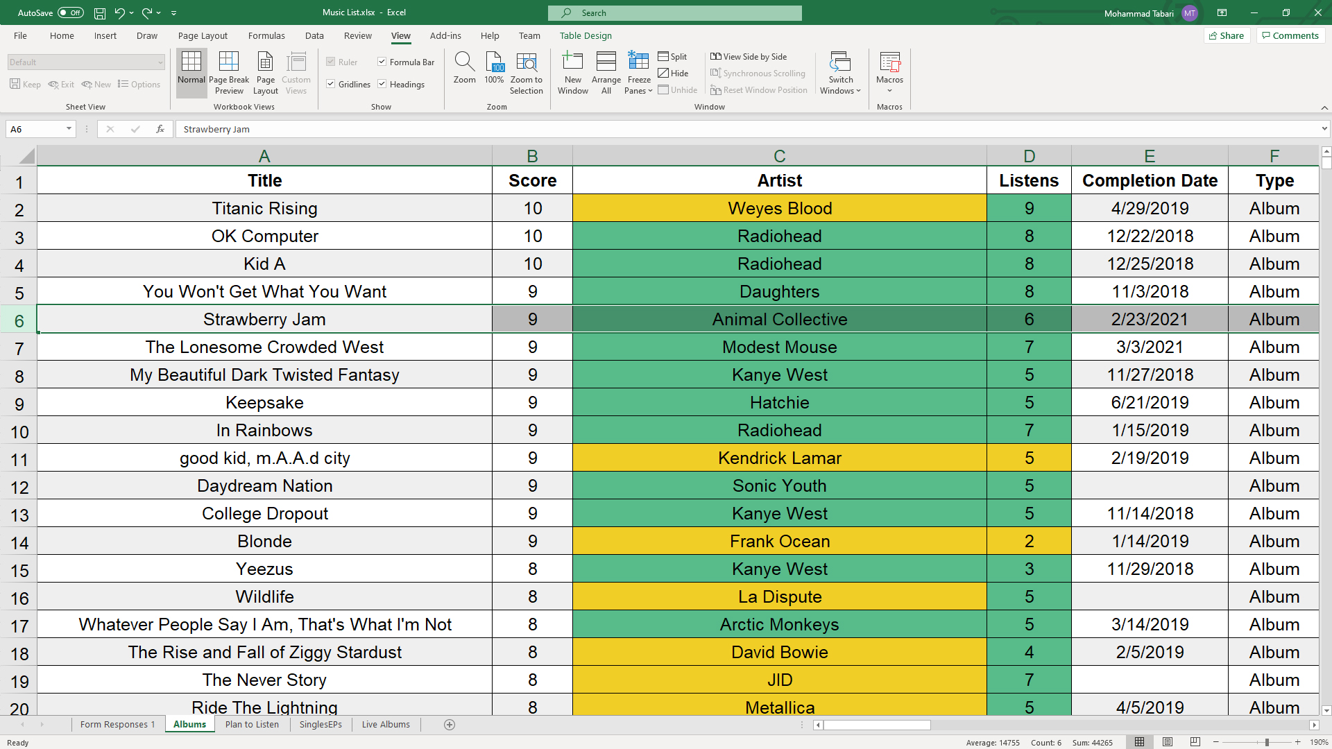
To keep an area of a worksheet visible while you scroll to another area of the worksheet, go to the View tab, where you can Freeze Panes to lock specific rows and columns in place, or you can Split panes to create separate windows of the same worksheet.

Freeze rows or columns
Freeze the first column
-
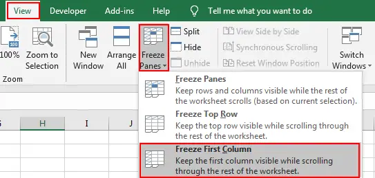
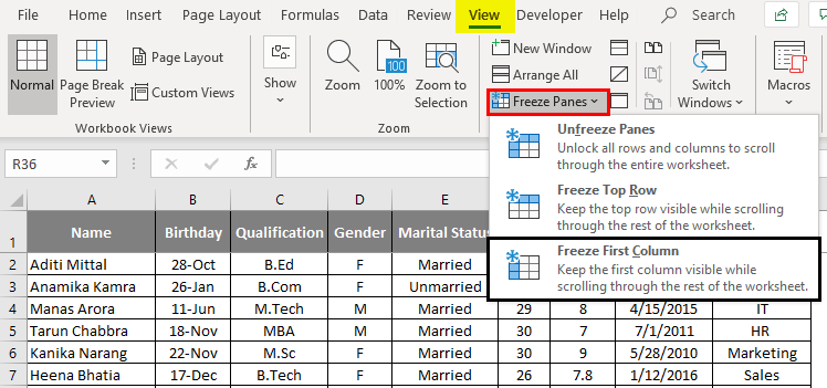
Select View > Freeze Panes > Freeze First Column.
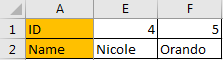
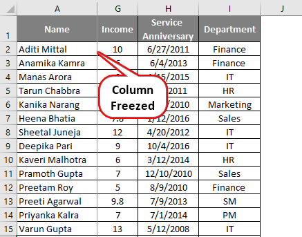
The faint line that appears between Column A and B shows that the first column is frozen.
Freeze the first two columns
-
Select the third column.
-
Select View > Freeze Panes > Freeze Panes.
Freeze columns and rows
-
Select the cell below the rows and to the right of the columns you want to keep visible when you scroll.
-
Select View > Freeze Panes > Freeze Panes.
Unfreeze rows or columns
-
On the View tab > Window > Unfreeze Panes.

Note: If you don’t see the View tab, it’s likely that you are using Excel Starter. Not all features are supported in Excel Starter.
Need more help?
You can always ask an expert in the Excel Tech Community or get support in the Answers community.
See Also
Freeze panes to lock the first row or column in Excel 2016 for Mac
Split panes to lock rows or columns in separate worksheet areas
Overview of formulas in Excel
How to avoid broken formulas
Find and correct errors in formulas
Keyboard shortcuts in Excel
Excel functions (alphabetical)
Excel functions (by category)
Need more help?
Freezing columns in excel fixes or locks them so that they remain visible while scrolling through the database. A frozen column does not move with the movement of the remaining columns.
For example, freezing the first column (column A) ensures that it stays at its place at the time of navigation through the rest of the columns. Moreover, if column A consists of headings, the user may want to view these while working on the other columns of the dataset.
The objectives of freezing an excel column are:
- To ensure that the user does not lose track of the specific column
- To facilitate comparison of different columns of the worksheet
Freezing columns prevents the user from referring to the same column again and again. In other words, the frozen columns save the scrolling time of the user.
All the properties of the frozen column apply to the frozen row as well.
The “freeze panesFreezing panes in excel helps freeze one or more rows and/or columns so that they remain fixed while scrolling through the database.read more” drop-down under the View tab lists the following options:
- Freeze panes–It freezes multiple rows and columns.
- Freeze top row–It freezes only the first row.
- Freeze first column–It freezes only the first column.
After freezing a row or column in excel, a grey line appears at the end of the frozen area. This line indicates that the row or column has been frozen.
Table of contents
- #1 Freeze the First Column in Excel
- Example #1
- #2 Freeze Multiple Columns in Excel
- Example #2
- #3 Freeze the Row and Column Together in Excel
- Example #3
- #4 Unfreeze Panes in Excel
- The Rules of Freezing in Excel
- Frequently Asked Questions
- Recommended Articles
Let us go through the ways of freezing the first excel column, multiple columns, and both rows and columns.
#1 Freeze the First Column in Excel
Freezing the first column locks column A of the worksheet. This means that on moving from left to right, this column will be visible at all times.
In addition, column A is fixed irrespective of the column from which the actual data begins. The excel shortcut to freeze the first column is “Alt+W+F+C” (when pressed one by one).

Let us consider an example.
Example #1
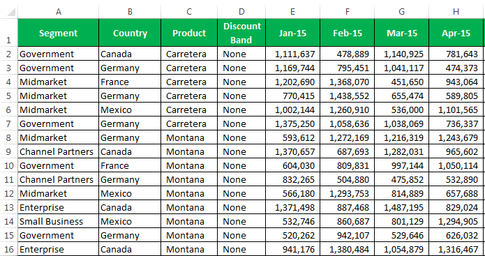
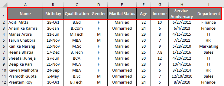
The following table shows the sales revenue (in $) generated by the products of specific segments. The data relates to various countries and is spread across the first five months of the year 2015.
We want to freeze the first excel column (column A).
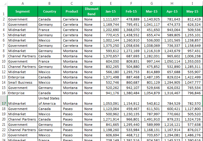
In order to view the column “segment” on a movement from left to right, we need to freeze it.
The steps for freezing the excel column are listed as follows:
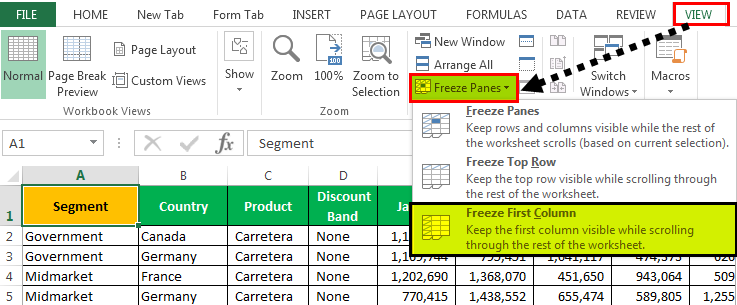
- Select the worksheet where the first column is to be frozen.
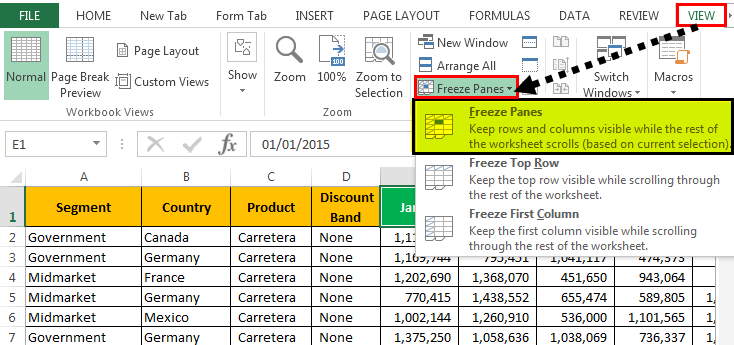
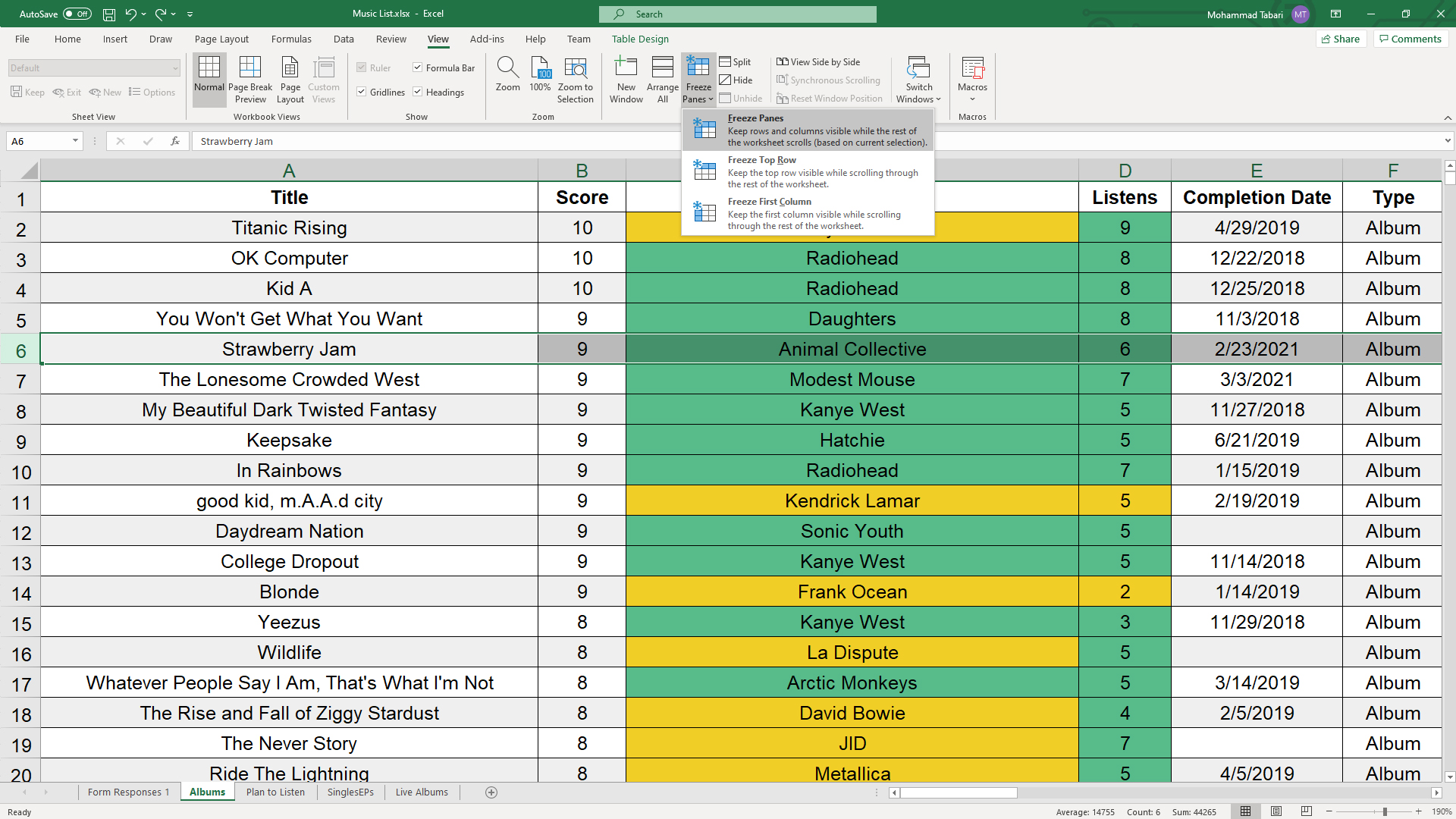
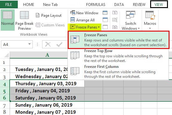
- In the View tab, click the “freeze panes” drop-down under the “window” section. Select “freeze first column,” as shown in the succeeding image.
Alternatively, press the shortcut keys “Alt+W+F+C” one by one.

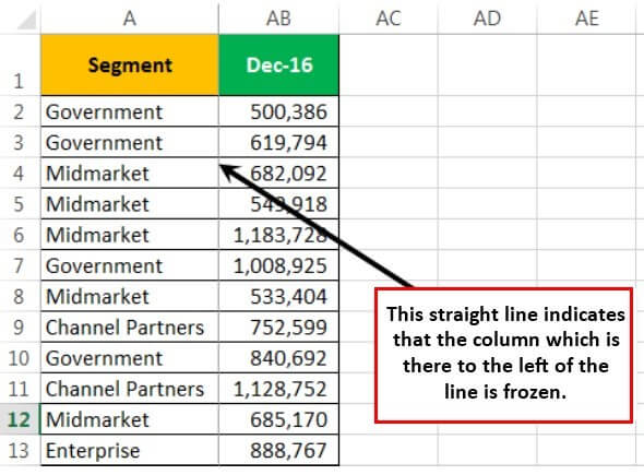
- The first column is frozen. The grey line appears at the end of column A indicating that the column to the left is frozen. The column AB shown in the following image is the last scrolled column of the dataset.

- On scrolling (from left to right) through the remaining columns of the dataset, column A is visible. The same is shown in the following image.

In the same way, the first row can be frozen.
#2 Freeze Multiple Columns in Excel
Freezing multiple excel columns is similar to freezing multiple rows. For freezing multiple columns, select the first right-hand side cell immediately after the last column to be frozen. This is because multiple columns are frozen based on the current selection.
Similarly, for freezing multiple rows, select the first cell immediately below the last row to be frozen.
For example, to freeze the columns A, B, and C, select the cell D1. By freezing the first three columns, they remain visible to the user at all times. Likewise, to freeze the rows 1, 2, and 3, select the cell A4.
The shortcut to freeze multiple excel columns is “Alt+W+F+F” (when pressed one by one).

Let us consider an example.
Example #2
Working on the data of example #1, we want to freeze the first four columns, A, B, C, and D.
The steps for freezing multiple excel columns are listed as follows:
Step 1: Select the cell E1. This is because the first four columns are to be frozen.
Step 2: In the View tab, click the “freeze panes” drop-down under the “window” section. Select “freeze panes,” as shown in the succeeding image.
Alternatively, press the shortcut keys “Alt+W+F+F” one by one.
Step 3: The first four columns are frozen. The grey line appears (shown in the following image) at the end of column D, indicating that the columns to the left are frozen.
The columns R and S shown in the following image are the scrolled columns towards the end of the dataset.
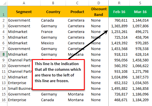
Step 4: On scrolling (from left to right) till the last column of the dataset, the first four columns are visible. The same is shown in the following image.
#3 Freeze the Row and Column Together in Excel
Usually, the first row and the first column of a database contain headers. The user might want to view the row 1 and the column A simultaneously and at all times. Hence, it is essential to lock them together to permit their visibility while scrolling down and from left to right.
The only difference between the methods #2 and #3 is in the selection of the cell (step 1). With the “freeze panes” option, Excel freezes the rows and columns preceding the current active cell.
The shortcut to freeze the row and column together is “Alt+W+F+F” (when pressed one by one).
Let us consider an example.
Example #3
Working on the data of example #1, we want to freeze the first row (row 1) and the first column (column A) at the same time.
The steps to freeze the excel row 1 and column A together are listed as follows:
Step 1: Select the cell B2.
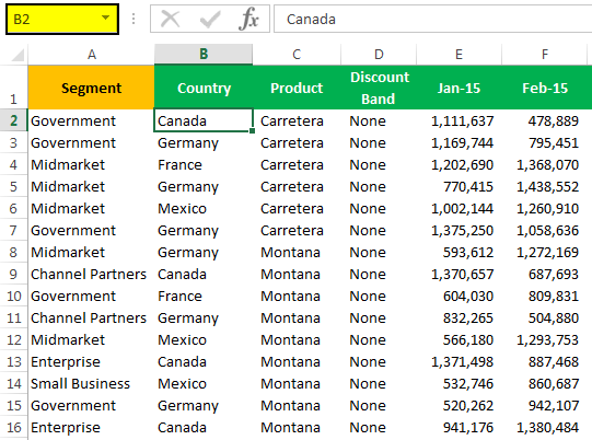
Step 2: Press the shortcut keys “Alt+W+F+F” one by one. It freezes the column to the left of the selected cell B2. At the same time, the row preceding the active cell (B2) is also frozen, as shown in the following image.
Hence two grey lines appear, one at the end of row 1 (horizontal) and the other at the end of column A (vertical).
Note: Alternatively, the “freeze panes” option can be selected from the “freeze panes” drop-down of the View tab.
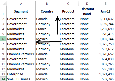
Step 3: On scrolling from top to bottom and left to right, the row 1 and column A are visible. The same is shown in the following image.
Note: It is possible to freeze as many rows and columns depending on the requirement. The condition is that freezing of multiple excel rows and columns should begin with the top row (row 1) and the first column (column A).
#4 Unfreeze Panes in Excel
Unfreezing of panes does not require any cells to be selected. The steps to unfreeze panes in Excel are listed as follows:
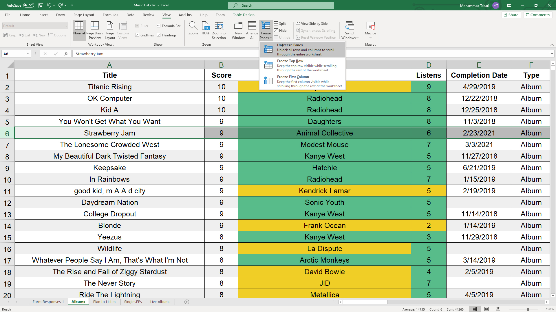
Step 1: In the View tab, click the “freeze panes” drop-down under the “window” section. Select “unfreeze panes,” as shown in the succeeding image.
Alternatively, press the shortcut keys “Alt+W+F+F” one by one.
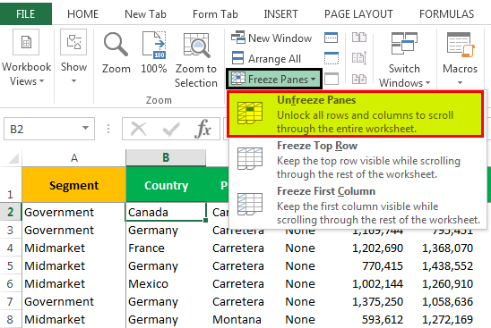
Step 2: The grey lines are removed, as shown in the following image.
Note: The “unfreeze panes” option appears only after freezes have been applied to the Excel worksheet.
The Rules of Freezing in Excel
The norms governing the freezing of rows and columns are listed as follows:
- It is not possible to freeze excel rows and columns in the middle of the worksheet.
- The option “freeze panes” can be applied only once. It is not possible to create multiple “freeze panes” in a single worksheet.
- The rows and columns to be fixed should be visible at the time of freezing. Otherwise, they will remain hidden even after freezing.
Note 1: To divide a worksheet into two or more areas with separate scroll barsIn Excel, there are two scroll bars: one is a vertical scroll bar that is used to view data from up and down, and the other is a horizontal scroll bar that is used to view data from left to right.read more for each, use the “split” option. This is available in the “window” section of the View tab.
Note 2: To fix the header row of a large dataset that does not fit into the screen, create an Excel tableIn excel, tables are a range with data in rows and columns, and they expand when new data is inserted in the range in any new row or column in the table. To use a table, click on the table and select the data range.read more. Moreover, ensure the visibility of this row by selecting any cell within the table before scrolling.
Frequently Asked Questions
1. What does freezing columns mean and how to freeze the first column in Excel?
Freezing a column means locking it in order to keep it visible while the user scrolls through the database. This is specifically helpful if a column contains headers which are required to be seen at all times.
After freezing, a grey line appears to indicate the frozen columns on its left. The steps to freeze the first column (column A) are listed as follows:
• In the View tab, click the “freeze panes” drop-down under the “window” section.
• Select “freeze first column.” Alternatively, press the shortcut keys “Alt+W+F+C” one by one.
• The first column (column A) is frozen.
Note: For freezing the first row, select “freeze top row” from the “freeze panes” drop-down of the View tab.
2. How to freeze multiple columns in Excel?
Let us freeze columns A, B, C, D, and E. The steps to freeze multiple columns in Excel are listed as follows:
• Select either the column or the first cell to the right of the last column to be frozen (column E). So, select either column F or the cell F1.
• In the View tab, click the “freeze panes” drop-down under the “window” section.
• Select “freeze panes.” Alternatively, press the shortcut keys “Alt+W+F+F” one by one.
• The columns A B, C, D, and E are frozen as indicated by the grey line at the end of column E.
3. How to freeze rows and columns together in Excel?
Let us freeze rows 1, 2, and 3 and columns A, B, and C. The steps to freeze the given rows and columns together are listed as follows:
• Select cell D4 based on the following parameters:
a. It immediately follows the last row to be frozen (row 3).
b. It is to the right of the last column to be frozen (column C).
• In the View tab, click the “freeze panes” drop-down under the “window” section.
• Select “freeze panes.” Alternatively, press the shortcut keys “Alt+W+F+F” one by one.
• The rows 1, 2, and 3 and columns A, B, and C are frozen. This is indicated by the grey line appearing below row 3 and at the end of column C.
Note: The freezing of multiple excel rows and columns should begin with the top row (row 1) and the first column (column A).
Recommended Articles
This has been a guide to freezing columns in Excel. Here we discuss how to freeze the first column, multiple columns, and both rows and columns. For more on Excel, take a look at the following articles-
- Adding Columns in ExcelAdding a column in excel means inserting a new column to the existing dataset.read more
- Group Excel ColumnsIn Excel, grouping one or more columns together in a worksheet is referred to as group column and I t allows you to contract or expand the column.read more
- Column Lock in ExcelThe Column Lock feature in Excel is designed to prevent any mishaps or unwanted modifications in data caused by a user’s mistake. It may be used on single or multiple columns, with cell formatting ranging from locked to unlocked, and the workbook can be password protected.read more
- Column Sort in Excel
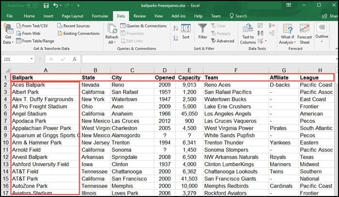
If you work with large spreadsheets, you often need to scroll down or right quite frequently, looking for information. However, this means moving away from the information you need to keep an eye on. The first row usually contains the column headers or field labels, while the first column tends to contain identifying information for the row or record. Fortunately, you can easily freeze rows, columns, and panes in Microsoft Excel, so you can always keep the information you need in sight.
In this guide, you will learn how to freeze rows, columns, and panes in Microsoft Excel. You will learn how to freeze the top row or the first column from the ‘View’ menu. You will also learn how to freeze panes, which can combine rows and columns. You have step-by-step instructions on how to use the ‘Freeze Panes’ options to freeze both rows and columns, only rows, or only columns. Finally, you will learn how to unfreeze rows, columns, and panes in Google Sheets.
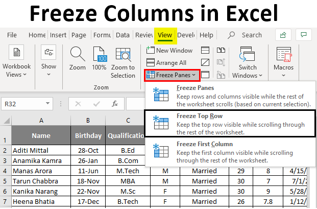
How to Freeze the Top Row in Excel?
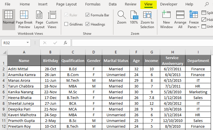
Freezing the top row of the current sheet in Excel is very easy. Go to the View tab and click “Freeze Top Row”.

How to Freeze a Row or Column in Excel — View > Freeze Top Row
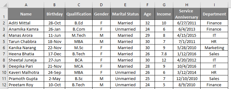
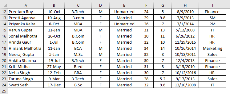
That’s it. You can now scroll as far down as you want without losing track of the information in the first row.

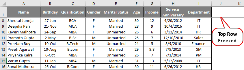
How to Freeze a Row or Column in Excel — Top Row Frozen
How to Freeze the First Column in Excel?
Freezing the top column is just as easy as freezing the top row. On the ‘View’ tab, click ‘Freeze First Column”

How to Freeze a Row or Column in Excel — View > Freeze First Column
That’s it. You can now scroll as far right as you want without losing track of the information in the first column.

How to Freeze a Row or Column in Excel — First Column Frozen
How to Freeze Panes in Excel?
Think of it as selecting the first cell that you don’t want to freeze. Excel will freeze anything above or to the left of the cell you select. This means you can freeze the top row and first column simultaneously. In fact, you can choose to freeze a different number of rows and columns, as well as only freeze multiple rows or multiple columns only.
Freeze Top Row & First Column
As mentioned above, when using the pane option, Excel will freeze anything above and to the left of the cell you select. If you want to freeze the top row and first column, select cell B2 and click ‘Freeze Pane’.

How to Freeze a Row or Column in Excel — Freeze Pane
As you can see below, row 1 and column A are now frozen in place, no matter how far down or right you scroll.

How to Freeze a Row or Column in Excel — Top Row & First Column Frozen
Freeze Multiple Rows & Columns
Sometimes, tables are not placed neatly on the top left corner of the spreadsheet, and they’re not yours to move. However, you still want to be able to freeze the headers and the first column with data. The option to ‘Freeze Panes’ is very flexible, so you can do this easily.
Just remember to select the first cell you don’t want to freeze, as Excel will freeze anything to the left or above your selection when you click ‘Freeze Pane’ in the ‘View’ tab.

How to Freeze a Row or Column in Excel — Freeze Multiple Rows & Columns
That’s it. Multiple rows and columns are now frozen, so you can move around your table while keeping an eye on the information you need.

How to Freeze a Row or Column in Excel — Frozen Pane
Freeze Multiple Rows
To freeze multiple rows only, select a cell in the first column in the row below the last one you want to freeze.

How to Freeze a Row or Column in Excel — Select Cell
The rows above the selected cell are now frozen.

How to Freeze a Row or Column in Excel — Multiple Rows Frozen
Freeze Multiple Columns
To freeze multiple columns only, select a cell in the first row in the column to the right of the last one you want to freeze.

How to Freeze a Row or Column in Excel — Select Cell
The columns to the left of the selected cell are now frozen.

How to Freeze a Row or Column in Excel — Multiple Columns Frozen
How to Unfreeze Rows, Columns, and Panes in Excel?
Fortunately, unfreezing rows, columns, or panes is even easier than freezing them.
Go to the ‘View’ tab and click ‘Unfreeze Panes’, and this will instantly unfreeze any frozen rows and columns.

How to Freeze a Row or Column in Excel — Unfreeze Panes
If the ‘Unfreeze Panes” is not available, it means there are no frozen rows or panes in that sheet.

How to Freeze a Row or Column in Excel — No Frozen Rows or Columns
Want to Boost Your Team’s Productivity and Efficiency?
Transform the way your team collaborates with Confluence, a remote-friendly workspace designed to bring knowledge and collaboration together. Say goodbye to scattered information and disjointed communication, and embrace a platform that empowers your team to accomplish more, together.
Key Features and Benefits:
- Centralized Knowledge: Access your team’s collective wisdom with ease.
- Collaborative Workspace: Foster engagement with flexible project tools.
- Seamless Communication: Connect your entire organization effortlessly.
- Preserve Ideas: Capture insights without losing them in chats or notifications.
- Comprehensive Platform: Manage all content in one organized location.
- Open Teamwork: Empower employees to contribute, share, and grow.
- Superior Integrations: Sync with tools like Slack, Jira, Trello, and more.
Limited-Time Offer: Sign up for Confluence today and claim your forever-free plan, revolutionizing your team’s collaboration experience.
Conclusion
Freezing rows and columns is easy in Microsoft Excel. In the ‘View’ tab, there are two buttons to instantly freeze the top row or the first column without even having to select them first. However, there are times when you need to freeze multiple rows or columns or even both at the same time.
Fortunately, there is another button that allows you to freeze as many rows and columns as you want: ‘Freeze Panes’. Just select the cell below the row you want to freeze, and to the right of the column you want to freeze, then click ‘Freeze Panes’. Finally, you also know that you can instantly unfreeze any frozen rows, columns, or panes in your sheet by clicking a single button: ‘Unfreeze Panes’.
To learn how to freeze rows and columns in Google Sheets, as well as other Microsoft Excel and Google Sheets topics, check out our guides on:
- How to Freeze a Row or Column in Google Sheets
- How to Unhide Excel Sheets and How to Hide Sheets in Excel
- How To Hide And Unhide Tabs In Google Sheets
- How to Lock Cells in Excel (Cells, Sheets & Formulas)
- How to Unlock Cells in Excel
- How to Combine Multiple Excel Columns Into One
- How to Merge Cells in Google Sheets (Complete Guide)
![]()
Download Article
![]()
Download Article
- Freezing the First Column or Row
- Freezing Multiple Columns or Rows
- Video
- Q&A
|
|
|
This wikiHow teaches you how to freeze specific rows and columns in your Microsoft Excel worksheet. Freezing rows or columns ensures that certain cells remain visible as you scroll through the data. If you want to easily edit two parts of the spreadsheet at once, splitting your panes will make the task much easier.
-
1
Click the View tab. It’s at the top of Excel. Frozen cells are rows or columns that remain visible while you scroll through a worksheet.[1]
If you want column headers or row labels to remain visible as you work with large amounts of data, you’ll likely find it helpful to lock those cells into place.- Only whole rows or columns can be frozen. It is not possible to freeze individual cells.
-
2
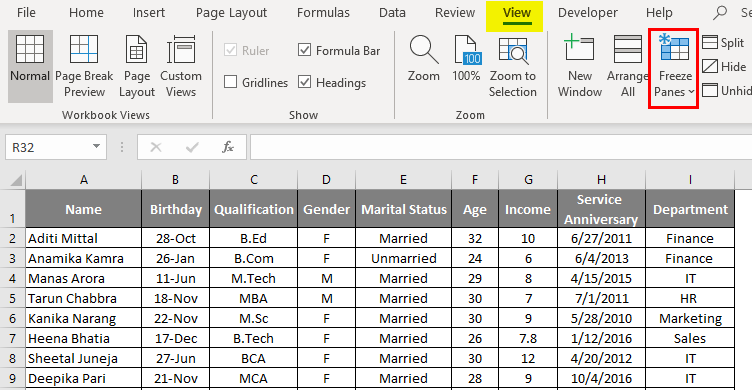
Click the Freeze Panes button. It’s in the «Window» section of the toolbar. A set of three freezing options will appear.
Advertisement
-
3
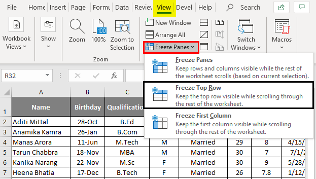
Click Freeze Top Row or Freeze First Column. If you want to keep the top row of cells in place as you scroll down through your data, select Freeze Top Row. To keep the first column in place as you scroll horizontally, select Freeze First Column.
-
4
Unfreeze your cells. If you want to unlock the frozen cells, click the Freeze Panes menu again and select Unfreeze Panes.


Advertisement
-
1
Select the row or column after those you want to freeze. If the data you want to keep stationary takes up more than one row or column, click the column letter or row number after those you want to freeze. For example:
- If you want to keep rows 1, 2, and 3 in place as you scroll down through your data, click row 4 to select it.
- If you want columns A and B to remain still as you scroll sideways through your data, click column C to select it.
- Frozen cells must connect to the top or left edge of the spreadsheet. It’s not possible to freeze rows or columns in the middle of the sheet.[2]
-
2
Click the View tab. It’s at the top of Excel.
-
3
Click the Freeze Panes button. It’s in the «Window» section of the toolbar. A set of three freezing options will appear.
-
4
Click Freeze Panes on the menu. It’s at the top of the menu. This freezes the columns or rows before the one you selected.
-
5
Unfreeze your cells. If you want to unlock the frozen cells, click the Freeze Panes menu again and select Unfreeze Panes.


Advertisement
Add New Question
-
Question
How do I freeze the top two rows?

Select the row directly under the rows you want to freeze (in this case, the third row). Go to View, Freeze Panes, and select «Freeze Panes.» Everything above the row you have selected will be frozen.
Ask a Question
200 characters left
Include your email address to get a message when this question is answered.
Submit
Advertisement
Thanks for submitting a tip for review!
wikiHow Video: How to Freeze Cells in Excel
About This Article
Article SummaryX
1. Click View.
2. Click Freeze Panes.
3. Select Freeze Top Row or Freeze First Column.
Did this summary help you?
Thanks to all authors for creating a page that has been read 171,421 times.
Is this article up to date?
When you’re working with a lot of spreadsheet data on your laptop, keeping track of everything can be difficult. It’s one thing to compare one or two rows of information when dealing with a small subset of data, but when a dozen rows are involved, things get unwieldy. And we haven’t even started talking about columns yet. When your spreadsheets become unmanageable, there’s only one solution: freeze the rows and columns.
Freezing rows and columns in Excel makes navigating your spreadsheet much easier. When done correctly, the chosen panes are locked in place; this means those specific rows are always visible, no matter how far you scroll down. More often than not, you’ll only freeze a couple of rows or a column, but Excel doesn’t limit how many of either you can freeze, which can come in handy for larger sheets.
This how-to works with Microsoft Excel 2016 as well as later versions. However, the this method also works with Google Sheets, OpenOffice and LibreOffice. Ready to get to work? Here’s how to freeze rows and columns in Excel:
- More: How to put Windows 10 into Safe Mode
- Here’s how to lock cells in Excel and how to recover a deleted or unsaved file in Excel
- This is how to use VLOOKUP in Excel and add additional rows above or below in Excel
How to freeze a row in Excel
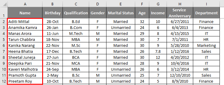
1. Select the row right below the row or rows you want to freeze. If you want to freeze columns, select the cell immediately to the right of the column you want to freeze. In this example, we want to freeze rows 1 to 5, so we’ve selected row 6.
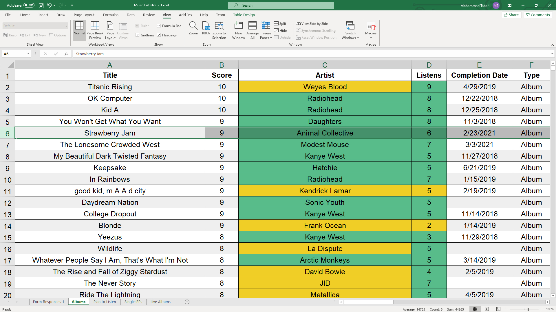
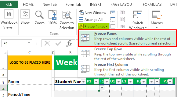
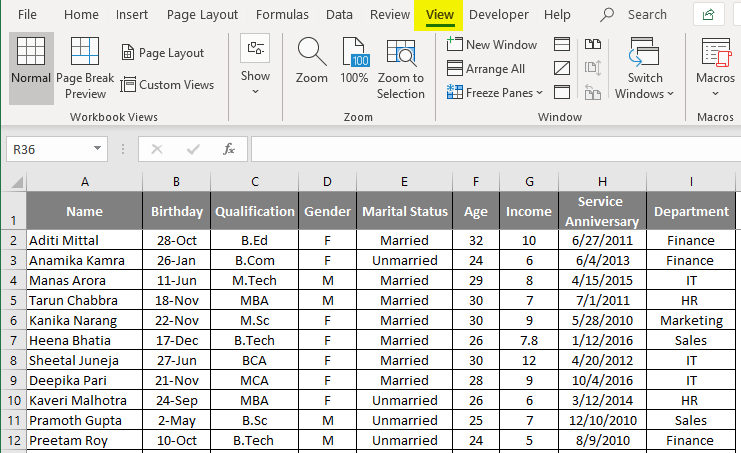
2. Go to the View tab. This is located at the very top, inbetween «Review» and «Add-ins.»
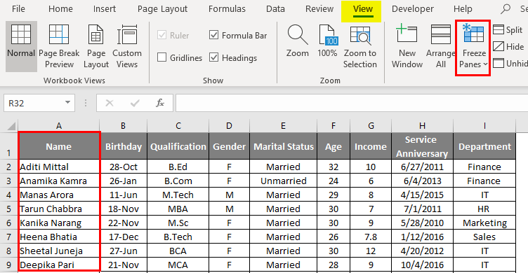
3. Select the Freeze Panes option and click «Freeze Panes.» This selection can be found in the same place where «New Window» and «Arrange All» are located.
That’s all there is to it. As you can see in our example, the frozen rows will stay visible when you scroll down. You can tell where the rows were frozen by the green line dividing the frozen rows and the rows below them.
If you want to unfreeze the rows, go back to the Freeze Panes command and choose «Unfreeze Panes».
Note that under the Freeze Panes command, you can also choose «Freeze Top Row,» which will freeze the top row that’s visible (and any others above it) or «Freeze First Column,» which will keep the leftmost column visible when you scroll horizontally.
Besides allowing you to compare different rows in a long spreadsheet, the freeze panes feature lets you keep important information, such as table headings, always in view.
Need more Excel tricks? Check out our tutorials on How to Lock Cells in Excel and How to Use VLOOKUP in Excel.
Get instant access to breaking news, the hottest reviews, great deals and helpful tips.
Содержание
- Freeze panes to lock rows and columns
- Freeze rows or columns
- Unfreeze rows or columns
- Need more help?
- Freeze Cells in Excel
- How to Freeze Cells in Excel? (with Examples)
- Example #1
- Example #2
- Use of Rows & Column Freezing in Excel Cell
- Things to Remember
- Recommended Articles
- Freeze Columns in Excel
- #1 Freeze the First Column in Excel
- Example #1
- #2 Freeze Multiple Columns in Excel
- Example #2
- #3 Freeze the Row and Column Together in Excel
- Example #3
- #4 Unfreeze Panes in Excel
- The Rules of Freezing in Excel
- Frequently Asked Questions
- Recommended Articles
Freeze panes to lock rows and columns
To keep an area of a worksheet visible while you scroll to another area of the worksheet, go to the View tab, where you can Freeze Panes to lock specific rows and columns in place, or you can Split panes to create separate windows of the same worksheet.
Freeze rows or columns
Freeze the first column
Select View > Freeze Panes > Freeze First Column.
The faint line that appears between Column A and B shows that the first column is frozen.
Freeze the first two columns
Select the third column.
Select View > Freeze Panes > Freeze Panes.
Freeze columns and rows
Select the cell below the rows and to the right of the columns you want to keep visible when you scroll.
Select View > Freeze Panes > Freeze Panes.
Unfreeze rows or columns
On the View tab > Window > Unfreeze Panes.

Note: If you don’t see the View tab, it’s likely that you are using Excel Starter. Not all features are supported in Excel Starter.
Need more help?
You can always ask an expert in the Excel Tech Community or get support in the Answers community.
Источник
Freeze Cells in Excel


How to Freeze Cells in Excel? (with Examples)
Freezing cells in Excel means that when we move down to the data or move up the cells, it freezes the cells displayed on the window. To freeze cells in Excel, we must select those cells we want to freeze. Then, in the “View” tab in the windows section, click on “Freeze Panes” and again click on “Freeze Panes” from the drop-down list. As a result, this will freeze the selected cells. First, let us understand how to freeze rows and columns in Excel by a simple example.
Table of contents
Example #1
Freezing the Rows: Given below is a simple example of a calendar.
- We must first select the row which we need to freeze the cell by clicking on the number of the row.

Then, click on the “View” tab on the ribbon. Next, we must select the “Freeze Panes” command on the “View” tab.
The selected rows get frozen in their position, and a grey line denotes it. We can scroll down the entire worksheet and continue viewing the frozen rows at the top. As we can see in the snapshot below, the rows above the grey line are frozen and do not move after we scroll the worksheet.
We can repeat the same process for unfreezing the cells. Once we have frozen the cells, the same command is changed in the “View” tab. The “Freeze Panes” in the Excel command is now changed to the “Unfreeze Panes” command. By clicking on it, the frozen cells are unfrozen. This command unlocks all the rows and columns to scroll through the worksheet.

The date is provided in the columns instead of the rows in this example.
For unfreezing the columns, we must use the same process as we did in the case of rows by using the “Unfreeze Panes” command from the “View” tab. In addition, there are two other commands in the “Freeze Panes” options: “Freeze Top Row” and “Freeze First Column.”

These commands are used only for freezing the top row and the first column, respectively. For example, the “Freeze Top Row” command freezes the row number “1,” and the “Freeze First Column” command freezes the column number A cell. It is to be noted that we can also freeze rows and columns together. In addition, It is not necessary to lock only the row or the column at a single instance.
Example #2
Let us take an example of the same.
- Step 1: The sheet below shows the timesheet of a company. The columns contain the headers as “Day,” “Date,” “Regular Hours,” “Overtime Hours,” “Sick,” “Vacation,” and “Total.”
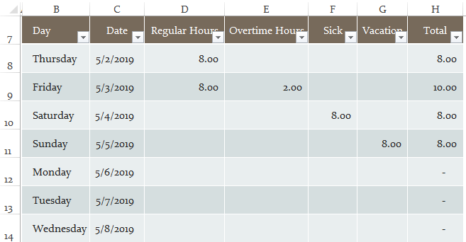
- Step 2: We need to see columns “B” and row 7 throughout the worksheet. We have to select the cell above, besides which we need to freeze the columns and rows cells, respectively. In our example, we have to choose the cell number H4.

- Step 3: After selecting the cell, we need to click on the “View” tab on the ribbon and select the “Freeze Panes” command on the “View” tab.
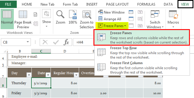
- Step 4: As we can see from the snapshot below, two grey lines denote the locking of cells.
Use of Rows & Column Freezing in Excel Cell
If we use the “Freeze Panes” command to freeze the columns and rows of Excel cells, they will remain displayed on the screen regardless of the magnification settings that we select or how we scroll through the cells. Let us take a practical example of the weekly attendance report of a class.
- Step 1: Now, if we take a look at the snapshot below, the rows and columns display various pieces of information such as “Student name,” “Name of the days,” “Room,” etc. The topmost column shows the “logo to be placed here” and the “Weekly Attendance Report.”

In this case, it becomes necessary to freeze certain Excel columns and rows of cells to understand the attendance of the reports. Otherwise, the report becomes vague and difficult to understand.
- Step 2: We must select the cell at the F4 location as we need to freeze down the rows up to the subject code P1, T1, U1, E1, and columns up to the “Student Name.”
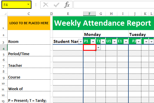
- Step 3: Once we select the cell, we must use the “Freeze Panes” command, freezing the cells at the position indicating a grey line.
As a result, we can see that the rows and columns beside and above the selected cell have been frozen, as shown in the snapshots below.
Similarly, we can use the “Unfreeze Panes” command from the “View” tab to unlock the cells which we have frozen.
Hence, explaining the examples above, we used the freezing of rows and columns in Excel.
Things to Remember
- When we press the “Ctrl+Home” Excel Shortcut keysExcel Shortcut KeysAn Excel shortcut is a technique of performing a manual task in a quicker way.read more after giving the “Frozen Panes” command in a worksheet, instead of positioning the cell cursor in cell A1 as normal, Excel sets the cell cursor in the first unfrozen cell.
- The “Freeze Panes” in the worksheet cell display consist of a feature for printing a spreadsheet known as “Print Titles.” When we use Print TitlesPrint TitlesIn Excel, Print Titles is a feature that lets the users print specific row & column headings on every page of a multi-page report. You need to select “Print Titles” in the Page Layout Tab & enter the required details to perform the function.read more in a report, the columns and rows that we define as the titles are printed at the top and to the left of all data on each report page.
- The shortcut keys that get random access to the “Freezing Panes” command are “Alt+W+F.”
- In the case of freezing Excel rows and columns together, we must select the cell above, and the rows and columns need to be frozen. We do not have to select the entire row and column together for locking.
Recommended Articles
This article is a guide to Freeze Cells in Excel. We discuss how to freeze rows and columns using the “Freeze Panes” command in Excel with some examples and a downloadable Excel template. You may learn more about Excel from the following articles: –
Источник
Freeze Columns in Excel
Freezing columns in excel fixes or locks them so that they remain visible while scrolling through the database. A frozen column does not move with the movement of the remaining columns.
For example, freezing the first column (column A) ensures that it stays at its place at the time of navigation through the rest of the columns. Moreover, if column A consists of headings, the user may want to view these while working on the other columns of the dataset.
The objectives of freezing an excel column are:
- To ensure that the user does not lose track of the specific column
- To facilitate comparison of different columns of the worksheet
Freezing columns prevents the user from referring to the same column again and again. In other words, the frozen columns save the scrolling time of the user.
All the properties of the frozen column apply to the frozen row as well.
- Freeze panes–It freezes multiple rows and columns.
- Freeze top row–It freezes only the first row.
- Freeze first column–It freezes only the first column.
After freezing a row or column in excel, a grey line appears at the end of the frozen area. This line indicates that the row or column has been frozen.
Table of contents
Let us go through the ways of freezing the first excel column, multiple columns, and both rows and columns.
#1 Freeze the First Column in Excel
Freezing the first column locks column A of the worksheet. This means that on moving from left to right, this column will be visible at all times.
In addition, column A is fixed irrespective of the column from which the actual data begins. The excel shortcut to freeze the first column is “Alt+W+F+C” (when pressed one by one).
Let us consider an example.
Example #1
The following table shows the sales revenue (in $) generated by the products of specific segments. The data relates to various countries and is spread across the first five months of the year 2015.
We want to freeze the first excel column (column A).
In order to view the column “segment” on a movement from left to right, we need to freeze it.
The steps for freezing the excel column are listed as follows:
- Select the worksheet where the first column is to be frozen.
In the View tab, click the “freeze panes” drop-down under the “window” section. Select “freeze first column,” as shown in the succeeding image.
Alternatively, press the shortcut keys “Alt+W+F+C” one by one.
The first column is frozen. The grey line appears at the end of column A indicating that the column to the left is frozen. The column AB shown in the following image is the last scrolled column of the dataset.
On scrolling (from left to right) through the remaining columns of the dataset, column A is visible. The same is shown in the following image.
In the same way, the first row can be frozen.
#2 Freeze Multiple Columns in Excel
Freezing multiple excel columns is similar to freezing multiple rows. For freezing multiple columns, select the first right-hand side cell immediately after the last column to be frozen. This is because multiple columns are frozen based on the current selection.
Similarly, for freezing multiple rows, select the first cell immediately below the last row to be frozen.
For example, to freeze the columns A, B, and C, select the cell D1. By freezing the first three columns, they remain visible to the user at all times. Likewise, to freeze the rows 1, 2, and 3, select the cell A4.
The shortcut to freeze multiple excel columns is “Alt+W+F+F” (when pressed one by one).
Let us consider an example.
Example #2
Working on the data of example #1, we want to freeze the first four columns, A, B, C, and D.
The steps for freezing multiple excel columns are listed as follows:
Step 1: Select the cell E1. This is because the first four columns are to be frozen.
Step 2: In the View tab, click the “freeze panes” drop-down under the “window” section. Select “freeze panes,” as shown in the succeeding image.
Alternatively, press the shortcut keys “Alt+W+F+F” one by one.
Step 3: The first four columns are frozen. The grey line appears (shown in the following image) at the end of column D, indicating that the columns to the left are frozen.
The columns R and S shown in the following image are the scrolled columns towards the end of the dataset.
Step 4: On scrolling (from left to right) till the last column of the dataset, the first four columns are visible. The same is shown in the following image.
#3 Freeze the Row and Column Together in Excel
Usually, the first row and the first column of a database contain headers. The user might want to view the row 1 and the column A simultaneously and at all times. Hence, it is essential to lock them together to permit their visibility while scrolling down and from left to right.
The only difference between the methods #2 and #3 is in the selection of the cell (step 1). With the “freeze panes” option, Excel freezes the rows and columns preceding the current active cell.
The shortcut to freeze the row and column together is “Alt+W+F+F” (when pressed one by one).
Let us consider an example.
Example #3
Working on the data of example #1, we want to freeze the first row (row 1) and the first column (column A) at the same time.
The steps to freeze the excel row 1 and column A together are listed as follows:
Step 1: Select the cell B2.
Step 2: Press the shortcut keys “Alt+W+F+F” one by one. It freezes the column to the left of the selected cell B2. At the same time, the row preceding the active cell (B2) is also frozen, as shown in the following image.
Hence two grey lines appear, one at the end of row 1 (horizontal) and the other at the end of column A (vertical).
Note: Alternatively, the “freeze panes” option can be selected from the “freeze panes” drop-down of the View tab.
Step 3: On scrolling from top to bottom and left to right, the row 1 and column A are visible. The same is shown in the following image.
Note: It is possible to freeze as many rows and columns depending on the requirement. The condition is that freezing of multiple excel rows and columns should begin with the top row (row 1) and the first column (column A).
#4 Unfreeze Panes in Excel
Unfreezing of panes does not require any cells to be selected. The steps to unfreeze panes in Excel are listed as follows:
Step 1: In the View tab, click the “freeze panes” drop-down under the “window” section. Select “unfreeze panes,” as shown in the succeeding image.
Alternatively, press the shortcut keys “Alt+W+F+F” one by one.
Step 2: The grey lines are removed, as shown in the following image.
Note: The “unfreeze panes” option appears only after freezes have been applied to the Excel worksheet.
The Rules of Freezing in Excel
The norms governing the freezing of rows and columns are listed as follows:
- It is not possible to freeze excel rows and columns in the middle of the worksheet.
- The option “freeze panes” can be applied only once. It is not possible to create multiple “freeze panes” in a single worksheet.
- The rows and columns to be fixed should be visible at the time of freezing. Otherwise, they will remain hidden even after freezing.
Note 1: To divide a worksheet into two or more areas with separate scroll bars Scroll Bars In Excel, there are two scroll bars: one is a vertical scroll bar that is used to view data from up and down, and the other is a horizontal scroll bar that is used to view data from left to right. read more for each, use the “split” option. This is available in the “window” section of the View tab.
Note 2: To fix the header row of a large dataset that does not fit into the screen, create an Excel table Excel Table In excel, tables are a range with data in rows and columns, and they expand when new data is inserted in the range in any new row or column in the table. To use a table, click on the table and select the data range. read more . Moreover, ensure the visibility of this row by selecting any cell within the table before scrolling.
Frequently Asked Questions
Freezing a column means locking it in order to keep it visible while the user scrolls through the database. This is specifically helpful if a column contains headers which are required to be seen at all times.
After freezing, a grey line appears to indicate the frozen columns on its left. The steps to freeze the first column (column A) are listed as follows:
• In the View tab, click the “freeze panes” drop-down under the “window” section.
• Select “freeze first column.” Alternatively, press the shortcut keys “Alt+W+F+C” one by one.
• The first column (column A) is frozen.
Note: For freezing the first row, select “freeze top row” from the “freeze panes” drop-down of the View tab.
Let us freeze columns A, B, C, D, and E. The steps to freeze multiple columns in Excel are listed as follows:
• Select either the column or the first cell to the right of the last column to be frozen (column E). So, select either column F or the cell F1.
• In the View tab, click the “freeze panes” drop-down under the “window” section.
• Select “freeze panes.” Alternatively, press the shortcut keys “Alt+W+F+F” one by one.
• The columns A B, C, D, and E are frozen as indicated by the grey line at the end of column E.
Let us freeze rows 1, 2, and 3 and columns A, B, and C. The steps to freeze the given rows and columns together are listed as follows:
• Select cell D4 based on the following parameters:
a. It immediately follows the last row to be frozen (row 3).
b. It is to the right of the last column to be frozen (column C).
• In the View tab, click the “freeze panes” drop-down under the “window” section.
• Select “freeze panes.” Alternatively, press the shortcut keys “Alt+W+F+F” one by one.
• The rows 1, 2, and 3 and columns A, B, and C are frozen. This is indicated by the grey line appearing below row 3 and at the end of column C.
Note: The freezing of multiple excel rows and columns should begin with the top row (row 1) and the first column (column A).
Recommended Articles
This has been a guide to freezing columns in Excel. Here we discuss how to freeze the first column, multiple columns, and both rows and columns. For more on Excel, take a look at the following articles-
Источник
Suppose we create a large table in excel spreadsheet and it lists large amount of data. There are headers in the first row, and if we want to drag the scroll bar to view the bottom of table, the headers are hidden due to it lists on the top. So, in this case if we want to see the headers all the time, we need to freeze the first row to make it fixed and always displays on the top even we drag the scrollbar. On the other side, sometimes we need to freeze more rows, or columns, or even freeze row and column simultaneously. To implement this, we need to know the way to freeze row and columns. This article will introduce different ways to freeze row and columns with examples for you, you can’t miss it.
Table of Contents
- Method 1: How to Freeze the First Row in Excel Spreadsheet
- Method 2: How to Freeze Multiple Rows in Excel Spreadsheet
- Method 3: How to Freeze the First Column in Excel Spreadsheet
- Method 4: How to Freeze Row and Column in Excel Spreadsheet
- Method 5: How to Freeze Rows and Columns in Excel Spreadsheet
Method 1: How to Freeze the First Row in Excel Spreadsheet
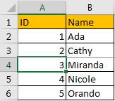
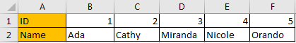
In most daily work, freeze the first row in table is frequently needed due to in most tables the first row lists the headers. So, people always want to see the headers on top no matter whether they drag the scrollbar to the end or not. See example below:
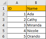
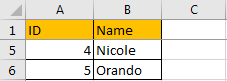
Suppose it lists a long list of ID and names. Header ID and Name are listed on the top. Now let’s freeze the first row.
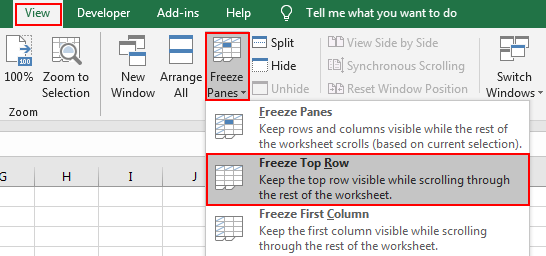
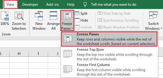
Step 1: Click View in the ribbon, then click Freeze Panes in Window group, then click the small triangle of Freeze Panes to load below three options, select the middle one ‘Freeze Top Row’.
Step 2: After above operating. The first top row is fixed and always displayed on the top. Try to drag the scrollbar. You can see the header row is stayed on the top.
Method 2: How to Freeze Multiple Rows in Excel Spreadsheet
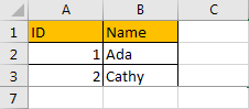
If you want to freeze the first three rows in excel, you can just select the first cell in the fourth row, then freeze the rows above the selected cell. See details below.
Step 1: Click A4 in the table.
Step 2: Click View in the ribbon, then click Freeze Panes in Window group, then click the small triangle of Freeze Panes to load below three options, select the first one ‘Freeze Panes’.
Step 3: Try to drag the scrollbar. Verify that top three rows are fixed.
Method 3: How to Freeze the First Column in Excel Spreadsheet
See screenshot below:
Now let’s freeze the first column. The way is similar with freeze the first row.
Step 1: Click View in the ribbon, then click Freeze Panes in Window group, then click the small triangle of Freeze Panes to load below three options, select the middle one ‘Freeze First Column’.
Step 2: Verify if it works well.
Obviously, it works.
Method 4: How to Freeze Row and Column in Excel Spreadsheet
If you want to just freeze the first row and column, just click on B2. Then click View->Freeze Panes->Freeze Panes in Window group.

Method 5: How to Freeze Rows and Columns in Excel Spreadsheet
If you want to freeze multiple rows and columns, refer to the description of Freeze Panes ‘Keep rows and column visible while the rest of the worksheet scrolls (based on current selection)’ we can know that we can select a cell to make it as the first cell outside of your fixed area. For example, if we want to freeze the top three rows and first two columns (row 4 is not fixed and column C is not fixed), we can click on C4, then repeat above steps to freeze panes.
I recently helped a friend with Excel, and when I asked him how the spreadsheet looked, he hesitated. Finally, he looked at me and said, “It’s overwhelming.” The data was OK, but he wanted to see the top row when he scrolled. The solution was to show him how to freeze rows and columns in Excel so that key headings or cells were always visible. I’ve outlined four scenarios and solution steps.
This was a good communication lesson for me. It reminded me that we all have different skill levels and vocabularies. For example, when you’re new, you’re probably not thinking in terms like “how to freeze panes in Excel.” You may not know what a pane is. It’s not describing your problem. My friend was thinking in terms of a “sticky header,” or “Excel floating header,” or “pinning rows.” I wasn’t thinking of any of those.
Let’s Start with Excel Panes
An Excel pane is a set of columns and rows defined by cells. You get to determine the size, shape, and location. For many people, it might be the top row. For others, it’s an inverted L-shape and contains the top row and first column. You’re the spreadsheet architect and can define your pane.
Regarding spreadsheets, you can “freeze panes” or “split panes.” Splitting panes is a bit more complex because you have separate windows of your data on the worksheet. So, for the sake of simplicity, this tutorial will cover freezing panes.
If your columns and rows aren’t in the orientation you want, you may want to learn how to transpose or switch columns and rows in Excel.
Why Lock Spreadsheet Cells?
A key benefit to locking or freezing cells is seeing the important information regardless of scrolling. The split pane data stays fixed. Your spreadsheet can contain panes with column headings, multiple rows, multiple columns, or both.
Otherwise, losing focus on a large worksheet is easy when you don’t have column headings or identifiers. I’ve had times where I’ve entered data only to see I was one cell off and produced Excel formula errors. By locking various sections, you have a consistent reference point. This also helps readability.
Typically, the cells you want to stay sticky are labels like headers. However, they could just as easily be an entire column, such as employee names.
Let’s go through four examples and keyboard shortcuts to freeze panes in Excel.
1 – How to Freeze the Top Row
This freeze row example is perhaps the most common because people like to lock the top row that contains headers, such as in the example below.
Another solution is to format the spreadsheet as an Excel table.
- Open your worksheet.
- Click the View tab on the ribbon.
- On the Freeze Panes button, click the small triangle ▼ (drop-down arrow) in the lower right corner. You should see a new menu with three options.

- Click the menu option Freeze Top Row.
- Scroll down your sheet to ensure the first row stays locked at the top.
You should see a darker border under row 1.
Keyboard Shortcut – Lock Top Row
I like to do this shortcut slowly the first time to see the ALT key letter assignments as you type. I can see the keyboard assignments in the example below once I hit my Alt key. Some people prefer to add the Freeze Panes command to the Quick Access toolbar because they frequently use it.

Alt + w + f + r
2 – How to Freeze the First Column
A similar scenario is when you want to freeze the leftmost column. I guess Microsoft researched this to determine the most common sub-menu options.
I find this option helpful when I have a spreadsheet with many columns and I need to fill in data without using an Excel data form.

- Open your Excel worksheet.
- Click the View tab on the ribbon.
- On the Freeze Panes button, click the small triangle ▼. You should see a new menu with your 3 options.
- Click the option Freeze First Column.
- Scroll across your sheet to make sure the left column stays fixed.
Keyboard Shortcut – Lock First Column
Alt + w + f + c
3 – How to Freeze the Top Row & First Column
This is my favorite option. If you look at Microsoft’s initial Freeze Panes options, there isn’t one for the top row and first column. Instead, we’ll use the generic option called Freeze Panes.
The subtext reads, “Keep rows and columns visible while the rest of the worksheet scrolls (based on current selection).” Some folks get confused as they think they have to highlight data to make a selection.
Instead, consider the selection of the first cell outside your fixed column and row. If I wanted to lock the top row and top column, that selection cell would be cell B2 or Nevada. Regardless of whether I scroll down or to the right, the first cell that disappears when I scroll is B2.

- Open your Excel spreadsheet.
- Click cell B2. (Your set cell.)
- Click the View tab on the ribbon.
- On the Freeze Panes button, click the small triangle ▼ in the lower right corner. You should see a dropdown menu with your 3 options.
- Click the option Freeze Panes.
- Scroll down your worksheet to make sure the first row stays at the top.
- Scroll across your sheet to make sure your first column stays locked on the left.
Keyboard Shortcut – Freeze Panes
Alt + w + f + f
4 – Freeze Multiple Columns or Rows
On occasion, I get some Excel worksheets where the author puts descriptive text above the data. My header isn’t in Row 1 but further down in Row 5. Or I want to lock multiple columns to the left. In the example below, I want to lock Columns A & B and Rows 1-5.

The process is the same, I just need to click the set cell that stops the fixed area. In this case, it would be cell C6 or “Regions Field.” The content above and to the left is frozen.
Everything in the red boxes would be locked. The downside is you may give up much of the screen real estate.
Why Freeze Panes May Not Work
There are some rules surrounding this feature. If you don’t follow these, freeze panes may not work.
Quick test: If you type Ctrl + Home and your cursor moves to cell A1, you haven’t locked anything.
- If you dislike your settings, use the Unfreeze Panes command.
- This feature won’t work on a protected worksheet or Page Layout View.
- If you’re editing a value in the Formula bar, the View menu will be disabled.
If you need to see the same header on printed pages, Microsoft has instructions.
As you’ve seen, choosing what content to freeze is easy. You can freeze the top row, first column, both, or a subset of your data, depending on what you want to do with it. The flexibility is part of what makes Microsoft Excel such an excellent program for organizing and analyzing information from any field.
Excel Freeze Columns (Table of Contents)
- What are Freeze Columns in Excel?
- How to Freeze Columns in Excel?
What are Freeze Columns in Excel?
Freeze helps us fix the select Column so that we can see the data towards the most right in the worksheet. Freeze Column can be accessed from the View menu tab’s Window section from the drop-down list of Freeze Panes. First, to freeze the column, select the column which we want to freeze or put the cursor anywhere in that column and then select the Freeze Column option from the list. We will be able to see the selected column is now frozen.
Why Freeze Panes?
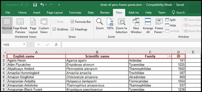
When you are working on data that are large, you may not be able to view some of the data because it does not fit on the screen. So let’s take a look at the below excel sheet. As you can see in the above screenshot, you can only see column U and Row 23. So if you have headers in Row 1 and you scroll down or right, the headers will not be visible.
This is where Freeze Panes come for help. Freeze panes can keep rows or columns visible while scrolling the rest of the worksheet.
How to Freeze Columns in Excel?
Freeze Panes come with three options, and we will take a look at all of them one by one with examples.
You can download this Freeze Columns Excel Template here – Freeze Columns Excel Template
Example #1 – Freeze Top Row
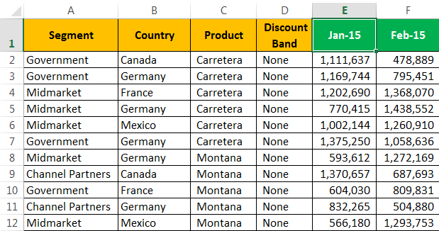
As you can see in the below Excel screenshot, Row 1 is the header for my report, which contains Employee’s personal information, and I want the headers to be visible all the time.
But when I scroll down now, I will not be able to see the header row.
So to keep the first row visible, I need to Freeze Top row. To Freeze the top row, we need to execute the following steps:
- Select Row 1 as shown in the below screenshot.
- Go to the View Tab in the Excel Sheet.
- Select Freeze Panes.
- In the drop-down list, select Freeze Top Row.
- So after selecting Freeze Top Row, you will be able to freeze row 1, and you can scroll all the data below Row 1 without losing visibility to the headers.
Example #2 – Freeze First column
Now, if you have important information in Column A which you want to be visible when you scroll towards the right, you need to use the Freeze the First Column option.
Suppose, in our first example; I want to freeze the Employee Names in Column A. You will need to follow the below steps.
- Select Column A
- Go to the View Tab in the Excel Sheet.
- Select Freeze Panes.
In the drop-down list, select Freeze First Column.
Now when you scroll towards the right, you can scroll without losing the visibility to column A.
Example #3 – Freeze Panes
To Freeze any pane in the sheet, either it’s a row or column, you need to select the Freeze Panes option from the drop-down list. This option is not for Top Row and First Column; it will freeze your screen from any row or column which you want to freeze and scroll the rest of the data.
You need to follow the below steps to use this option. Go to the View Tab in Excel Sheet and Select Freeze Panes.
- Before selecting the freeze pane, you need to select the cell from where you want to freeze the pane.
- In the below example, if I need to freeze data till Qualification and I want to freeze the top row, I will select cell D2 and click Freeze Panes.
Now, as you can see, data till column C and row 1 is always visible even if you scroll down or scroll towards the right.
How to Unfreeze the Freeze Panes?
If you want to unfreeze the pane and come back to the earlier view, you just need to follow the below steps.
- Select the Row or Column, which is already Freeze.
- Go to the View Tab in Excel Sheet and Select Freeze Panes; in the Drop-Down list, select Unfreeze pane so the row or column will be Unfreeze as shown in the below screenshot.
Things to Remember About Freeze Columns in Excel
- If the Worksheet is in Protected mode, then you cannot Freeze or Unfreeze Panes.
- It is very important that while printing anything, you need to Unfreeze panes as the Rows or Columns which are frozen will not come while Printing the Worksheet.
- If you are in cell editing mode or page layout view, you will not be able to Freeze or Unfreeze Panes.
Recommended Articles
This is a guide to Freeze Columns in Excel. Here we discuss how to freeze columns in excel along with practical examples and a downloadable excel template. You can also go through our other suggested articles –
- Excel Freeze Rows
- Excel Freeze Panes
- Column Header in Excel
- COLUMNS Formula in Excel