
![]()
Download Article
![]()
Download Article
- Freezing the First Column or Row
- Freezing Multiple Columns or Rows
- Video
- Q&A
|
|
|
This wikiHow teaches you how to freeze specific rows and columns in your Microsoft Excel worksheet. Freezing rows or columns ensures that certain cells remain visible as you scroll through the data. If you want to easily edit two parts of the spreadsheet at once, splitting your panes will make the task much easier.
-

1
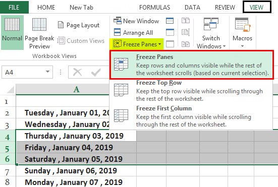
Click the View tab. It’s at the top of Excel. Frozen cells are rows or columns that remain visible while you scroll through a worksheet.[1]
If you want column headers or row labels to remain visible as you work with large amounts of data, you’ll likely find it helpful to lock those cells into place.- Only whole rows or columns can be frozen. It is not possible to freeze individual cells.
-
2
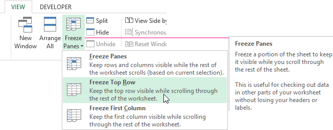
Click the Freeze Panes button. It’s in the «Window» section of the toolbar. A set of three freezing options will appear.
Advertisement
-
3
Click Freeze Top Row or Freeze First Column. If you want to keep the top row of cells in place as you scroll down through your data, select Freeze Top Row. To keep the first column in place as you scroll horizontally, select Freeze First Column.
-
4
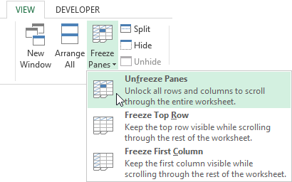
Unfreeze your cells. If you want to unlock the frozen cells, click the Freeze Panes menu again and select Unfreeze Panes.


Advertisement
-
1
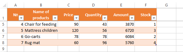
Select the row or column after those you want to freeze. If the data you want to keep stationary takes up more than one row or column, click the column letter or row number after those you want to freeze. For example:
- If you want to keep rows 1, 2, and 3 in place as you scroll down through your data, click row 4 to select it.
- If you want columns A and B to remain still as you scroll sideways through your data, click column C to select it.
- Frozen cells must connect to the top or left edge of the spreadsheet. It’s not possible to freeze rows or columns in the middle of the sheet.[2]
-
2
Click the View tab. It’s at the top of Excel.
-
3
Click the Freeze Panes button. It’s in the «Window» section of the toolbar. A set of three freezing options will appear.
-
4
Click Freeze Panes on the menu. It’s at the top of the menu. This freezes the columns or rows before the one you selected.
-
5
Unfreeze your cells. If you want to unlock the frozen cells, click the Freeze Panes menu again and select Unfreeze Panes.


Advertisement
Add New Question
-
Question
How do I freeze the top two rows?

Select the row directly under the rows you want to freeze (in this case, the third row). Go to View, Freeze Panes, and select «Freeze Panes.» Everything above the row you have selected will be frozen.
Ask a Question
200 characters left
Include your email address to get a message when this question is answered.
Submit
Advertisement
Thanks for submitting a tip for review!
wikiHow Video: How to Freeze Cells in Excel
About This Article
Article SummaryX
1. Click View.
2. Click Freeze Panes.
3. Select Freeze Top Row or Freeze First Column.
Did this summary help you?
Thanks to all authors for creating a page that has been read 171,421 times.
Is this article up to date?
Freeze panes to lock rows and columns
To keep an area of a worksheet visible while you scroll to another area of the worksheet, go to the View tab, where you can Freeze Panes to lock specific rows and columns in place, or you can Split panes to create separate windows of the same worksheet.

Freeze rows or columns
Freeze the first column
-
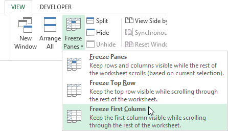
Select View > Freeze Panes > Freeze First Column.
The faint line that appears between Column A and B shows that the first column is frozen.
Freeze the first two columns
-
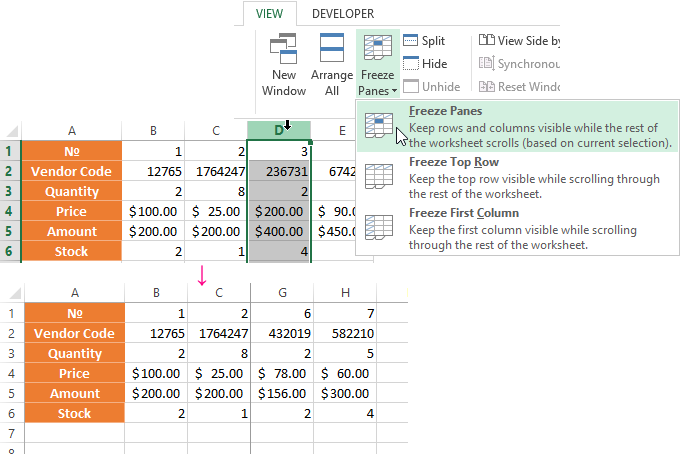
Select the third column.
-
Select View > Freeze Panes > Freeze Panes.
Freeze columns and rows
-
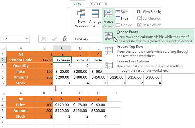
Select the cell below the rows and to the right of the columns you want to keep visible when you scroll.
-
Select View > Freeze Panes > Freeze Panes.
Unfreeze rows or columns
-
On the View tab > Window > Unfreeze Panes.
Note: If you don’t see the View tab, it’s likely that you are using Excel Starter. Not all features are supported in Excel Starter.
Need more help?
You can always ask an expert in the Excel Tech Community or get support in the Answers community.
See Also
Freeze panes to lock the first row or column in Excel 2016 for Mac
Split panes to lock rows or columns in separate worksheet areas
Overview of formulas in Excel
How to avoid broken formulas
Find and correct errors in formulas
Keyboard shortcuts in Excel
Excel functions (alphabetical)
Excel functions (by category)
Need more help?
Want more options?
Explore subscription benefits, browse training courses, learn how to secure your device, and more.
Communities help you ask and answer questions, give feedback, and hear from experts with rich knowledge.
How to Freeze Cells in Excel? (with Examples)
Freezing cells in Excel means that when we move down to the data or move up the cells, it freezes the cells displayed on the window. To freeze cells in Excel, we must select those cells we want to freeze. Then, in the “View” tab in the windows section, click on “Freeze Panes” and again click on “Freeze Panes” from the drop-down list. As a result, this will freeze the selected cells. First, let us understand how to freeze rows and columns in Excel by a simple example.
You can download this Freeze Rows and Columns Excel Cell template here – Freeze Rows and Columns Excel Cell template
Table of contents
- How to Freeze Cells in Excel? (with Examples)
- Example #1
- Example #2
- Use of Rows & Column Freezing in Excel Cell
- Things to Remember
- Recommended Articles
Example #1
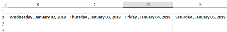
Freezing the Rows: Given below is a simple example of a calendar.
- We must first select the row which we need to freeze the cell by clicking on the number of the row.

- Then, click on the “View” tab on the ribbon. Next, we must select the “Freeze Panes” command on the “View” tab.

- The selected rows get frozen in their position, and a grey line denotes it. We can scroll down the entire worksheet and continue viewing the frozen rows at the top. As we can see in the snapshot below, the rows above the grey line are frozen and do not move after we scroll the worksheet.

- We can repeat the same process for unfreezing the cells. Once we have frozen the cells, the same command is changed in the “View” tab. The “Freeze Panes” in the Excel command is now changed to the “Unfreeze Panes” command. By clicking on it, the frozen cells are unfrozen. This command unlocks all the rows and columns to scroll through the worksheet.

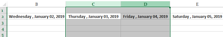
The date is provided in the columns instead of the rows in this example.
- Step 1: We need to select the columns, which we need to freeze Excel cells by clicking on the alphabet of the column.
- Step 2: After selecting the columns, we need to click on the “View” tab on the ribbon. Then, we need to choose the “Freeze Panes” command on the “View” tab.

- Step 3: The selected columns get frozen in their position, and a grey line denotes it. We can scroll the entire worksheet and continue viewing the frozen columns. As we can see in the snapshot below, the columns beside the grey line are frozen and do not move after we scroll the worksheet.
For unfreezing the columns, we must use the same process as we did in the case of rows by using the “Unfreeze Panes” command from the “View” tab. In addition, there are two other commands in the “Freeze Panes” options: “Freeze Top Row” and “Freeze First Column.”

These commands are used only for freezing the top row and the first column, respectively. For example, the “Freeze Top Row” command freezes the row number “1,” and the “Freeze First Column” command freezes the column number A cell. It is to be noted that we can also freeze rows and columns together. In addition, It is not necessary to lock only the row or the column at a single instance.
Example #2
Let us take an example of the same.
- Step 1: The sheet below shows the timesheet of a company. The columns contain the headers as “Day,” “Date,” “Regular Hours,” “Overtime Hours,” “Sick,” “Vacation,” and “Total.”
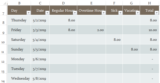
- Step 2: We need to see columns “B” and row 7 throughout the worksheet. We have to select the cell above, besides which we need to freeze the columns and rows cells, respectively. In our example, we have to choose the cell number H4.

- Step 3: After selecting the cell, we need to click on the “View” tab on the ribbon and select the “Freeze Panes” command on the “View” tab.
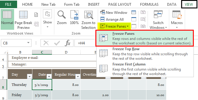
- Step 4: As we can see from the snapshot below, two grey lines denote the locking of cells.
Use of Rows & Column Freezing in Excel Cell
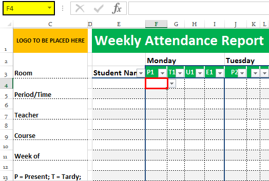
If we use the “Freeze Panes” command to freeze the columns and rows of Excel cells, they will remain displayed on the screen regardless of the magnification settings that we select or how we scroll through the cells. Let us take a practical example of the weekly attendance report of a class.
- Step 1: Now, if we take a look at the snapshot below, the rows and columns display various pieces of information such as “Student name,” “Name of the days,” “Room,” etc. The topmost column shows the “logo to be placed here” and the “Weekly Attendance Report.”

In this case, it becomes necessary to freeze certain Excel columns and rows of cells to understand the attendance of the reports. Otherwise, the report becomes vague and difficult to understand.
- Step 2: We must select the cell at the F4 location as we need to freeze down the rows up to the subject code P1, T1, U1, E1, and columns up to the “Student Name.”
- Step 3: Once we select the cell, we must use the “Freeze Panes” command, freezing the cells at the position indicating a grey line.
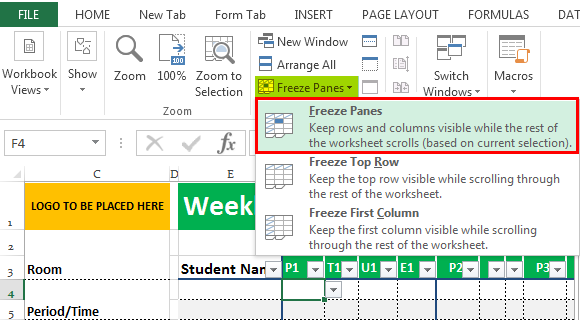
As a result, we can see that the rows and columns beside and above the selected cell have been frozen, as shown in the snapshots below.
Similarly, we can use the “Unfreeze Panes” command from the “View” tab to unlock the cells which we have frozen.
Hence, explaining the examples above, we used the freezing of rows and columns in Excel.
Things to Remember
- When we press the “Ctrl+Home” Excel Shortcut keysAn Excel shortcut is a technique of performing a manual task in a quicker way.read more after giving the “Frozen Panes” command in a worksheet, instead of positioning the cell cursor in cell A1 as normal, Excel sets the cell cursor in the first unfrozen cell.
- The “Freeze Panes” in the worksheet cell display consist of a feature for printing a spreadsheet known as “Print Titles.” When we use Print TitlesIn Excel, Print Titles is a feature that lets the users print specific row & column headings on every page of a multi-page report. You need to select “Print Titles” in the Page Layout Tab & enter the required details to perform the function. read more in a report, the columns and rows that we define as the titles are printed at the top and to the left of all data on each report page.
- The shortcut keys that get random access to the “Freezing Panes” command are “Alt+W+F.”
- In the case of freezing Excel rows and columns together, we must select the cell above, and the rows and columns need to be frozen. We do not have to select the entire row and column together for locking.
Recommended Articles
This article is a guide to Freeze Cells in Excel. We discuss how to freeze rows and columns using the “Freeze Panes” command in Excel with some examples and a downloadable Excel template. You may learn more about Excel from the following articles: –
- Freeze Columns in Excel
- How to Freeze Panes in Excel?
- What does Split Panes in Excel Mean?
- Hiding an Excel Column
Select the cell in the upper-left corner of the range you want to remain scrollable. Select View tab, Windows Group, click Freeze Panes from the menu bar. Excel inserts two lines to indicate where the frozen panes begin.
Contents
- 1 How do I freeze cells in Excel 2019?
- 2 What is the formula to freeze a cell in Excel?
- 3 Can you freeze 2 columns in Excel?
- 4 How do I freeze rows in Excel 2020?
- 5 What is F4 in Excel?
- 6 Why is F4 not working in Excel?
- 7 How do I lock cells in sheets?
- 8 How do I freeze 4 columns in Excel?
- 9 How do I freeze two columns in Excel 2021?
- 10 What is the shortcut key to freeze multiple columns in Excel?
- 11 How do you keep one cell constant in Excel?
- 12 How do you freeze columns A and B and rows 1 and 2?
- 13 How do I freeze 3 columns in Excel?
- 14 What does F11 do in Excel?
- 15 What does Alt R do in Excel?
- 16 What is Ctrl F3 in Excel?
- 17 What can I use instead of F4 in Excel?
- 18 How do I use F4 in Excel without FN?
- 19 How do I restrict editing in Excel?
- 20 How do I protect cells in Google Sheets 2021?
How do I freeze cells in Excel 2019?
Freezing Columns and Rows
- To freeze a set of columns and rows at the same time, click on the cell below and to the right of the panes you want to freeze.
- With the proper cell selected, select the “View” tab at the top and click on the “Freeze Panes” button, and select the “Freeze Panes” option in the drop-down.
What is the formula to freeze a cell in Excel?
Drag or copy formula and lock the cell value with the F4 key
For locking the cell reference of a single formula cell, the F4 key can help you easily. Select the formula cell, click on one of the cell reference in the Formula Bar, and press the F4 key. Then the selected cell reference is locked.
Can you freeze 2 columns in Excel?
To lock more than one row or column, or to lock both rows and columns at the same time, choose the View tab, and then click Freeze Panes.To lock multiple columns, select the column to the right of the last column you want frozen, choose the View tab, and then click Freeze Panes.
How do I freeze rows in Excel 2020?
How to freeze the top row in Excel
- Scroll your spreadsheet until the row you want to lock in place is the first row visible under the row of letters.
- In the menu, click “View.”
- In the ribbon, click “Freeze Panes” and then click “Freeze Top Row.”
- Select the row below the set of rows you want to freeze.
What is F4 in Excel?
When you are typing your formula, after you type a cell reference – press the F4 key. Excel automatically makes the cell reference absolute! By continuing to press F4, Excel will cycle through all of the absolute reference possibilities.
Why is F4 not working in Excel?
The problem isn’t in Excel, it’s in the computer BIOS settings. The function keys are not in function mode, but are in multimedia mode by default! You can change this so that you don’t have to press the combination of Fn+F4 each time you want to lock the cell.
How do I lock cells in sheets?
Lock Specific Cells In Google Sheets
- Right-click on the cell that you want to lock.
- Click on Protect range option.
- In the ‘Protected Sheets and ranges’ pane that opens up on the right, click on ‘Add a sheet or range’
- [Optional] Enter a description for the cell you’re locking.
How do I freeze 4 columns in Excel?
Freeze columns and rows
- Select the cell below the rows and to the right of the columns you want to keep visible when you scroll.
- Select View > Freeze Panes > Freeze Panes.
How do I freeze two columns in Excel 2021?
If you want to freeze multiple columns in Excel, you do that in the same way as you would freeze multiple rows.
- Select the column to the right of the column you want to freeze.
- Select the View tab and Freeze Panes.
- Select Freeze Panes.
What is the shortcut key to freeze multiple columns in Excel?
Here are the shortcuts for freezing rows/columns:
- To freeze the top row: ALT + W + F + R. Note that the top row gets fixed.
- To freeze the first column: ALT + W + F + C. Note that the left-most column gets fixed.
How do you keep one cell constant in Excel?
Keep formula cell reference constant with the F4 key
Select the cell with the formula you want to make it constant. 2. In the Formula Bar, put the cursor in the cell which you want to make it constant, then press the F4 key.
How do you freeze columns A and B and rows 1 and 2?
To freeze rows:
- Select the row below the row(s) you want to freeze. In our example, we want to freeze rows 1 and 2, so we’ll select row 3.
- Click the View tab on the Ribbon.
- Select the Freeze Panes command, then choose Freeze Panes from the drop-down menu.
- The rows will be frozen in place, as indicated by the gray line.
How do I freeze 3 columns in Excel?
How to freeze multiple columns in Excel
- Select the column to the right of the last column you want to freeze. For example, if you want to freeze the first 3 columns (A – C), select the entire column D or cell D1.
- And now, follow the already familiar path, i.e View tab > Freeze panes > and again Freeze panes.
What does F11 do in Excel?
F11 Creates a chart of the data in the current range in a separate Chart sheet. Shift+F11 inserts a new worksheet. Alt+F11 opens the Microsoft Visual Basic For Applications Editor, in which you can create a macro by using Visual Basic for Applications (VBA).
What does Alt R do in Excel?
In Microsoft Excel, pressing Alt + R opens the Review tab in the Ribbon. After using this shortcut, you can press an additional key to select a Review tab option.
What is Ctrl F3 in Excel?
You can bring up the Name Manager in Excel by pressing Ctrl + F3. This lists the names used in your current workbook, and you can also define new names, edit existing names or delete names from the Name Manager.
What can I use instead of F4 in Excel?
Laptop keyboards are smaller than stationary ones so typically, the F-keys (like F4) are used for something else. This is easily fixed! Just hold down the Fn key before you press F4 and it’ll work.
How do I use F4 in Excel without FN?
On Dell laptops you can hold the Fn key and press the Esc key that makes it work like a Caps lock and it toggles the function keys so that you can use F4 without pressing the Fn key but use the Fn key for the other function (eg.
How do I restrict editing in Excel?
To restrict editing to a sheet in Excel, use these steps:
- Open the Excel document.
- Click on File.
- Click on Info.
- On the right side, click the Protect Workbook menu.
- Select the Protect current sheet option.
- (Optional) Set a password to unlock the sheet.
- Check the Protect worksheet and contents of locked cells option.
How do I protect cells in Google Sheets 2021?
Click on “Data” > “Protected Sheets and Ranges.” Then choose between “Range” to protect a specific range of cells or “Sheet” to protect the entire spreadsheet.
Содержание
- Freeze panes to lock rows and columns
- Freeze rows or columns
- Unfreeze rows or columns
- Need more help?
- Freeze Cells in Excel
- How to Freeze Cells in Excel? (with Examples)
- Example #1
- Example #2
- Use of Rows & Column Freezing in Excel Cell
- Things to Remember
- Recommended Articles
- How to fix a row and column in Excel when scrolling
- Locking a row in Excel while scrolling
- Locking several rows in Excel while scrolling
- Freezing columns in Excel
- How to freeze the row and column in Excel
- Removing a fixed area in Excel
- How to freeze rows and columns in Excel
- How to freeze rows in Excel
- How to freeze top row in Excel
- How to freeze multiple rows in Excel
- How to freeze columns in Excel
- How to lock the first column
- How to freeze multiple columns in Excel
- How to freeze rows and columns in Excel
- How to unlock rows and columns in Excel
- Freeze Panes not working
- Other ways to lock columns and rows in Excel
- Split panes instead of freezing panes
- Use tables to lock top row in Excel
- Print header rows on every page
Freeze panes to lock rows and columns
To keep an area of a worksheet visible while you scroll to another area of the worksheet, go to the View tab, where you can Freeze Panes to lock specific rows and columns in place, or you can Split panes to create separate windows of the same worksheet.
Freeze rows or columns
Freeze the first column
Select View > Freeze Panes > Freeze First Column.
The faint line that appears between Column A and B shows that the first column is frozen.
Freeze the first two columns
Select the third column.
Select View > Freeze Panes > Freeze Panes.
Freeze columns and rows
Select the cell below the rows and to the right of the columns you want to keep visible when you scroll.
Select View > Freeze Panes > Freeze Panes.
Unfreeze rows or columns
On the View tab > Window > Unfreeze Panes.

Note: If you don’t see the View tab, it’s likely that you are using Excel Starter. Not all features are supported in Excel Starter.
Need more help?
You can always ask an expert in the Excel Tech Community or get support in the Answers community.
Источник
Freeze Cells in Excel


How to Freeze Cells in Excel? (with Examples)
Freezing cells in Excel means that when we move down to the data or move up the cells, it freezes the cells displayed on the window. To freeze cells in Excel, we must select those cells we want to freeze. Then, in the “View” tab in the windows section, click on “Freeze Panes” and again click on “Freeze Panes” from the drop-down list. As a result, this will freeze the selected cells. First, let us understand how to freeze rows and columns in Excel by a simple example.
Table of contents
Example #1
Freezing the Rows: Given below is a simple example of a calendar.
- We must first select the row which we need to freeze the cell by clicking on the number of the row.

Then, click on the “View” tab on the ribbon. Next, we must select the “Freeze Panes” command on the “View” tab.
The selected rows get frozen in their position, and a grey line denotes it. We can scroll down the entire worksheet and continue viewing the frozen rows at the top. As we can see in the snapshot below, the rows above the grey line are frozen and do not move after we scroll the worksheet.
We can repeat the same process for unfreezing the cells. Once we have frozen the cells, the same command is changed in the “View” tab. The “Freeze Panes” in the Excel command is now changed to the “Unfreeze Panes” command. By clicking on it, the frozen cells are unfrozen. This command unlocks all the rows and columns to scroll through the worksheet.

The date is provided in the columns instead of the rows in this example.
For unfreezing the columns, we must use the same process as we did in the case of rows by using the “Unfreeze Panes” command from the “View” tab. In addition, there are two other commands in the “Freeze Panes” options: “Freeze Top Row” and “Freeze First Column.”
These commands are used only for freezing the top row and the first column, respectively. For example, the “Freeze Top Row” command freezes the row number “1,” and the “Freeze First Column” command freezes the column number A cell. It is to be noted that we can also freeze rows and columns together. In addition, It is not necessary to lock only the row or the column at a single instance.
Example #2
Let us take an example of the same.
- Step 1: The sheet below shows the timesheet of a company. The columns contain the headers as “Day,” “Date,” “Regular Hours,” “Overtime Hours,” “Sick,” “Vacation,” and “Total.”
- Step 2: We need to see columns “B” and row 7 throughout the worksheet. We have to select the cell above, besides which we need to freeze the columns and rows cells, respectively. In our example, we have to choose the cell number H4.
- Step 3: After selecting the cell, we need to click on the “View” tab on the ribbon and select the “Freeze Panes” command on the “View” tab.
- Step 4: As we can see from the snapshot below, two grey lines denote the locking of cells.
Use of Rows & Column Freezing in Excel Cell
If we use the “Freeze Panes” command to freeze the columns and rows of Excel cells, they will remain displayed on the screen regardless of the magnification settings that we select or how we scroll through the cells. Let us take a practical example of the weekly attendance report of a class.
- Step 1: Now, if we take a look at the snapshot below, the rows and columns display various pieces of information such as “Student name,” “Name of the days,” “Room,” etc. The topmost column shows the “logo to be placed here” and the “Weekly Attendance Report.”
In this case, it becomes necessary to freeze certain Excel columns and rows of cells to understand the attendance of the reports. Otherwise, the report becomes vague and difficult to understand.
- Step 2: We must select the cell at the F4 location as we need to freeze down the rows up to the subject code P1, T1, U1, E1, and columns up to the “Student Name.”
- Step 3: Once we select the cell, we must use the “Freeze Panes” command, freezing the cells at the position indicating a grey line.
As a result, we can see that the rows and columns beside and above the selected cell have been frozen, as shown in the snapshots below.
Similarly, we can use the “Unfreeze Panes” command from the “View” tab to unlock the cells which we have frozen.
Hence, explaining the examples above, we used the freezing of rows and columns in Excel.
Things to Remember
- When we press the “Ctrl+Home” Excel Shortcut keysExcel Shortcut KeysAn Excel shortcut is a technique of performing a manual task in a quicker way.read more after giving the “Frozen Panes” command in a worksheet, instead of positioning the cell cursor in cell A1 as normal, Excel sets the cell cursor in the first unfrozen cell.
- The “Freeze Panes” in the worksheet cell display consist of a feature for printing a spreadsheet known as “Print Titles.” When we use Print TitlesPrint TitlesIn Excel, Print Titles is a feature that lets the users print specific row & column headings on every page of a multi-page report. You need to select “Print Titles” in the Page Layout Tab & enter the required details to perform the function.read more in a report, the columns and rows that we define as the titles are printed at the top and to the left of all data on each report page.
- The shortcut keys that get random access to the “Freezing Panes” command are “Alt+W+F.”
- In the case of freezing Excel rows and columns together, we must select the cell above, and the rows and columns need to be frozen. We do not have to select the entire row and column together for locking.
Recommended Articles
This article is a guide to Freeze Cells in Excel. We discuss how to freeze rows and columns using the “Freeze Panes” command in Excel with some examples and a downloadable Excel template. You may learn more about Excel from the following articles: –
Источник
How to fix a row and column in Excel when scrolling
The Microsoft Excel program is designed not only to enter data into the table conveniently and edit it as you need it, but also to view large blocks of information. Most people using PCs work with it constantly.
The columns and rows names can be significantly removed from the cells with which the user is working at this time. Scrolling the page to see the name of the document is not comfortable for any user. Therefore, the Tabular Processor has possibilities to fix certain areas.
Usually an Excel table has one cap. Meanwhile, this document can have up to thousands of rows. Working with multipage table blocks is inconvenient when column names are not visible. Scrolling the page to its beginning to return to the correct cell is absolutely irrational. To make the cap visible when scrolling, fix the top row of the Excel table, following these actions:
- Create the needed table and fill it with the data.
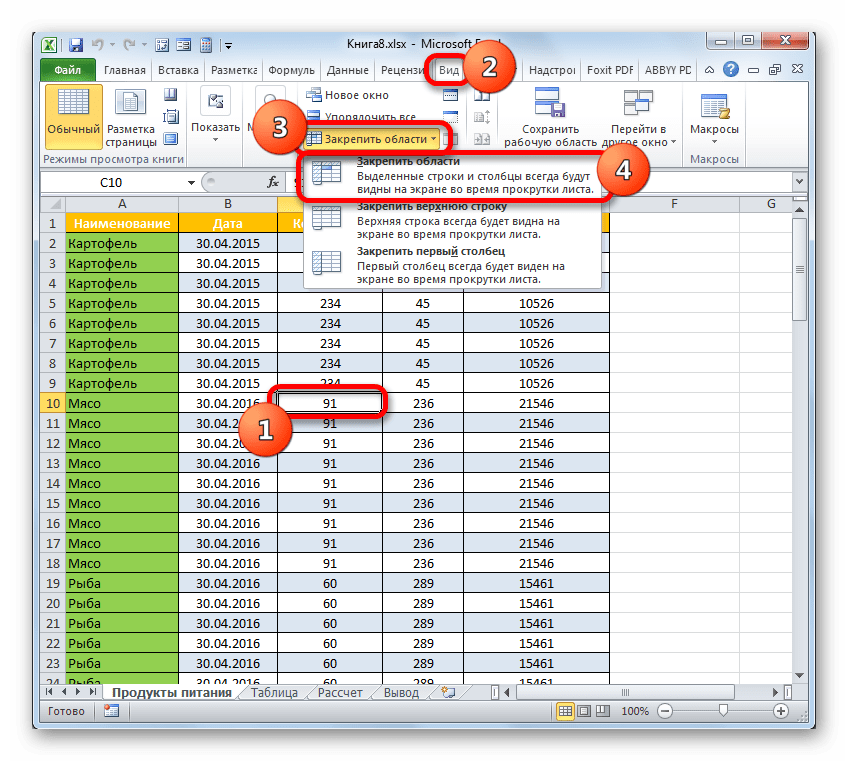
- Make any of the cells active. Go to the “VIEW” tab using the tool “Freeze Panes”.
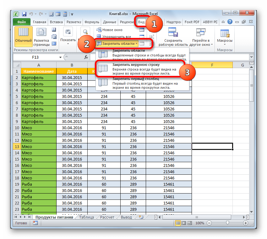
- In the menu select the “Freeze Top Row” functions.
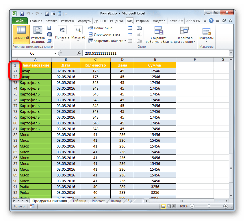
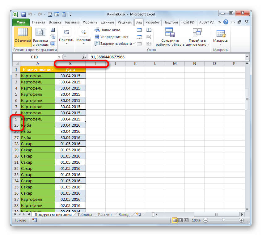
You will get a delimiting line under the top line. Now when you scroll vertically the table cap will be always visible.
Let us suppose, a user needs to fix not only the cap. For instance, another row or even a couple of rows must be fixed when scrolling the document. Doing it is possible and easy, when you follow these steps:
- Select any cell under the line, which we will fix. This action will help Excel to “understand”, which area should be fixed;
- Now select the “Freeze Panes” tool.
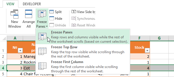
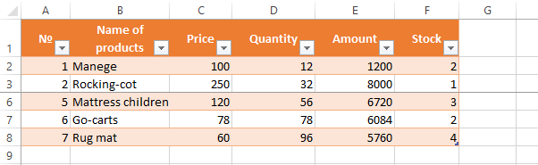
When you perform horizontal and vertical scrolling, the cap and the top row of the table remain fixed. Thus, you can fix two, three, four and more rows.
Note: This method works for 2007 and 2010 Excel versions. In earlier versions the “Lock areas” tool is located in the “Window” menu on the main page. There you must always (!) activate the cell under the freeze row.
Freezing columns in Excel
For instance, the information in the table has a horizontal direction. It is not concentrated in columns, but located in rows. For his comfort, the user must freeze the first column, containing the lines’ names in horizontal scrolling.
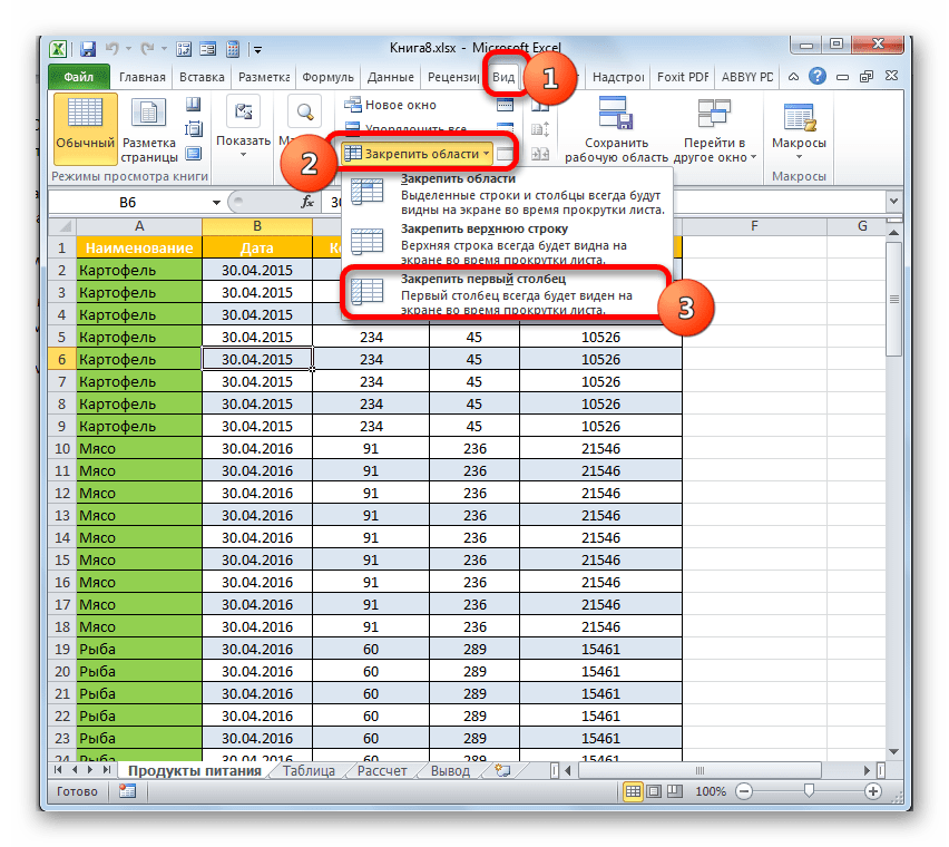
- Select any cell of the chosen table so that Excel understands with what data it will work. Pin the first column in the menu you will see..
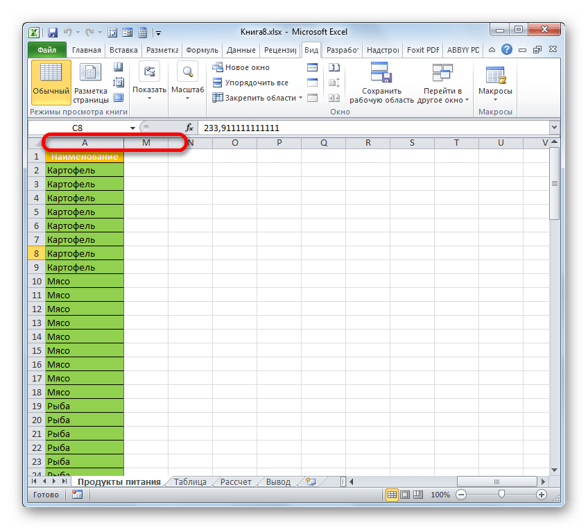
- Now, when the document is scrolled to the right horizontally, the needed column will be fixed.
To freeze several columns, select the cell at the page bottom (to the right from the fixed column). Pick the “Freeze Panes” button.
How to freeze the row and column in Excel
You have a task – to freeze the selected area, which contains two columns and two rows.
Make a cell at the intersection of the fixed rows and columns active. However, the cell must be not placed in the fixed area. It should have the position right under the required lines (to the right of the required columns). Pick the first option in Excel Locking Areas. The photo shows that when scrolling, the selected areas remain at the same place.
Removing a fixed area in Excel
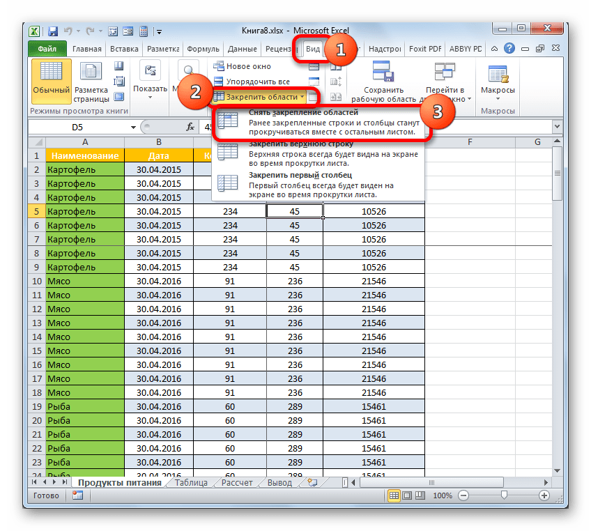
After fixing a row or a column of the table the button deleting all pivot tables becomes available.
After clicking – «Unfreeze Panes», all the locked areas of the worksheet become unlocked.
Источник
How to freeze rows and columns in Excel
 by Svetlana Cheusheva, updated on March 16, 2023
The tutorial shows how to freeze cells in Excel to keep them visible while you navigate to another area of the worksheet. Below you will find the detailed steps on how to lock a row or multiple rows, freeze one or more columns, or freeze column and row at once.
When working with large datasets in Excel, you may often want to lock certain rows or columns so that you can view their contents while scrolling to another area of the worksheet. This can be easily done by using the Freeze Panes command and a few other features of Excel.
How to freeze rows in Excel
Freezing rows in Excel is a few clicks thing. You just click View tab > Freeze Panes and choose one of the following options, depending on how many rows you wish to lock:
- Freeze Top Row — to lock the first row.
- Freeze Panes — to lock several rows.
The detailed guidelines follow below.
How to freeze top row in Excel
To lock top row in Excel, go to the View tab, Window group, and click Freeze Panes > Freeze Top Row.
This will lock the very first row in your worksheet so that it remains visible when you navigate through the rest of your worksheet. 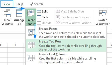
You can determine that the top row is frozen by a grey line below it: 
How to freeze multiple rows in Excel
In case you want to lock several rows (starting with row 1), carry out these steps:
- Select the row (or the first cell in the row) right below the last row you want to freeze.
- On the View tab, click Freeze Panes >Freeze Panes.
For example, to freeze top two rows in Excel, we select cell A3 or the entire row 3, and click Freeze Panes: 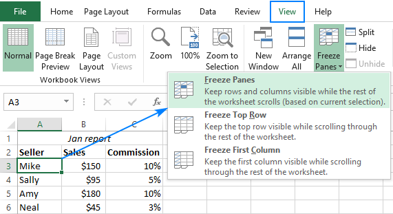
As the result, you’ll be able to scroll through the sheet content while continuing to view the frozen cells in the first two rows: 
- Microsoft Excel allows freezing only rows at the top of the spreadsheet. It is not possible to lock rows in the middle of the sheet.
- Make sure that all the rows to be locked are visible at the moment of freezing. If some of the rows are out of view, such rows will be hidden after freezing. For more information, please see How to avoid frozen hidden rows in Excel.
How to freeze columns in Excel
Freezing columns in Excel is done similarly by using the Freeze Panes commands.
How to lock the first column
To freeze the first column in a sheet, click View tab > Freeze Panes > Freeze First Column.
This will make the leftmost column visible at all times while you scroll to the right. 
How to freeze multiple columns in Excel
In case you want to freeze more than one column, this is what you need to do:
- Select the column (or the first cell in the column) to the right of the last column you want to lock.
- Go to the View tab, and click Freeze Panes >Freeze Panes.
For example, to freeze the first two columns, select the whole column C or cell C1, and click Freeze Panes: 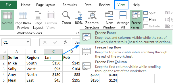
This will lock the first two columns in place, as indicated by the thicker and darker border, enabling you to view the cells in frozen columns as you move across the worksheet: 
- You can only freeze columns on the left side of the sheet. Columns in the middle of the worksheet cannot be frozen.
- All the columns to be locked should be visible, any columns that are out of view will be hidden after freezing.
How to freeze rows and columns in Excel
Besides locking columns and rows separately, Microsoft Excel lets you freeze both rows and columns at the same time. Here’s how:
- Select a cell below the last row and to the right of the last column you’d like to freeze.
- On the View tab, click Freeze Panes >Freeze Panes.
Yep, it’s that easy 🙂
For example, to freeze top row and first column in a single step, select cell B2 and click Freeze Panes: 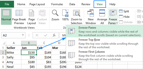
This way, the header row and leftmost column of your table will always be viewable as you scroll down and to the right: 
In the same fashion, you can freeze as many rows and columns as you want as long as you start with the top row and leftmost column. For instance, to lock top row and the first 2 columns, you select cell C2; to freeze the first two rows and the first two columns, you select C3, and so on.
How to unlock rows and columns in Excel
To unlock frozen rows and/or columns, go to the View tab, Window group, and click Freeze Panes > Unfreeze Panes. 
Freeze Panes not working
If the Freeze Panes button is disabled (greyed out) in your worksheet, most likely it’s because of the following reasons:
- You are in cell editing mode, for example entering a formula or editing data in a cell. To exit cell editing mode, press the Enter or Esc key.
- Your worksheet is protected. Please remove the workbook protection first, and then freeze rows or columns.
Other ways to lock columns and rows in Excel
Apart from freezing panes, Microsoft Excel provides a few more ways to lock certain areas of a sheet.
Split panes instead of freezing panes
Another way to freeze cells in Excel is to split a worksheet area into several parts. The difference is as follows:
Freezing panes allows you to keep certain rows or/and columns visible when scrolling across the worksheet.
Splitting panes divides the Excel window into two or four areas that can be scrolled separately. When you scroll within one area, the cells in the other area(s) remain fixed. 
To split Excel’s window, select a cell below the row or to the right of the column where you want the split, and click the Split button on the View tab > Window group. To undo a split, click the Split button again.
Use tables to lock top row in Excel
If you’d like the header row to always stay fixed at the top while you scroll down, convert a range to a fully-functional Excel table: 
The fastest way to create a table in Excel is by pressing the Ctl + T shortcut. For more information, please see How to make a table in Excel.
In case you’d like to repeat top row or rows on every printed page, switch to the Page Layout tab, Page Setup group, click the Print Titles button, go to the Sheet tab, and select Rows to repeat at top. The detailed instructions can be found here: Print row and column headers on every page.
That’s how you can lock a row in Excel, freeze a column, or freeze both rows and columns at a time. I thank you for reading and hope to see you on our blog next week!
Источник
Содержание
- Виды фиксации
- Способ 1: заморозка адреса
- Способ 2: закрепление ячеек
- Способ 3: защита от редактирования
- Вопросы и ответы

Эксель – это динамические таблицы, при работе с которыми сдвигаются элементы, меняются адреса и т.д. Но в некоторых случаях нужно зафиксировать определенный объект или, как по-другому говорят, заморозить, чтобы он не менял свое местоположение. Давайте разберемся, какие варианты позволяют это сделать.
Виды фиксации
Сразу нужно сказать, что виды фиксации в Экселе могут быть совершенно различные. В общем, их можно разделить на три большие группы:
- Заморозка адреса;
- Закрепление ячеек;
- Защита элементов от редактирования.
При заморозке адреса ссылка на ячейку не изменяется при её копировании, то есть, она перестает быть относительной. Закрепление ячеек позволяет их видеть постоянно на экране, как бы далеко пользователь не прокручивал лист вниз или вправо. Защита элементов от редактирования блокирует любые изменения данных в указанном элементе. Давайте подробно рассмотрим каждый из этих вариантов.
Способ 1: заморозка адреса
Вначале остановимся на фиксации адреса ячейки. Чтобы его заморозить, из относительной ссылки, каковой является любой адрес в Эксель по умолчанию, нужно сделать абсолютную ссылку, не меняющую координаты при копировании. Для того, чтобы сделать это, нужно установить у каждой координаты адреса знак доллара ($).
Установка знака доллара совершается нажатием на соответствующий символ на клавиатуре. Он расположен на одной клавише с цифрой «4», но для выведения на экран нужно нажать данную клавишу в английской раскладке клавиатуры в верхнем регистре (с зажатой клавишей «Shift»). Существует и более простой и быстрый способ. Следует выделить адрес элемента в конкретной ячейке или в строке функций и нажать на функциональную клавишу F4. При первом нажатии знак доллара появится у адреса строки и столбца, при втором нажатии на данную клавишу он останется только у адреса строки, при третьем нажатии – у адреса столбца. Четвертое нажатие клавиши F4 убирает знак доллара полностью, а следующее запускает данную процедуру по новому кругу.
Взглянем, как работает заморозка адреса на конкретном примере.
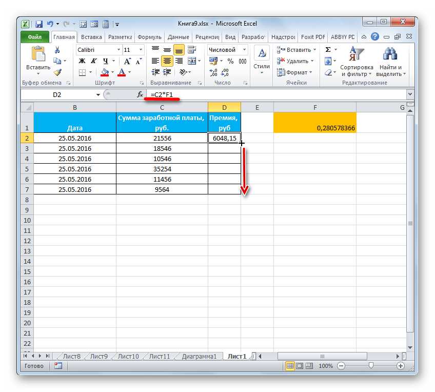
- Для начала скопируем обычную формулу в другие элементы столбца. Для этого воспользуемся маркером заполнения. Устанавливаем курсор в нижний правый угол ячейки, данные из которой нужно скопировать. При этом он трансформируется в крестик, который носит название маркера заполнения. Зажимаем левую кнопку мыши и тянем этот крестик вниз до конца таблицы.
- После этого выделяем самый нижний элемент таблицы и смотрим в строке формул, как изменилась формула во время копирования. Как видим, все координаты, которые были в самом первом элементе столбца, при копировании сместились. Вследствие этого формула выдает некорректный результат. Это связано с тем фактом, что адрес второго множителя, в отличие от первого, для корректного расчета смещаться не должен, то есть, его нужно сделать абсолютным или фиксированным.
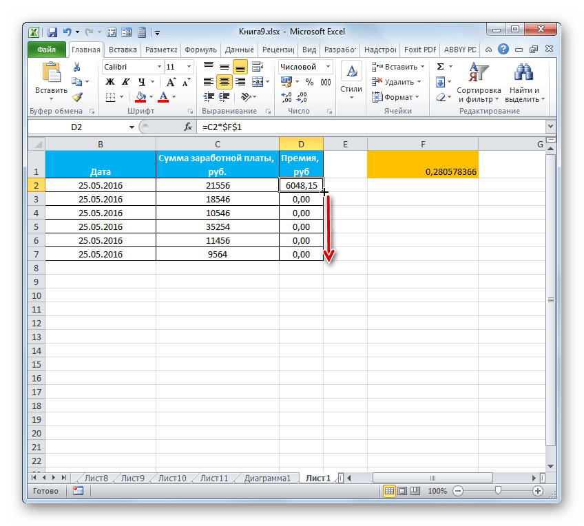
- Возвращаемся в первый элемент столбца и устанавливаем знак доллара около координат второго множителя одним из тех способов, о которых мы говорили выше. Теперь данная ссылка заморожена.
- После этого, воспользовавшись маркером заполнения, копируем её на диапазон таблицы, расположенный ниже.
- Затем выделяем последний элемент столбца. Как мы можем наблюдать через строку формул, координаты первого множителя по-прежнему смещаются при копировании, а вот адрес во втором множителе, который мы сделали абсолютным, не изменяется.
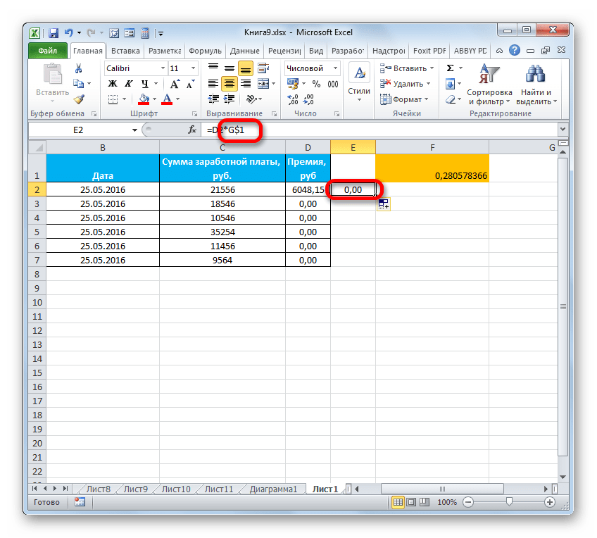
- Если поставить знак доллара только у координаты столбца, то в этом случае адрес столбца ссылки будет фиксированным, а координаты строки смещаются при копировании.
- И наоборот, если установить знак доллара около адреса строки, то при копировании он не будет смещаться, в отличие от адреса столбца.


Таким методом производится заморозка координат ячеек.

Урок: Абсолютная адресация в Экселе
Способ 2: закрепление ячеек
Теперь узнаем, как зафиксировать ячейки, чтобы они постоянно оставались на экране, куда бы пользователь не переходил в границах листа. В то же время нужно отметить, что отдельный элемент закрепить нельзя, но можно закрепить область, в которой он располагается.
Если нужная ячейка расположена в самой верхней строке листа или в левом крайнем его столбце, то закрепление провести элементарно просто.
- Для закрепления строки выполняем следующие действия. Переходим во вкладку «Вид» и клацаем по кнопке «Закрепить области», которая располагается в блоке инструментов «Окно». Открывается список различных вариантов закрепления. Выбираем наименование «Закрепить верхнюю строку».
- Теперь даже, если вы спуститесь на самый низ листа, первая строка, а значит и нужный вам элемент, находящийся в ней, будут все равно в самом верху окна на виду.
Аналогичным образом можно заморозить и крайний левый столбец.
- Переходим во вкладку «Вид» и жмем на кнопку «Закрепить области». На этот раз выбираем вариант «Закрепить первый столбец».
- Как видим, самый крайний левый столбец теперь закреплен.
Примерно таким же способом можно закрепить не только первый столбец и строку, но и вообще всю область находящуюся слева и сверху от выбранного элемента.
- Алгоритм выполнения данной задачи немного отличается от предыдущих двух. Прежде всего, нужно выделить элемент листа, область сверху и слева от которого будет закреплена. После этого переходим во вкладку «Вид» и щелкаем по знакомой иконке «Закрепить области». В открывшемся меню выбираем пункт с точно таким же наименованием.
- После данного действия вся область, находящаяся слева и выше выделенного элемента, будет закреплена на листе.
При желании снять заморозку, выполненную таким способом, довольно просто. Алгоритм выполнения одинаков во всех случаях, что именно пользователь не закреплял бы: строку, столбец или область. Перемещаемся во вкладку «Вид», щелкаем по иконке «Закрепить области» и в открывшемся списке выбираем вариант «Снять закрепление областей». После этого будут разморожены все закрепленные диапазоны текущего листа.
Урок: Как закрепить область в Excel
Способ 3: защита от редактирования
Наконец, можно защитить ячейку от редактирования, заблокировав в ней возможность вносить изменения для пользователей. Таким образом все данные, которые находятся в ней, будут фактически заморожены.
Если ваша таблица не является динамической и не предусматривает внесение в неё со временем каких-либо изменений, то можно защитить не только конкретные ячейки, но и весь лист в целом. Это даже значительно проще.
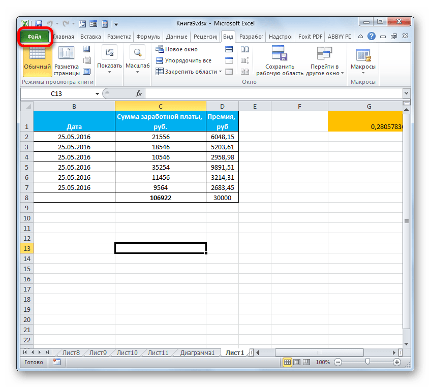
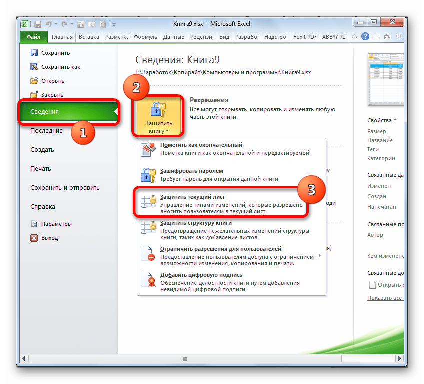
- Перемещаемся во вкладку «Файл».
- В открывшемся окне в левом вертикальном меню переходим в раздел «Сведения». В центральной части окна клацаем по надписи «Защитить книгу». В открывшемся перечне действий по обеспечению безопасности книги выбираем вариант «Защитить текущий лист».
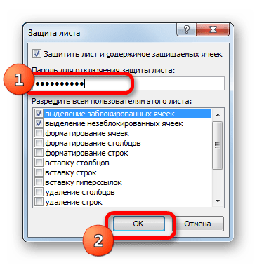
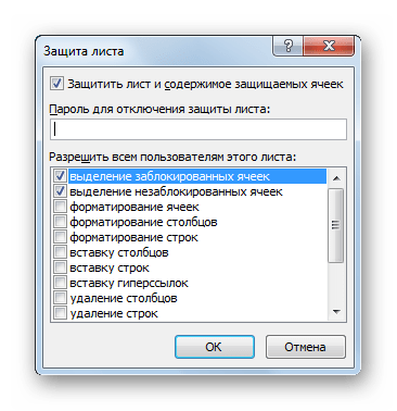
- Запускается небольшое окошко, которое называется «Защита листа». Прежде всего, в нем в специальном поле требуется ввести произвольный пароль, который понадобится пользователю, если он в будущем пожелает отключить защиту, чтобы выполнить редактирование документа. Кроме того, по желанию, можно установить или убрать ряд дополнительных ограничений, устанавливая или снимая флажки около соответствующих пунктов в перечне, представленном в данном окне. Но в большинстве случаев настройки по умолчанию вполне соответствуют поставленной задаче, так что можно просто после введения пароля клацать по кнопке «OK».
- После этого запускается ещё одно окошко, в котором следует повторить пароль, введенный ранее. Это сделано для того, чтобы пользователь был уверен, что ввел именно тот пароль, который запомнил и написал в соответствующей раскладке клавиатуры и регистре, иначе он сам может утратить доступ к редактированию документа. После повторного введения пароля жмем на кнопку «OK».
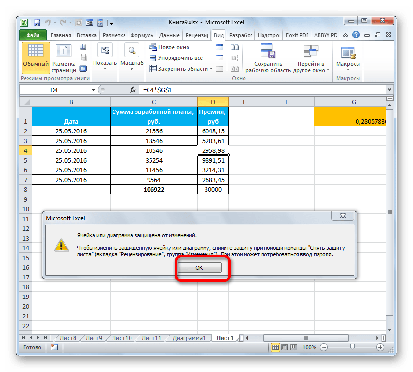
- Теперь при попытке отредактировать любой элемент листа данное действие будет блокировано. Откроется информационное окно, сообщающее о невозможности изменения данных на защищенном листе.

Имеется и другой способ заблокировать любые изменения в элементах на листе.
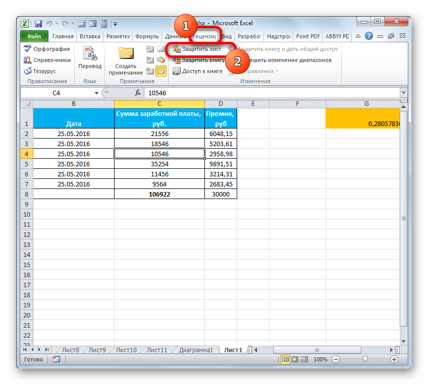
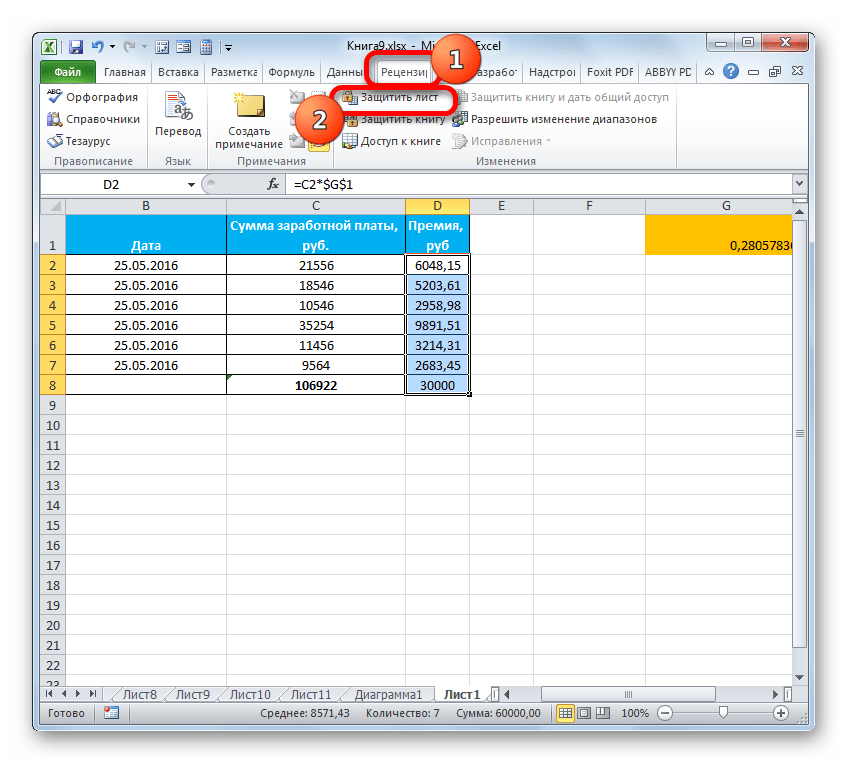
- Переходим в окно «Рецензирование» и клацаем по иконке «Защитить лист», которая размещена на ленте в блоке инструментов «Изменения».
- Открывается уже знакомое нам окошко защиты листа. Все дальнейшие действия выполняем точно так же, как было описано в предыдущем варианте.
Но что делать, если требуется заморозить только одну или несколько ячеек, а в другие предполагается, как и раньше, свободно вносить данные? Существует выход и из этого положения, но его решение несколько сложнее, чем предыдущей задачи.
Во всех ячейках документа по умолчанию в свойствах выставлено включение защиты, при активации блокировки листа в целом теми вариантами, о которых говорилось выше. Нам нужно будет снять параметр защиты в свойствах абсолютно всех элементов листа, а потом установить его заново только в тех элементах, которые желаем заморозить от изменений.
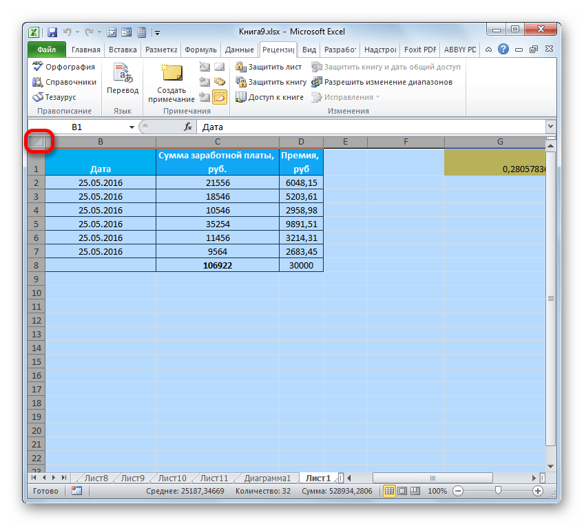
- Кликаем по прямоугольнику, который располагается на стыке горизонтальной и вертикальной панелей координат. Можно также, если курсор находится в любой области листа вне таблицы, нажать сочетание горячих клавиш на клавиатуре Ctrl+A. Эффект будет одинаковый – все элементы на листе выделены.
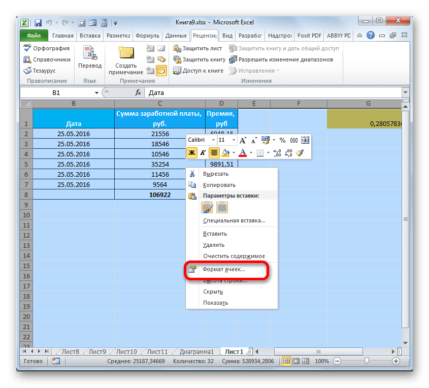
- Затем клацаем по зоне выделения правой кнопкой мыши. В активированном контекстном меню выбираем пункт «Формат ячеек…». Также вместо этого можно воспользоваться набором сочетания клавиш Ctrl+1.
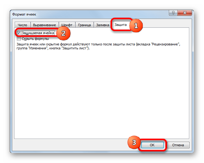
- Активируется окошко «Формат ячеек». Сразу же выполняем переход во вкладку «Защита». Тут следует снять флажок около параметра «Защищаемая ячейка». Щелкаем по кнопке «OK».
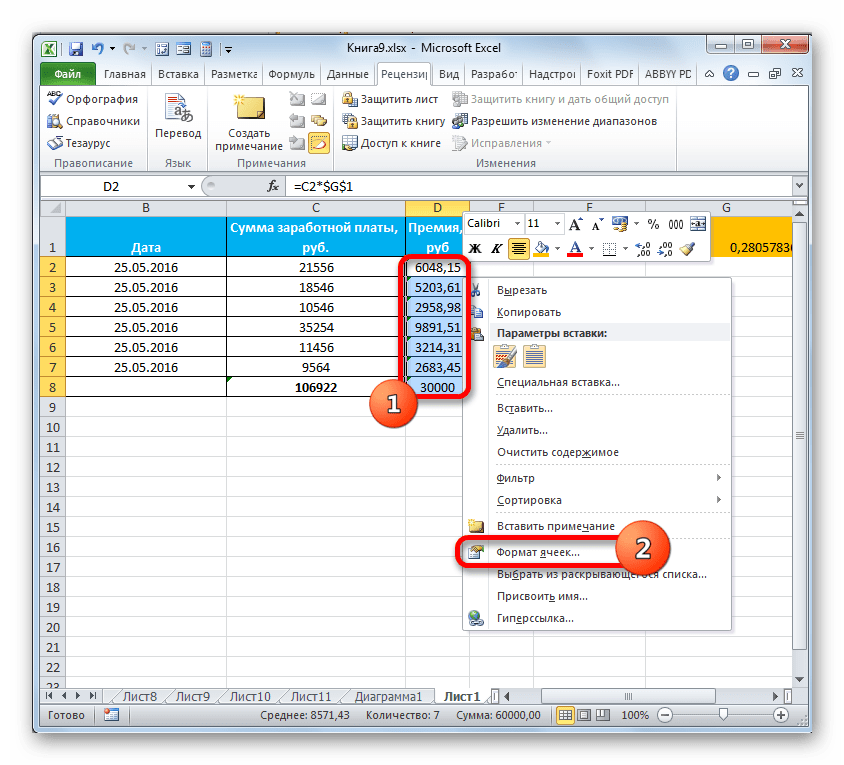
- Далее возвращаемся на лист и выделяем тот элемент или группу, в которой собираемся заморозить данные. Жмем правой кнопкой мыши по выделенному фрагменту и в контекстном меню переходим по наименованию «Формат ячеек…».
- После открытия окна форматирования в очередной раз переходим во вкладку «Защита» и ставим флажок возле пункта «Защищаемая ячейка». Теперь можно нажать на кнопку «OK».
- После этого устанавливаем защиту листа любым из тех двух способов, которые были описаны ранее.

После выполнения всех процедур, подробно описанных нами выше, заблокированными от изменений будут только те ячейки, на которые мы повторно установили защиту через свойства формата. Во все остальные элементы листа, как и прежде, можно будет свободно вносить любые данные.
Урок: Как защитить ячейку от изменений в Экселе
Как видим, существует сразу три способа провести заморозку ячеек. Но важно заметить, что отличается в каждом из них не только технология выполнения данной процедуры, но и суть самой заморозки. Так, в одном случае фиксируется только адрес элемента листа, во втором – закрепляется область на экране, а в третьем – устанавливается защита на изменения данных в ячейках. Поэтому очень важно понимать перед выполнением процедуры, что именно вы собираетесь блокировать и зачем вы это делаете.
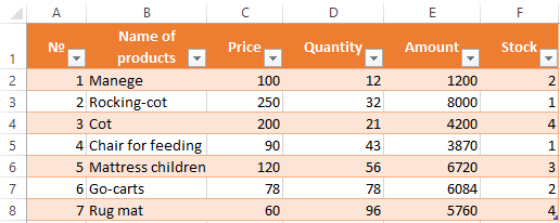
Surely you all know the Microsoft Excel application. Microsoft Excel is an application or software that is useful for processing numbers. As you already know, this application has a lot of uses and benefits.
The usefulness of this application is that it can create, analyze, edit, Rank, and sort several data because this application can calculate with arithmetic and statistics.
This tutorial will explain how to sort or rank data using Microsoft Excel.
How to Rank in Microsoft Excel
You can rank data in Microsoft Excel. By using the application, you can easily do work in processing data. Ranking data is also very useful for those who work as teachers.
Because this application can rank data in a very easy way and can be done by everyone. Here are ways to rank data in Microsoft Excel:
1. The first step you can take is to open a Microsoft Excel worksheet that already has the data you want to rank. In the example below, I want to rank students in a class by sorting them from rank 1 to 7 You can also rank according to the data you have.
![]()
2. After that, you can place your cursor in the cell, where you will rank the cells in the first order. You can see an example in the image below.
![]()
After that, you can write a formula to rank in Microsoft Excel in the fx column. And here’s the formula, =rank(number;ref;order) .
The meaning of the formula is = Rank Rank, which means it is a rank function. And (number; ref; order) means the initial cell number that has a value to be ranked, its reference, and the final cell number that has a value to be ranked, the reference.
The formula is =Rank(D3;$D$3:$D$9;0) in the example below. After entering the function, you can press the Enter key on your keyboard. And here are the results, namely the ranking on data number 1, which has a ranking of 1.
![]()
3. If you want to do the same thing to all data as in data number 1, you have to copy the previous column, and then you can block the column below it and click Paste. Then you can see the results. All the columns in the Rank entity have been ranked in such away.
![]()
4. The results above are not satisfactory because the data is still not sorted, so it looks messy. We must make it sequentially according to the ranking from the smallest to the largest, and this example must be sorted from rank 1 to rank 9.
The way to sort it is to block the contents of all tables, but not with the column names and the contents of the column number.
![]()
5. After that, you can do the sorting by going to the Editing tool, clicking Sort & Filter, and then clicking the Custom Sort option…
![]()
6. Then the Sort box will appear, where you have to choose sort by with the Rank option, some kind on with the Values option, and order with the Smallest to Largest option. After that, you can click OK.
7. Below is the result of the sorting we have done above. In this way, the data that has been ranked will be sorted according to its ranking.
![]()
That’s the tutorial on how to rank using Microsoft Excel. Hopefully, this article can be useful for you.
A large table with tons of data usually can’t be fully displayed in a single page. You must scroll down or scroll to the right for a more complete viewing. In order to correspond these data with the title or other key content intuitively, you can freeze some specified cells in the table. In this way, even when you scroll down the page, the selected content will always show at the top of the page.
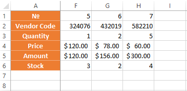
How to Freeze Top Row and First Column in Excel
1. Switch to View tab in Excel, find the feature called Freeze Panes in the Window section.

2. Click it, there are two common used options: Freeze Top Row and Freeze First Column. As their name suggest, you can simply freeze the first row or the first column in the table by selecting them.

If you want to freeze a specified area of cells, you’d better make use of the feature Freeze Panes.
Freeze Panes allows you to freeze a specified range of cells, but not in a direct way. When you click a cell, the intersection of cells above it and cells on the left of it will be specified as the panes to freeze. For example, when I click D2 in the table and select Freeze Panes, the cells from A1 to C1 will be frozen. You can see the black borders around them which delimits the scope of cells to be frozen.

Now when I scroll down the page, the cells above the horizontal border line will always stay at the top of the sheet; When I scroll to the right, the cells on the left of the vertical border line will always stay at the leftmost of the sheet. And no matter I scroll down or scroll to the right of the page, cell A1, B1 and C1 will always stay at the same place.

How to Unfreeze Panes in Excel
If you don’t want to freeze these cells anymore, just click Freeze Panes again and choose Unfreeze Panes in the drop-down list.

Copyright Statement: Regarding all of the posts by this website, any copy or use shall get the written permission or authorization from Myofficetricks.
Just assume you are school teacher and have around 90 students in a class which is divided into various sections. Now, you have to collate their marks in every subject in an excel.
If you are using a 15-inch laptop to do this, then as soon as you go to the 25th row or later you lose the context of which column is for which subject. All of this happens because your header or first row is not fixed and keeps changing as you scroll down. But don’t worry we are here to help you out. 🙂
In this post we are going to help you on how to freeze rows or columns in excel. Freeing in excel will turn some cells (rows and / or columns) to be stagnant and these cells would not change if you move left or right or scroll up or down. There are various ways to freeze cells in excel.

We have listed all the methods below, if you do not want to go through the entire post then you may directly click on the type of excel freeze option you are looking for:
- Freeze First Row
- Freeze First Column
- Freeze Panes
- Freeze Multiple Rows
- Freeze Multiple Columns
- Freeze Rows & Columns at same time
Along with helping you on how to freeze in excel, we will also help you to unfreeze and troubleshooting issues that you might encounter:
- Unfreeze Panes
- Freeze panes versus Splitting Panes
- Freeze Pane is Disabled
Freeze First Row
This feature could be used to freeze a particular row or header that you would need to refer every time while working on excel. In this option only the top row will freeze.
- Open the sheet where in you want to freeze any row / header, as an example we would like to freeze the top row highlighted in yellow

- Now, navigate to the “View” tab in the Excel Ribbon as shown in above image
- Click on the “Freeze Panes” button

- Select “Freeze Top Row” option

- If you would like to freeze any other row, then scroll down and make that row appear as first in your sheet and then repeat Step 2 to 4.
That’s it. You are all set now. As seen in above image you can now scroll to any corner of the page and you would see that the top row remains intact all the time without any change.
Please note that this option works as long as first row in excel is the one that you really want to freeze. If you have scrolled in the middle of the sheet and Row 30 is appearing as first row, then this option would freeze Row 30 and not Row 1.
Additionally, if you are geek and would like to do it directly using a keyboard shortcut, then please press “Alt + W” followed by “F” and then “R”. Please note that this is not an in-built shortcut, rather it’s the same thing from keyboard as we do from mouse.
Freeze First Column
This feature could be used to freeze a particular column that you would need to refer while working on excel. In this option only the first column will freeze.
- Open the sheet where in you want to freeze the column, as an example we would like to freeze the column A – Product

- Now, navigate to the “View” tab in the Excel Ribbon as shown in above image
- Click on the “Freeze Panes” button

- Select “Freeze First Column” option

- If you would like to freeze any other column, then move right or left and make that column appear as first in your sheet and then repeat Step 2 to 4.
That’s it. You are all set now. As seen in above image you can now move to most right corner of the page and you would see that the first column sticks there. Please note that this option works as long as first column in excel is the one that you really want to freeze. If you have shifted right in the middle of the sheet and Column M is appearing as first row, then this option would freeze Column M and not Column A.
If you would like to do it directly using a keyboard shortcut, then please press “Alt + W” followed by “F” and then “C”. Please note that this is not an in-built shortcut, rather it’s the same thing from keyboard as we do from mouse.
Freeze Panes
This feature could be used to freeze multiple rows, columns or both at the same time. However, this could be done only for the consecutive rows or columns.
Freeze Panes – Multiple Rows
- Open the sheet where in you want to freeze the multiple rows, keep the first row on top and click after the last row till where you want to freeze, as an example we would like to freeze from Row 1 to Row 13 so we will click on Row 14

- Now, navigate to the “View” tab in the Excel Ribbon as shown in above image
- Click on the “Freeze Panes” button

- Select “Freeze Panes” option

That’s it. You are all set now. As seen in above image you can now scroll down and Row 1 to Row 13 will be kept intact without any changes. You can select the range of rows from middle as well like – Row 13 to Row 30, however to do so you will have to ensure that you scroll up and keep Row 13 as your first row in the sheet and repeat the steps listed above. However, be careful as doing so some of your rows (i.e. the ones before Row 13) will be hidden.
Freeze Panes – Multiple Columns
- Open the sheet where in you want to freeze the multiple columns, keep the first column to the left and click next to the last column till where you want to freeze, as an example we would like to freeze from Column A to E, so we will click on Column F

- Now, navigate to the “View” tab in the Excel Ribbon as shown in above image
- Click on the “Freeze Panes” button

- Select “Freeze Panes” option

That’s it. You are all set now. As seen in above image you can now move towards right and Column A to E will be kept intact without any changes. You can select the range of columns from middle as well like – Column F to Column L, however to do so you will have to ensure that you move to the left and keep Column F as your first column in the sheet and repeat the steps listed above. However, be careful as doing so some of your columns (i.e. the ones before Column E) will be hidden.
Freeze Panes – Multiple Rows and Columns both
If you have followed the post till now, then you would have already figured out how this has to be done. Yes, you are right we are going to club both the above listed approaches here. Follow us below:
- Open the sheet where in you want to freeze the multiple rows and columns, keep the first row on top and first column to the left then click next to the cell of the last column and row till where you want to freeze, as an example we would like to freeze from Row 1 to 13 and Column A to E, so we will click on Cell F14

- Now, navigate to the “View” tab in the Excel Ribbon as shown in above image
- Click on the “Freeze Panes” button

- Select “Freeze Panes” option

That’s it. You are all set now. As seen in above image you can now scroll down and Row 1 to 13 will remain intact and likewise you can move towards right and Column A to E will be kept intact without any changes. You can select the range of columns from middle as well like – Row 17 to 27 and Column F to L, however to do so you will have to ensure that you scroll up and keep Row 17 as your first row and keep Column F as your first column in the sheet and repeat the steps listed above. Be careful here as rows before Row 17 and columns before column F will be hidden.
Unfreeze Panes:
If you have frozen the wrong rows and columns, then you could easily undo it by using “Unfreeze Panes” option. This would remove all the frozen rows and or columns in your excel. This will also work if you have received the sheet from someone else and you are not able to see all the rows and columns despite of removing all filters and unhiding rows columns. To unfreeze panes –
- Open the sheet wherein you want to unfreeze rows and or columns
- Now, navigate to the “View” tab in the Excel Ribbon
- Click on the “Freeze Panes” button

- Select “Unfreeze Panes” option as shown above

With this all the rows and or columns would unfreeze, as shown in above image. Please note that you would not see the “Unfreeze Panes” option if there are not any frozen rows columns. This option would be available only and only when there is some row and or column frozen already.
If you would like to unfreeze panes it directly using a keyboard shortcut, then please press “Alt + W” followed by “F” and then again “F”. Please note that this is not an in-built shortcut, rather it’s the same thing from keyboard as we do from mouse.
Freeze panes versus Splitting Panes:
Excel also provides you an excellent option to Split Panes which divides the window into different panes that each pane scrolls separately. This option is present in Excel Ribbon, View tab next to Freeze Option.

So as visible in the above image after using split option the content of same sheet is visible in 4 separate panes and all panes have their different scroll options.
We personally trust and use Freeze option much than Split, as Freeze allows you to limit the data movement by freezing it rather than adding multiple views of same data wherein you easily get distracted and confused while data entry.
Is Freeze Pane option disabled?
If you have come across a case wherein the Freeze Pane option is disabled in your sheet, then it must be due to one of the following reasons:
- The most common reason of Freeze Panes option disablement is that your sheet must have been opened in “Page Layout” mode (as shown in below image)

In order to correct it simply navigate to “View Tab” in the excel ribbon and select “Normal” or “Page Break” view.
- The “Freeze Panes” option could also be disabled if you excel has been protected for windows. You would need to unprotect it to enable the freeze option.
So, this was all about how to freeze rows and columns in Excel. Hope you enjoyed our tutorial. Please feel free to share your feedback and queries. Keep Exceling 🙂