
Add or subtract days from a date
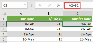
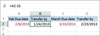
Suppose that a bill of yours is due on the second Friday of each month. You want to transfer funds to your checking account so that those funds arrive 15 calendar days before that date, so you’ll subtract 15 days from the due date. In the following example, you’ll see how to add and subtract dates by entering positive or negative numbers.
-
Enter your due dates in column A.
-
Enter the number of days to add or subtract in column B. You can enter a negative number to subtract days from your start date, and a positive number to add to your date.
-
In cell C2, enter =A2+B2, and copy down as needed.
Add or subtract months from a date with the EDATE function
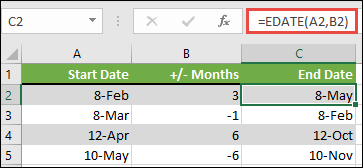
You can use the EDATE function to quickly add or subtract months from a date.
The EDATE function requires two arguments: the start date and the number of months that you want to add or subtract. To subtract months, enter a negative number as the second argument. For example, =EDATE(«9/15/19»,-5) returns 4/15/19.
-
For this example, you can enter your starting dates in column A.
-
Enter the number of months to add or subtract in column B. To indicate if a month should be subtracted, you can enter a minus sign (-) before the number (e.g. -1).
-
Enter =EDATE(A2,B2) in cell C2, and copy down as needed.
Notes:
-
Depending on the format of the cells that contain the formulas that you entered, Excel might display the results as serial numbers. For example, 8-Feb-2019 might be displayed as 43504.
-
Excel stores dates as sequential serial numbers so that they can be used in calculations. By default, January 1, 1900 is serial number 1, and January 1, 2010 is serial number 40179 because it is 40,178 days after January 1, 1900.
-
If your results appear as serial numbers, select the cells in question and continue with the following steps:
-
Press Ctrl+1 to launch the Format Cells dialog, and click the Number tab.
-
Under Category, click Date, select the date format you want, and then click OK. The value in each of the cells should appear as a date instead of a serial number.
-
-
Add or subtract years from a date
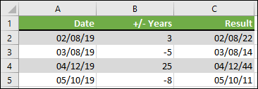
In this example, we’re adding and subtracting years from a starting date with the following formula:
=DATE(YEAR(A2)+B2,MONTH(A2),DAY(A2))
How the formula works:
-
The YEAR function looks at the date in cell A2, and returns 2019. It then adds 3 years from cell B2, resulting in 2022.
-
The MONTH and DAY functions only return the original values from cell A2, but the DATE function requires them.
-
Finally, the DATE function then combines these three values into a date that’s 3 years in the future — 02/08/22.
Add or subtract a combination of days, months, and years to/from a date
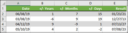
In this example, we’re adding and subtracting years, months and days from a starting date with the following formula:
=DATE(YEAR(A2)+B2,MONTH(A2)+C2,DAY(A2)+D2)
How the formula works:
-
The YEAR function looks at the date in cell A2, and returns 2019. It then adds 1 year from cell B2, resulting in 2020.
-
The MONTH function returns 6, then adds 7 to it from cell C2. This gets interesting, because 6 + 7 = 13, which is 1-year and 1-month. In this case, the formula will recognize that and automatically add another year to the result, bumping it from 2020 to 2021.
-
The DAY function returns 8, and adds 15 to it. This will work similarly to the MONTH portion of the formula if you go over the number of days in a given month.
-
The DATE function then combines these three values into a date that is 1 year, 7 months, and 15 days in the future — 01/23/21.
Here are some ways you could use a formula or worksheet functions that work with dates to do things like, finding the impact to a project’s schedule if you add two weeks, or time needed to complete a task.
Let’s say your account has a 30-day billing cycle, and you want to have the funds in your account 15 days before the March 2013 billing date. Here’s how you would do that, using a formula or function to work with dates.
-
In cell A1, type 2/8/13.
-
In cell B1, type =A1-15.
-
In cell C1, type =A1+30.
-
In cell D1, type =C1-15.

Add months to a date
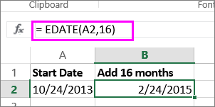
We’ll use the EDATE function and you’ll need the start date and the number of months you want to add. Here’s how to add 16 months to 10/24/13:
-
In cell A1, type 10/24/13.
-
In cell B1, type =EDATE(A1,16).
-
To format your results as dates, select cell B1. Click the arrow next to Number Format, > Short Date.
Subtract months from a date
We’ll use the same EDATE function to subtract months from a date.
Type a date in Cell A1 and in cell B1, type the formula =EDATE(4/15/2013,-5).
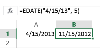
Here, we’re specifying the value of the start date entering a date enclosed in quotation marks.
You can also just refer to a cell that contains a date value or by using the formula =EDATE(A1,-5)for the same result.
More examples
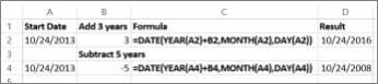
To add years to or subtract years from a date
|
Start Date |
Years added or subtracted |
Formula |
Result |
|---|---|---|---|
|
10/24/2013 |
3 (add 3 years) |
=DATE(YEAR(A2)+B2,MONTH(A2),DAY(A2)) |
10/24/2016 |
|
10/24/2013 |
-5 (subtract 5 years) |
=DATE(YEAR(A4)+B4,MONTH(A4),DAY(A4)) |
10/24/2008 |
The DATE function in Excel is a date and time function representing the number provided to it as arguments in a date and time code. The arguments it takes are integers for a day, month, and year separately and give us the result in a simple date. The result displayed is in date format, but the arguments are provided as integers. Therefore, we can use the formula: =DATE( Year, Month, Day) on a sequential basis.
For example, = DATE(2020,5,1) equals May 1, 2020.
Table of contents
- DATE Function in Excel
- DATE Formula for Excel
- How to Use the DATE Function in Excel? (with Examples)
- Example #1 – Get a month from the date
- Example #2 – Find out a leap year
- Example #3 – Highlight a set of dates
- Things to Remember
- Usage of DATE Function in Excel VBA
- DATE function in VBA Example
- DATE Excel Function Video
- Recommended Articles
DATE Formula for Excel
The DATE formula for Excel is as follows:

The DATE formula for Excel has three arguments, out of which two are optional. When,
- year = The year to use while creating the date.
- month = The month to use while creating the date.
- day = The day to use while creating the date
How to Use the DATE Function in Excel? (with Examples)
The DATE is a Worksheet (WS) function. It can be entered as a part of the formula in a worksheet cell as a WS function. You may refer to the DATE function examples given below to understand better.
You can download this DATE Function Excel Template here – DATE Function Excel Template
Example #1 – Get a month from the date
MONTH(DATE(2018,8,28))
As shown in the above DATE formula, the MONTH function is applied on the date represented using the DATE function. The MONTH function will return the month index produced by the DATE function. E.g., 8 in the given example. Cell D2 has a DATE formula, hence the result ‘8’.

Example #2 – Find out a leap year
MONTH(DATE(YEAR(B3),2,29)) = 2
As shown in the above DATE formula, the DATE will automatically adjust to month and year values out of range. Here, the innermost formula is YEAR with parameters as cell B3 indicating the input data, 2 is the index of February month, and 29 for the day. For example, February has 29 days in leap years, so the outer DATE function will return the output as 2/29/2000.
In case of a non-leap year, DATE will return the date March 1 of the year because there is no 29th day, and DATE would roll the date forward into the next month.
The outermost function, MONTH, would extract the month from the result. E.g., 2 or in case of a leap year and 3 in case of a non-leap year.
Further, the result is compared with a constant ‘2’. For example, if the month is 2, the DATE formula in excel returns “TRUE.” If not, the DATE formula returns “FALSE.”
In the following screenshot, cell B2 contains a date belonging to a leap year, and B3 has a date belonging to a non-leap year.

Example #3 – Highlight a set of dates
A conditional formattingA complementary good is one whose usage is directly related to the usage of another linked or associated good or a paired good i.e. we can say two goods are complementary to each other. read more rule is applied to column B in this DATE function example. The dates greater than 2005/1/1 are highlighted using a pink color style. So, as shown in the screenshot, three dates greater than the specified date are highlighted in the configured format. The other two dates that do not satisfy the criteria are left unformatted as no rule applies to such dates.

Things to Remember
- The Excel DATE function returns a date serial number. One must format the result as a date to display the date format.
- If the year is between 0 and 1900, Excel will add 1900 to the year.
- A month can be greater than 12 and less than zero. If the month is greater than 12, Excel will add a month to the first month in the specified year. If the month is less than or equal to zero, Excel will subtract the absolute value of the month plus 1 (i.e., ABS(month) + 1) from the first month of the specified year.
- The day can be positive or negative. If a day is greater than the days in the specified month, Excel will add a day to the first day of the specified month. If a day is less than or equal to zero, Excel will subtract the absolute value of the day plus 1 (i.e., ABS(day) + 1) from the first day of the specified month.
Usage of DATE Function in Excel VBA
The DATE function in VBA returns the current system date. It can be used in Excel VBA as follows:

DATE function in VBA Example
Date()
Result: 12/08/2018
Here, the Date() function returns the current system date. The same can be assigned to a variable as follows:
Dim myDate As String
myDate = Date()
So, myDate = 12/08/2018
DATE Excel Function Video
Recommended Articles
This article has been a guide to the DATE Function in Excel. Here, we discuss the DATE formula for Excel and how to use the DATE function and Excel example, and downloadable Excel templates. You may also look at these useful functions in Excel:-
- VBA Excel Date
- Inserting Date in Excel
- DAY in Excel
- WEEKDAY Function
If you use Excel regularly, I’m sure you’ve come across dates and times in your cells. Data often has a record of when it was created or updated, so knowing how to work with this data is essential.
Here are three key skills that you’ll learn in this tutorial:
- How to format dates in Excel so that they appear in your preferred style
- Formulas to calculate the number of days, months, and years between two dates
- An Excel date formula to log today’s date, and a keyboard shortcut to add the current time
Microsoft Excel can basically do anything with data, if you just know how. This tutorial is another key step to adding skills to your Excel toolbelt. Let’s get started.
Excel Date and Time Formulas (Quick Video Tutorial)
This screencast will walk you through how to work with dates and times in Excel. I cover formatting dates to different styles, as well as Excel date formulas to calculate and work with dates. Make sure to download the free Excel workbook with exercises that I’ve attached to this tutorial.
Keep reading for a written reference guide on how to format dates and times in Excel, and work with them in your formulas. I’ll even share several tips that weren’t covered in the screencast.
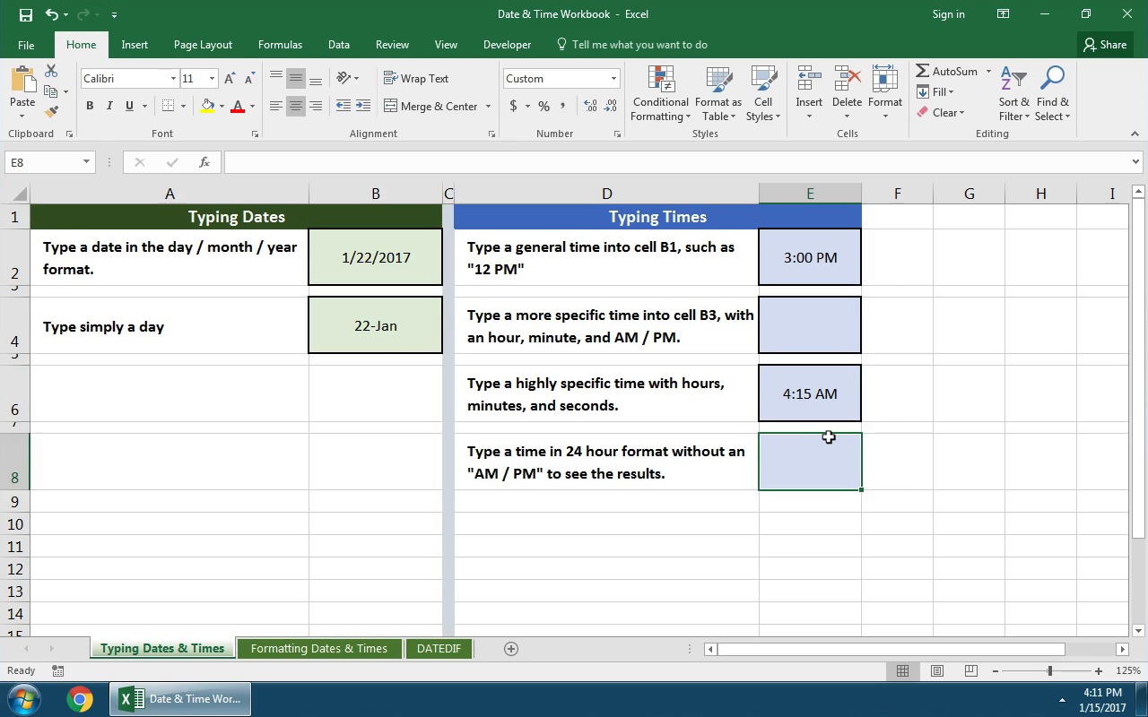
Typing Dates and Times in Excel
For this part of the tutorial, use the tab titled «Typing Dates & Times» in the example workbook.
One of the keys to working with dates and times in Excel is capturing the data correctly. Here’s how to type dates and times in your Excel spreadsheets:
1. How to Type Dates
I recommend typing dates in the same format that your system uses. For our American readers, a full date would be in the «day/month/year» format. European style dates are «month/day/year.»


When I’m typing dates, I always type in the full date with the month, day and year. If I only want to show the month and the year, I’ll simply format it that way (more on that in a minute.)
2. How to Type Times
It’s easy to type times in Excel. We can specify anything from just an hour of the day, to the exact second that something took place.
If I wanted to log the time as 4PM, I’d type «4 pm» into a cell in Excel and then press enter:


Notice once we press enter, Excel converts what we’ve typed into a hours : minutes: seconds data format.
Here’s how to log a more specific time in your spreadsheet:


The key is to use colons to separate the section of the time data, and then add a space plus «AM» or «PM.»
3. How to Type Date-Time Together
You can also type combinations of dates and times in Excel for highly specific timestamps.
To type a date-time combination, simply use what we’ve already learned about typing dates, and typing times.


Notice that Excel has converted the time to a 24 hour format when it’s used in conjunction with a date, by default. If you want to change the style of this date, keep reading.
Bonus: Excel Keyboard Shortcut for Current Time
One of my favorite Excel keyboard shortcuts inserts the current time into a spreadsheet. I use this formula often, when I’m noting the time I made a change to my data. Try it out:
Control + Shift + ;
Formatting Dates in Excel
For this part of the tutorial, use the tab titled «Formatting Dates & Times» in the example workbook.
What can you do when your dates are European style dates? That is, they’re in a day-month-year format, and you need to convert them to the more familiar month-day-year format?

In the screenshot above, what might surprise you is that all six of those cells contain exactly the same data — «1/22/2017.» What differs is how they’re formatted in Excel. The original data is identical, but it can be formatted to show in a variety of ways.
In most cases, it’s better to use formatting to modify the style of our dates. We don’t need to modify the data itself — just change how it’s presented.
Format Excel Cells
To change the appearance of our date and time data, make sure that you’re working on the Home tab of Excel. On the Ribbon (menu at the top of Excel), find the section labeled Number.
There’s a small arrow in the lower right corner of the section. Click it to open the Format Cells menu.


The Format Cells menu has a variety of options for styling your dates and times. You could turn «1/22/2017» into «Sunday, January 22nd» with just formatting. Then, you could grab the format painter and change all of your cell styles.


Spend some time exploring this menu and trying out the different styles for your Excel dates and times.
Get Data From Dates and Times
Let’s say that we have a list of data that has very specific dates and times, and we want to get simpler versions of those formulas. Maybe we have a list of exact transaction dates, but we want to work with them at a higher level, grouping them by year or month.
You can get the year from a date with this Excel formula:
=YEAR(CELL)


To get just the month from a date cell, use the following Excel formula:
=MON(CELL)


Find the Difference Between Dates and Times
For this part of the tutorial, use the tab titled «DATEDIF» in the example workbook.
While formats are used to change how dates and times are presented, formulas in Excel are used to modify, calculate, or work with dates and times programatically.
The DATEDIF formula is powerful for calculating differences between days. Give the formula two dates and and it will return the number of days, months, and years between two dates. Let’s look at how to use it.
1. Days Between Dates
This Excel date formula will calculate the number of days between two dates:
=DATEDIF(A1,B1,"d")
The formula takes two cells, separated by commas, and then uses a «d» to calculate the difference in days.


Here are some ideas for how you could use this Excel date formula to your advantage:
- Calculate the difference between today and your birthday to start a birthday countdown
- Use a DATEDIF to calculate the difference between two dates and divide your stock portfolio’s growth by the number of days to calculate the growth (or loss!) per day
2. Months Between Dates
DATEDIF also calculates the number of months between two dates. This date formula in Excel is very similar, but substitutes an «m» for «d» to calculate the difference in months:
=DATEDIF(A1,B1,"m")
However, there’s a quirk in the way Excel applies DATEDIF: it calculates whole months between dates. See the screenshot below.


To me, there are three months between January 1st and March 31st (all of January, all of February, and almost all of March.) However, because Excel uses whole months, it only considers January and February as completed, whole months, so the result is «2.»
Here’s my preferred way to calculate the number of months between two dates. We’ll find the date difference in days, and then divide it by the average number of days in a month — 30.42 .
=(DATEDIF(A1,B1,"d")/30.42)
Let’s apply our modified DATEDIF to two dates:


Much better. The output of 2.99 is very close to 3 full months, and this will be much more useful in future formulas.
The official Excel documentation has a complex method to calculate months between dates, but this is a simple and easy way to get it pretty close. Writing a good Excel formula is about finding the sweet spot of precision and simplicity, and this formula does both.
3. Years Between Dates
Finally, let’s calculate the number of years between two dates. The official way to calculate years between dates is with the following formula:
=DATEDIF(A1,B1,"y")
Notice that this is the same as our past DATEDIF formulas, but we’ve simply substituted the last part of the formula with «y» to calculate the number of years between two dates. Let’s see it in action:


Notice that this works like the DATEDIF for months: it counts only full years that have passed. I’d rather include partial years passing as well. Here’s a better DATEDIF for years:
=(DATEDIF(A1,B2,"d")/365)
Basically, we’re just getting the date difference in days, and then dividing it by 365 to calculate it as a year. Here’s the results:


DATEDIF is extremely powerful, but watch out for how it works: it’s going to only calculate full months or years that have passed by default. Use my modified versions for more precision in the results.
Bonus: Work Days Between Dates
The Excel date formulas covered above focus on the number of business days between dates. However, it’s sometimes helpful to just calculate the number of workdays (basically weekdays) between two dates.
In this case, we’ll use =NETWORKDAYS to calculate the number of workdays between two dates.
=NETWORKDAYS(A1,B1)
In the screenshot below, I show an example of using NETWORKDAYS. You can see the calendar showing how the formula calculated a result of «4.»


If you have known holidays in the timeframe that you want to exclude, check out the official NETWORKDAYS documentation.
Recap and Keep Learning
Dates and times are ubiquitous to spreadsheets. Excel date formulas and formatting options are helpful. The techniques in this tutorial can take your Excel skills to the next level so that you can incorporate date-driven data seamlessly into your spreadsheets.
You’ve added one skill to your Excel toolbox — why stop here? Chain Excel formulas and skills to create powerful spreadsheets. To keep learning more about working with Excel spreadsheets, check out these other resources:
- IF Statements are logic built into your spreadsheet that show results based on conditions. You could combine an IF Statement with a date range to show data based on a date or time. Check out this tutorial to learn them.
- You could combine the VLOOKUP tutorial with date and time formulas to match values based on a date or time.
- Find and Remove Duplicates is an Excel function used in combination with date and time data, as it’s often one of the best bits of data to check for duplicates.
How do you work with calendar and time data in your Excel spreadsheets? Are there are any Excel date or time formulas that I’m missing from this tutorial that you use regularly? If so, let me know in the comments.
Sometimes excel interprets date formats as a text string. Microsoft Excel has an inbuilt date formula that any frequent user of excel is aware of. It is the primary function used to calculate dates in Excel, and it can be used to extract a date from a text string. The date function in Excel is the Date and time function that returns a serial number in sequence format representing a valid date. This function’s beauty helps assemble dates that need to change dynamically based on other values in a data sheet. The formula is:
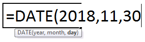
=DATE (year, month, day) where the arguments mean;

Year- It is a required argument of the function representing the number of the year of the Date. It is always expressed in four digits to avoid confusion.
Month- this is a required argument representing the number for the month of the year to use. It can be a + or – number which means the months from January (1) to December (12)
Day-it is also a required argument in Excel representing the number for the day or Date in a particular month.
It is a straightforward and more effortless function to use. Let’s get to know how to use an Excel date formula.
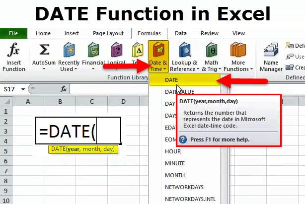
How to create and use date formula
1. Open your excel worksheet click where you need the Date created.

2. from the main menu ribbon, click on the Formulas tab.

3. Under the Function Library group, click on the drop-down arrow on the option Date& Time.

4. Select Date from the given options. Excel will display a dialog box.

5. Fill in the given fields representing the date formula.

6. Click OK. Your Date will be created and inserted into the selected cell.
Method 1: using the date formula to return a serial number for a date
For example, when you want to return a serial number that corresponds to March 14, 2021, you use the formula:
=DATE (2022, 2, 25)

But in cases where you do not want to specify the values that represent the year, month, and day directly in a formula, you can use all the arguments in other Excel date functions. You can decide to combine the YEAR and TODAY function as shown below to get a serial number:
=DATE (YEAR (TODAY ()), MONTH (TODAY ()), 14). The result will display a serial number for the fourteenth day of the current month and year.

Method 2: Using the date function to return Date based on values in other cells
When the values meant to create a date sequence are stored in different cells, all you have to do is use the date function. For example, when you have the year in cell A3, the month in cell B3, and the day in cell C3, you can use the function;
=DATE (A3, B3, C3)

Method 3: Using the date function to subtract or add dates in excel
To add or subtract some days from a given date, you first need to convert that Date into a serial number using the excel date function. For example, in the case of adding days to your date function, here is what you do;
=DATE (2022, 2, 25) + 10

When it comes to subtracting, replace the + sign with a minus sign.
Method 4: Using the date formula to convert a string of text or number to a date
The date function is beneficial when it comes to extracting Dates from a string of texts. Such scenarios occur when excel does not recognize the format used. The date function is used in liaison with other functions as stated below;
=DATE (RIGHT, MID, LEFT)

Using Date Formula to Insert Today’s Date
You can use the TODAY function to insert today’s date in any cell in Excel. The function takes no arguments but only returns today’s date. It is represented by the syntax below;
=TODAY()

The only downside is that the TODAY function is not updated automatically. Hence, if you want to update it, just press F9 or re-enter the formula. It also collects the present date from your computer; thus, it will also return a wrong date if the computer’s date is wrong.

Using Date Formula to Insert the First Day of Any Month
You can simply use 1 in place of any day argument to insert the first date of any month. It is represented by the syntax
=DATE(yy,mm,dd), where;
dd is the first day of the month, usually represented by 1.
For example; to get the first day of June of 2022, the formula will be:
=DATE(2022,6,1)

However, it becomes a challenge to extract the first date of the month from any date. For instance, assuming you want to extract the first date of the month from 21-February-2020 in cell B4, you can use the formula below;
=B4-DAY(B4)+1

If you want to extract the first date of a month from another date, you can place the date inside the date function as shown below:
=DATE(2020,5,15)-DAY(DATE(2020,5,15))+1

In this case, the DAY function returns the day number of any date inserted into it. For example, DAY(DATE(2022,5,15))+1 will return 15. Since Excel accepts any date as a numerical value, you can add or subtract dates from Excel with any number. Therefore, the above formula subtracts 15 days from the date 1st September 2022 and returns the last day of the previous month, 31-August-2022.
Using Date Formula to Insert the Last Day of Any Month
If you want to insert the last date of any month, enter the last day of that month in the day argument of the DATE function.
For example, to get the last date February 2022, the formula will be:
=DATE(2022,2,28)

However, to extract the last date of the month from any given date, you need to use the EOMONTH function, whose syntax is:
=EOMONTH(start_date,months), where;
Start_date is the last date of the month from which you want to extract the date.
Months denote the number of months you want to move forward. If you want to extract the last date of the present month, it will 0. For next month will be 1, and so on.
For example, if you want to get the last date of the month from 12-February-2022, you can use the formula below:
=EOMONTH(DATE(2022,2,12),0)

To get the last date of the month 3 months later, the formula will become:
=EOMONTH(DATE(2022,2,12),3)

Using Date Formula to Convert Date to Text
You can convert a date into text using the TEXT function of Excel with the following syntax:
=TEXT(value,format_text), where;
Value is the value you want to convert to text.
Format_text. Is the format in which you want the text to appear.
If you want to extract the names of the month of any date, you can use the formula below:
=TEXT(DATE(2022,3,20),»mmmm»)

where,
“mmmm” is the format for months.
Using Date Formula to Count Total Number of Workdays Between Two Dates
You can use the NETWORKDAYS function in excel to count the total number of work days between two days. The function is represented by the following generic formula:
=NETWORKDAYS(start_date,end_date,[holidays]), where;
Start_date is the first date.
End_date is the ending date.
[holidays] is a list of holidays.
For example; if you have a dataset with B4:B20 as a list of the holidays, you can get the total workdays between 1-January-2021 to 31-December-2022 using the following formula:
=NETWORKDAYS(DATE(2021,1,1),DATE(2022,12,31),B4:B20)

When you write the above formula in let’s say cell E4, you will get 510 as the total number of working days. However, to count the days without weekends, you use NETWORKDAYS.INTL function.
Using Date Formula to Determine the Workday After a Specific Number of Days
You can use the WORKDAY function in place of the NETWORKDAYS function to determine a specific date after a given number of workdays from a starting date. The function is represented by the syntax:
=WORKDAY(start_date,days,[holidays]), where;
Start_date is the starting date.
Days is the total number of workdays between the two dates.
[holidays] is a list of holidays.
Using the above example where you have B4:B20 as a list of holidays. You can find out the workday after 1000 days starting from 1-January-2021 using the following formula:
=WORKDAY(DATE(2021,1,1),1000,B4:B20)

Using The Date Function to Create A Series Of Dates
You can also use the DATE function to create a series of dates with specific days’ intervals. For example, if you want to create interview dates with intervals of 7 days, with 20th May 2021 as the first date, you can proceed with the following steps:
1. Enter the first date in the DATE formula. Assuming you want to use cell C4 as your first case, you can write this formula:
=DATE(2022,5,20)

2. Select all the cells in column C, go to the Home ribbon, and select Fill under the Editing list of options.

3. When you click on Fill, the drop-down menu will appear. Select Series.

4. A new Series dialogue will appear. Select Column from the Series selection, Date from the Type section, and Day from the Date Unit section.

5. Enter your interval between two dates in the Step Value. In this case, you have 7 days as your interval between two dates; hence, write 7.
6. Click OK and you see a series of interview dates displayed in the cells.

You can also use a formula to generate interview dates automatically, especially if you do not want to do it manually. In this case, the formula will be:
=DATE(2022,5,SEQUENCE(17,1,20,7))
where:
17 within the SEQUENCE function is the total number of days of the series (C4:C20).
20 is the starting date of May (20 May).
7 is the dates’ intervals.
Write the formula in cell C4 and click the Enter button. After that, you only use the Autofill Handle to drag the formula down the column to generate interview dates in the remaining cells. You can alter the formula based on your dataset. Also, remember that the SEQUENCE function is only available in Office 365.

Conclusion
From the article above, we get to know how to use Excel’s Date formula and how to create a date. The Date function has many more uses that are not mentioned above. I hope you find the information helpful.
The DATE function is a financial analyst’s best pal and categorized as a Date/Time function in Excel. The criticality of the DATE function’s role is sourced from Excel’s reluctance to keep the day, month, and year as a date. Instead, Excel stores them as a serial number.
Directly handing over dates as a text string may not work well for all Excel functions. So, we will supply the dates as a serial number using the DATE function to ensure that Excel and our worksheet formulas understand the instructions properly.

Syntax
The syntax of Excel Date function is as follows:
=DATE(year, month, day)
Arguments:
year – This is a required argument that represents the year component in the date. Enter it as a 4 digit number; entering a single digit will result in Excel automatically adding 1900 to it.
For example, entering year as ’10’ will instruct the formula to interpret the year argument as ‘1910’.
Excel refers to your computer’s date system set up to interpret the Year argument. Note that entering a negative value or a value greater than 9999 will return a #NUM! error.
month – This is a required argument that represents the month component in the date. Ideally, it must be an integer from 1 to 12 (January to December).
Alternatively, if you input a number greater than 12, Excel will count that many months starting from January of the year specified in the year argument. For example, entering year as 2001 and month as 18 will return a serial number that represents June 01, 2002. Note that Excel will return the date as the first date of the interpreted month (June 01 in our case), regardless of what you input in the date argument.
On the other hand, if you enter a value less than 1, Excel will reduce that many months from January of the year specified, plus 1. For example, if you enter month as -10 and year as 2001, Excel will return a serial number that represents February 01, 2000.
day – This is a required argument that represents the day component of the date. While in an ideal case, you will enter an integer from 1 to 31 as the date argument, it can be supplied as any other positive or negative integer and Excel will apply the same principles to compute the date as it does for the month argument.
Important characteristics of the DATE function
- DATE function returns a #NUM! error when
yearargument is supplied with a negative number or a number greater than 9999. - DATE function returns a #VALUE! error when any of its three arguments is supplied with a non-numeric value.
- If you see the Excel DATE function is returning a serial number like 36557 instead of a date, you will need to change the cell’s format. To do this, select the cell containing the returned date and search for the ‘Short Date’ option in the drop-down menu of cell formatting options in the ‘Number group’. These options sit on Excel’s Home Tab that appears at the top left.
Examples of the DATE function
Now let’s have a look at some of the examples of the DATE function in Excel.
Example 1 – The Plain – Vanilla DATE formula
In its purest form, this is what a DATE formula looks like:
=DATE(2001, 3, 15)

This formula returns a serial number that corresponds to the date March 15, 2001.
However, the formula can be slightly tweaked to incorporate the TODAY function encapsulated inside the YEAR function in Excel as well, like so:
=DATE(YEAR(TODAY()), 3, 15)

This formula will fetch the serial number for the current year (and the specified month and day), and return 03/15/2021.
Much the same way, you can use the TODAY function for the month argument as well, like so:
=DATE(YEAR(TODAY()), MONTH(TODAY()), 15)

This formula will fetch the serial number for the current year as well as the current month (and the specified day), and return 02/15/2021.
Example 2 – Using Cell References in DATE function Arguments
If the values you want to supply in the arguments are stored in cells on your spreadsheet, you can reference those cells, like so:
=DATE(A2, B2, C2)

With the values supplied from column A, the DATE function returns 04/30/2001.
Example 3 – Converting a number into a date using the DATE function
Let’s say you scalped the internet and landed on a large data set with dates written in a format that Excel does not understand (for example, 20052005).
In that (or similar) case, we can use the following formula to help Excel make sense of the data and interpret these numbers appropriately as dates:
=DATE(RIGHT(A2, 4), MID(A2, 3, 2), LEFT(A2, 2))

Recommended Reading: Excel MID Function
Addition and Subtraction of Dates With DATE function
We discussed earlier how Excel store dates as serial numbers. There is of course a logical reason why Excel does this – it enables us to add or subtract a specified number of days from a given date.
To illustrate how this works, we plugged the following formula into our sheet:
=DATE(2001, 3, 15) + 20

When you add a +20 at the end of this DATE formula, Excel will return the date 20 days after 03/15/2001, which is 04/04/2001.
Alternatively, to subtract a certain number of days, all you need to do is use a minus sign, like so:
=DATE(2001, 3, 15) - 10

But, let’s say you want to compute the number of days between today and another date. In that case, we will subtract both dates, like so:
=TODAY() - DATE(2021, 2, 20)

The formula will return the number of days between today (whenever that may be) and March 15, 2001.
Changing DATE format With DATE function
So, you added some neat formulas to your Excel sheet and everything worked out fine. But, let’s say you want to use different separators for the days (for example, ‘/’ instead of ‘-‘), or you want to use the name of the month instead of a number (for example, January instead of 01).
We discussed earlier that Excel will refer to your computer’s date format and uses the same format for displaying dates in a worksheet.
To change this format, you do not need a formula. Instead, you need to tweak some settings.
Select the cell that contains the output from the DATE function. Right-click, and choose «Format Cells». You should see the following dialogue box:

Choose the format of your preference and click «OK».
Conditional Formatting with DATE function
Let’s say you have a large data set and you want to separate the data points occurring before and after a certain date.
To do this, we will use Excel’s conditional formatting rules and instruct Excel to shade these 2 cells with 2 separate colors so it becomes easy for us to discern.
We have our dates listed out in column A, and we want to shade the dates occurring before 12/31/2012 in green, and the ones occurring after in red.
To illustrate the entire process, we will use the following formula as a starting point:
=$A2 < DATE(2012, 12, 31)

Notice how this formula returns a Boolean value but does not shade any cells.
Let’s move a step further and apply a shade.
Select the range A2:A8 and navigate to the «Conditional Formatting» drop-down menu in the «Styles» group under the «Home» tab, and select «Manage Rules»:

On the «Conditional Formatting Rules Manager» click the «New Rule» button.

After clicking on the «New Rule» you will see a list of Rule Types. Scroll over to «Use a formula to determine which cells to format» and choosing it will reveal a formula box. In this box, plug in the formula we used to fetch Boolean values and select the desired formatting, like so:

Click «OK» and you should return to the Conditional Formatting Rules Manager dialog box.
To shade the dates occurring after 12/21/2012 red, we will add another rule following the same process. The only difference, obviously, will be in the formula. Instead of using a ‘<‘, we will use a ‘>=’, like so: =$A2>=DATE(2012,12,31)

This is what the Rules Manager box should look like at this point. Make sure that the «Applies to» box contains the appropriate range.

As your final step, click on «Apply» and watch your date list switch colors.

I hope the guide gives you a confidence boost the next time you use DATE formulas in your worksheet. Remember, practice is key. By the time you are done practicing, we will have another Excel function for you to explore.
DATE in Excel (Table of Contents)
- DATE in Excel
- DATE Formula in Excel
- How to Use DATE Function in Excel?
Introduction to Excel DATE Function
The date function is quite helpful for creating the dates that consider Month, Year, and Day. We can feed any number here, and the Date function will create the date with respect to the value we feed in. This function is quite useful and helpful for structuring the date standards when we have multiple dates in multiple formats, and we want to standardize this with a single type for all.
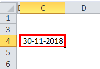
Let us look at the below simple examples. First, enter the number 43434 in excel and give the format as DD-MM-YYY.
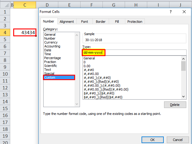
Once the above format is given, now look at how excel shows up that number.
Now give the format as [hh]:mm: ss, and the display will be as per the below image.
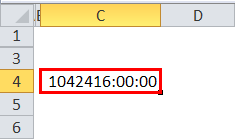
So excel completely works on numbers and their formats.
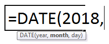
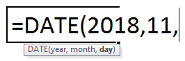
By using the DATE Function in Excel, we can create an accurate date. For example, =DATE (2018, 11, 14) would give the result as 14-11-2018.
DATE Formula in Excel
The Formula for the DATE Function in Excel is as follows:
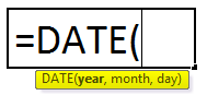
The Formula of DATE function includes 3 arguments, i.e. Year, Month, and Day.
1. Year: It is the mandatory parameter. A year is always a 4-digit number; since it is a number, we need not to specify the number in any double-quotes.
2. Month: This is also a mandatory parameter. A month should be a 2-digit number that can be supplied either directly to the cell reference or direct supply to the parameter.
3. Day: It is also a mandatory parameter. A day should be a 2-digit number.
How to Use DATE Function in Excel?
This DATE Function in Excel is very simple easy to use. Let us now see how to use the DATE Function in Excel with the help of some examples.
You can download this DATE Function Excel Template here – DATE Function Excel Template
Example #1
From the below data, create full date values. In the first column, we have days; in the second column, we have a month; and in the third column, we have a year. We need to combine these three columns and create a full date.
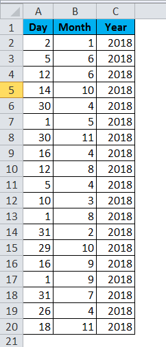
Enter the above into an excel sheet and apply the below formula to get the full date value.
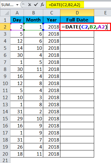
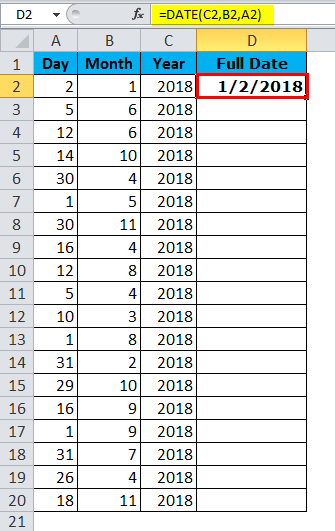
The Full DATE value is given below:
Example #2
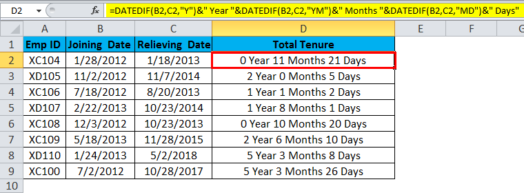
Find the difference between two days in terms of Total Years, Total Month, and Days. For example, assume you are working in an HR department in a company, and you have employee joining date and relieving date data. Next, you need to find the total tenure in the company. For example, 4 Years, 5 Months, 12 Days.
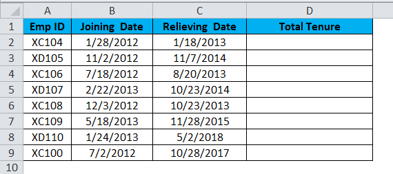
Here we need to use the DATEDIF function to get the result as per our wish. DATE function alone cannot do the job for us. If we just deduct the relieving date with the joining date, we get the only number of days they worked; we get in detail.
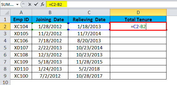
In order to get the full result, i.e. Total Tenure, we need to use the DATEDIF function.
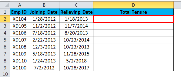
DATEDIF function is an undocumented formula where there is no IntelliSense list for it. This can be useful to find the difference between year, month, and day.
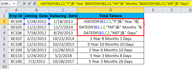
The formula looks like a lengthy one. However, I will break it down in detail.
Part 1: =DATEDIF (B2,C2, “Y”) this is the starting date and ending date, and “Y” means we need to know the difference between years.
Part 2: &” Year” This part is just added to a previous part of the foSo, forla. For example, if the first part gives, 4 then the result will be 4 Years.
Part 3: &DATEDIF(B2, C2, “YM”) Now, we found the difference between years. In this part of the formula, we are finding the difference between the months. “YM” can give the difference between months.
Part 4: &” Months” This is the addition to part 3. If the result of part 3 is 4, then this part will add Months to part 3, i.e. 3 Months
Part 5: “&DATEDIF(B2, C2,” MD”) now we have a difference between Year and the Month. In this part, we are finding the difference between the days. “MD” can give us that difference.
Part 6: &” Days” is added into part 5. If the result from part 5 is 25, then it will add Days to it. I.e. 25 Days.
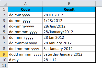
Example #3
Now I will explain to you the different date formats in excel. There are many date formats in excel each show up the result differently.
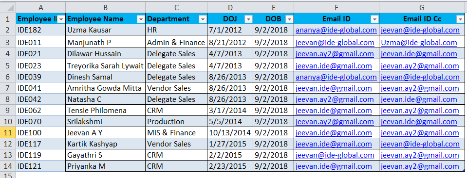
VBA Example with Date in Excel:
Assume you are in the welfare team of the company, and you need to send birthday emails to your employees if there are any birthdays. However, sending each one of them is a tedious task. So here, I have developed a code to auto-send birthday wishes.
Below is the list of employees and their birthdays.
I have already written a code to send the birthday emails to everyone if there is any birthday today.
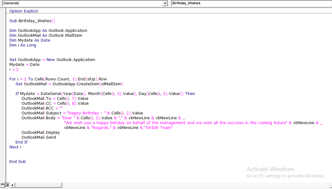
Write the above in your VBA module and save the workbook as a macro-enabled workbook.
Once the above code is written on the VBA module, save the workbook.
The only thing you need to do is add your data to the excel sheet and run the code every day you come to an office.
Things to Remember
- The given number should be >0 and <10000; otherwise, excel will give the error as #NUM!
- We can supply only numerical values. Anything other than numerical values, we will get eh error as #VALUE!
- Excel stores date as serial numbers and show the display according to the format.
- Always enter a full-year value. Do not enter any shortcut years like 18, 19, and 20, etc. Instead, enter the full year 2017, 2018, 2020
Recommended Articles
This is a guide to Excel DATE Function. Here we discuss the DATE Formula in Excel and how to use the DATE Function in Excel along with excel examples and downloadable excel templates. You may also look at these useful functions in excel –
- EDATE Excel Function
- Compare Dates in Excel
- Subtract Date In Excel
- VBA Date
The DATE function creates a date using individual year, month, and day arguments. Each argument is provided as a number, and the result is a serial number that represents a valid Excel date. Apply a date number format to display the output from the DATE function as a date.
In general, the DATE function is the safest way to create a date in an Excel formula, because year, month, and day values are numeric and unambiguous, in contrast to text representations of dates which can be misinterpreted.
Note: to move an existing date forward or backward in time, see the EDATE and EOMONTH.
Example #1 — hard-coded numbers
For example, you can use the DATE function to create the dates January 1, 1999, and June 1, 2010 with the following syntax:
=DATE(1999,1,1) // returns Jan 1, 1999
=DATE(2010,6,1) // returns Jun 1, 2010
Example #2 — cell reference
The DATE function is useful for assembling dates that need to change dynamically based on other inputs in a worksheet. For example, with 2018 in cell A1, the formula below returns the date April 15, 2018:
=DATE(A1,4,15) // Apr 15, 2018
If A1 is then changed to 2019, the DATE function will return a date for April 15, 2019.
Example #3 — with SUMIFS, COUNTIFS
The DATE function can be used to supply dates as inputs to other functions like SUMIFS or COUNTIFS, since you can easily assemble a date using year, month, and day values that come from a cell reference or formula result. For example, to count dates greater than January 1, 2019 in a worksheet where A1, B1, and C1 contain year, month, and day values (respectively), you can use a formula like this:
=COUNTIF(range,">"&DATE(A1,B1,C1))
The result of COUNTIF will update dynamically when A1, B1, or C1 are changed.
Example #4 — first day of current year
To return the first day of the current year, you can use the DATE function like this:
=DATE(YEAR(TODAY()),1,1) // first of year
This is an example of nesting. The TODAY function returns the current date to the YEAR function. The YEAR function extracts the year and returns the result to the DATE function as the year argument. The month and day arguments are hard-coded as 1. The result is the first day of the current year, a date like «January 1, 2021».
Note: the DATE function actually returns a serial number and not a formatted date. In Excel’s date system, dates are serial numbers. January 1, 1900 is number 1 and later dates are larger numbers. To display date values in a human-readable date format, apply the number format of your choice.
Notes
- The DATE function returns a serial number that corresponds to an Excel date.
- Excel dates begin in the year 1900. If year is between zero and 1900, Excel will add 1900.
- The DATE function accepts numeric input only and will return #VALUE if given text.