
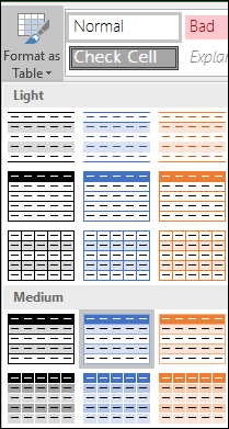
Excel provides numerous predefined table styles that you can use to quickly format a table. If the predefined table styles don’t meet your needs, you can create and apply a custom table style. Although you can delete only custom table styles, you can remove any predefined table style so that it is no longer applied to a table.

You can further adjust the table formatting by choosing Quick Styles options for table elements, such as Header and Total Rows, First and Last Columns, Banded Rows and Columns, as well as Auto Filtering.
Note: The screen shots in this article were taken in Excel 2016. If you have a different version your view might be slightly different, but unless otherwise noted, the functionality is the same.
Choose a table style
When you have a data range that is not formatted as a table, Excel will automatically convert it to a table when you select a table style. You can also change the format for an existing table by selecting a different format.
-
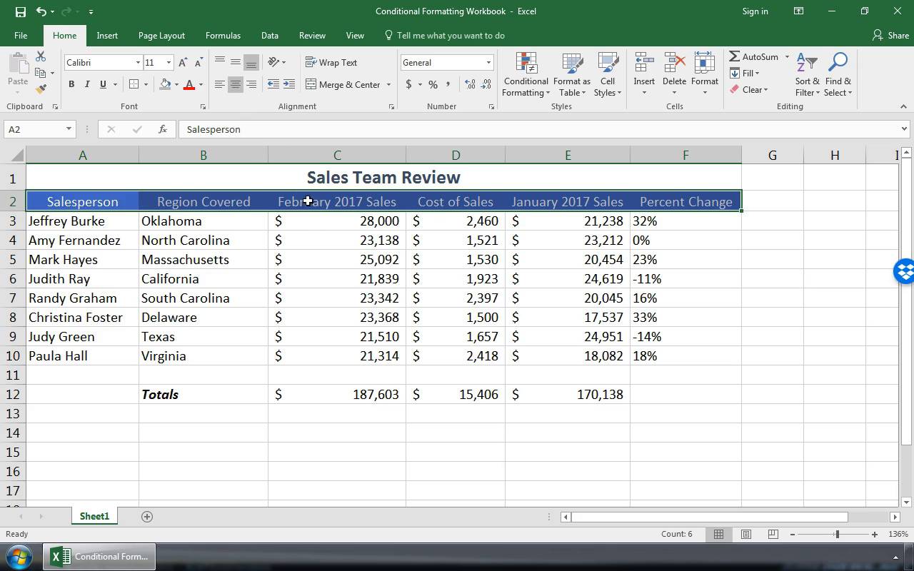
Select any cell within the table, or range of cells you want to format as a table.
-
On the Home tab, click Format as Table.

-
Click the table style that you want to use.
Notes:
-
Auto Preview — Excel will automatically format your data range or table with a preview of any style you select, but will only apply that style if you press Enter or click with the mouse to confirm it. You can scroll through the table formats with the mouse or your keyboard’s arrow keys.
-
When you use Format as Table, Excel automatically converts your data range to a table. If you don’t want to work with your data in a table, you can convert the table back to a regular range while keeping the table style formatting that you applied. For more information, see Convert an Excel table to a range of data.
Important:
-
Once created, custom table styles are available from the Table Styles gallery under the Custom section.
-
Custom table styles are only stored in the current workbook, and are not available in other workbooks.
Create a custom table style
-
Select any cell in the table you want to use to create a custom style.
-
On the Home tab, click Format as Table, or expand the Table Styles gallery from the Table Tools > Design tab (the Table tab on a Mac).
-
Click New Table Style, which will launch the New Table Style dialog.
-
In the Name box, type a name for the new table style.
-
In the Table Element box, do one of the following:
-
To format an element, click the element, then click Format, and then select the formatting options you want from the Font, Border or Fill tabs.
-
To remove existing formatting from an element, click the element, and then click Clear.
-
-
Under Preview, you can see how the formatting changes that you made affect the table.
-
To use the new table style as the default table style in the current workbook, select the Set as default table style for this document check box.

Delete a custom table style
-
Select any cell in the table from which you want to delete the custom table style.
-
On the Home tab, click Format as Table, or expand the Table Styles gallery from the Table Tools > Design tab (the Table tab on a Mac).
-
Under Custom, right-click the table style that you want to delete, and then click Delete on the shortcut menu.
Note: All tables in the current workbook that are using that table style will be displayed in the default table format.
-
Select any cell in the table from which you want to remove the current table style.
-
On the Home tab, click Format as Table, or expand the Table Styles gallery from the Table Tools > Design tab (the Table tab on a Mac).
-
Click Clear.
The table will be displayed in the default table format.
Note: Removing a table style does not remove the table. If you don’t want to work with your data in a table, you can convert the table to a regular range. For more information, see Convert an Excel table to a range of data.
There are several table style options that can be toggled on and off. To apply any of these options:
-
Select any cell in the table.
-
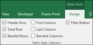
Go to Table Tools > Design, or the Table tab on a Mac, and in the Table Style Options group, check or uncheck any of the following:
-
Header Row — Apply or remove formatting from the first row in the table.
-
Total Row — Quickly add SUBTOTAL functions like SUM, AVERAGE, COUNT, MIN/MAX to your table from a drop-down selection. SUBTOTAL functions allow you to include or ignore hidden rows in calculations.
-
First Column — Apply or remove formatting from the first column in the table.
-
Last Column — Apply or remove formatting from the last column in the table.
-
Banded Rows — Display odd and even rows with alternating shading for ease of reading.
-
Banded Columns — Display odd and even columns with alternating shading for ease of reading.
-
Filter Button — Toggle AutoFilter on and off.
-
In Excel for the web, you can apply table style options to format the table elements.
Choose table style options to format the table elements
There are several table style options that can be toggled on and off. To apply any of these options:
-
Select any cell in the table.
-
On the Table Design tab, under Style Options, check or uncheck any of the following:
-
Header Row — Apply or remove formatting from the first row in the table.
-
Total Row — Quickly add SUBTOTAL functions like SUM, AVERAGE, COUNT, MIN/MAX to your table from a drop-down selection. SUBTOTAL functions allow you to include or ignore hidden rows in calculations.
-
Banded Rows — Display odd and even rows with alternating shading for ease of reading.
-
First Column — Apply or remove formatting from the first column in the table.
-
Last Column — Apply or remove formatting from the last column in the table.
-
Banded Columns — Display odd and even columns with alternating shading for ease of reading.
-
Filter Button — Toggle AutoFilter on and off.
-
Create and format tables
Create and format a table to visually group and analyze data.
Note: Excel tables shouldn’t be confused with the data tables that are part of a suite of What-If Analysis commands (Forecast, on the Data tab). See Introduction to What-If Analysis for more information.

Try it!
-
Select a cell within your data.
-
Select Home > Format as Table.
-
Choose a style for your table.
-
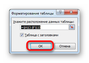
In the Create Table dialog box, set your cell range.
-
Mark if your table has headers.
-
Select OK.
-
Insert a table in your spreadsheet. See Overview of Excel tables for more information.
-
Select a cell within your data.
-
Select Home > Format as Table.
-
Choose a style for your table.
-
In the Create Table dialog box, set your cell range.
-
Mark if your table has headers.
-
Select OK.
To add a blank table, select the cells you want included in the table and click Insert > Table.
To format existing data as a table by using the default table style, do this:
-
Select the cells containing the data.
-
Click Home > Table > Format as Table.
-
If you don’t check the My table has headers box, Excel for the web adds headers with default names like Column1 and Column2 above the data. To rename a default header, double-click it and type a new name.
Note: You can’t change the default table formatting in Excel for the web.
Want more?
Overview of Excel tables
Video: Create and format an Excel table
Total the data in an Excel table
Format an Excel table
Resize a table by adding or removing rows and columns
Filter data in a range or table
Convert a table to a range
Using structured references with Excel tables
Excel table compatibility issues
Export an Excel table to SharePoint
Need more help?
Содержание
- Форматирование таблиц
- Автоформатирование
- Переход к форматированию
- Форматирование данных
- Выравнивание
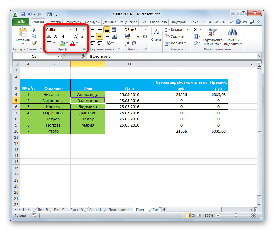
- Шрифт
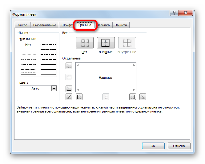
- Граница
- Заливка
- Защита
- Вопросы и ответы

Одним из самых важных процессов при работе в программе Excel является форматирование. С его помощью не только оформляется внешний вид таблицы, но и задается указание того, как программе воспринимать данные, расположенные в конкретной ячейке или диапазоне. Без понимания принципов работы данного инструмента нельзя хорошо освоить эту программу. Давайте подробно выясним, что же представляет собой форматирование в Экселе и как им следует пользоваться.
Урок: Как форматировать таблицы в Microsoft Word
Форматирование таблиц
Форматирование – это целый комплекс мер регулировки визуального содержимого таблиц и расчетных данных. В данную область входит изменение огромного количества параметров: размер, тип и цвет шрифта, величина ячеек, заливка, границы, формат данных, выравнивание и много другое. Подробнее об этих свойствах мы поговорим ниже.
Автоформатирование
К любому диапазону листа с данными можно применить автоматическое форматирование. Программа отформатирует указанную область как таблицу и присвоит ему ряд предустановленных свойств.
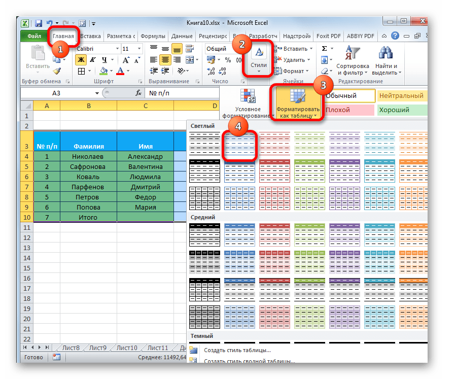
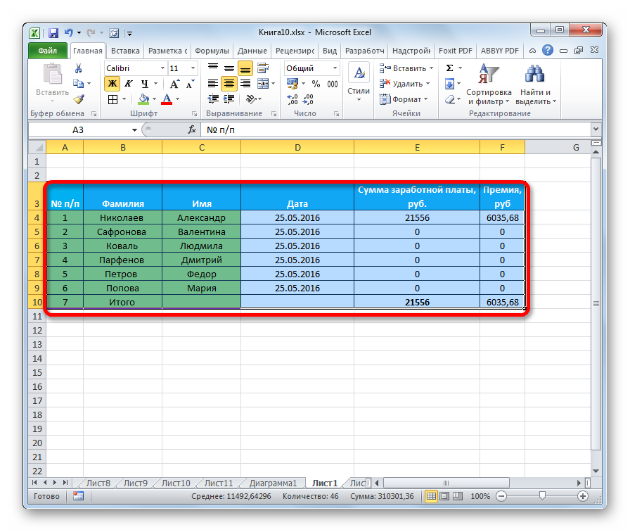
- Выделяем диапазон ячеек или таблицу.
- Находясь во вкладке «Главная» кликаем по кнопке «Форматировать как таблицу». Данная кнопка размещена на ленте в блоке инструментов «Стили». После этого открывается большой список стилей с предустановленными свойствами, которые пользователь может выбрать на свое усмотрение. Достаточно просто кликнуть по подходящему варианту.
- Затем открывается небольшое окно, в котором нужно подтвердить правильность введенных координат диапазона. Если вы выявили, что они введены не верно, то тут же можно произвести изменения. Очень важно обратить внимание на параметр «Таблица с заголовками». Если в вашей таблице есть заголовки (а в подавляющем большинстве случаев так и есть), то напротив этого параметра должна стоять галочка. В обратном случае её нужно убрать. Когда все настройки завершены, жмем на кнопку «OK».

После этого, таблица будет иметь выбранный формат. Но его можно всегда отредактировать с помощью более точных инструментов форматирования.
Переход к форматированию
Пользователей не во всех случаях удовлетворяет тот набор характеристик, который представлен в автоформатировании. В этом случае, есть возможность отформатировать таблицу вручную с помощью специальных инструментов.
Перейти к форматированию таблиц, то есть, к изменению их внешнего вида, можно через контекстное меню или выполнив действия с помощью инструментов на ленте.
Для того, чтобы перейти к возможности форматирования через контекстное меню, нужно выполнить следующие действия.
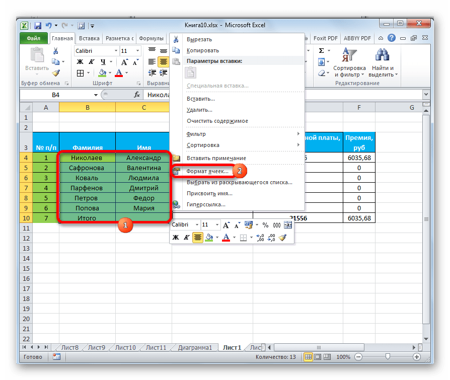
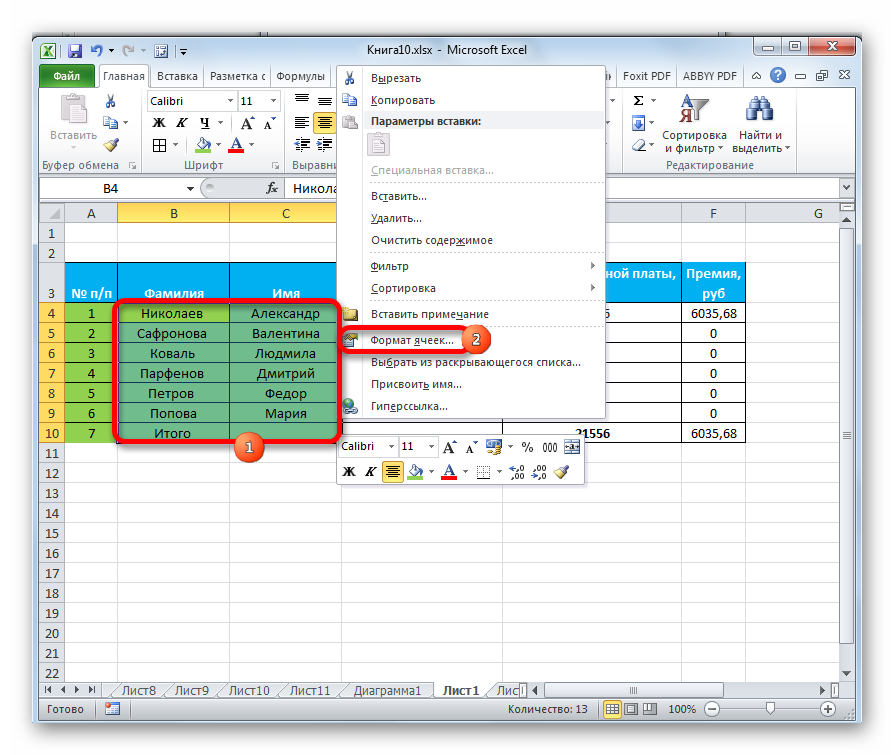
- Выделяем ячейку или диапазон таблицы, который хотим отформатировать. Кликаем по нему правой кнопкой мыши. Открывается контекстное меню. Выбираем в нем пункт «Формат ячеек…».
- После этого открывается окно формата ячеек, где можно производить различные виды форматирования.

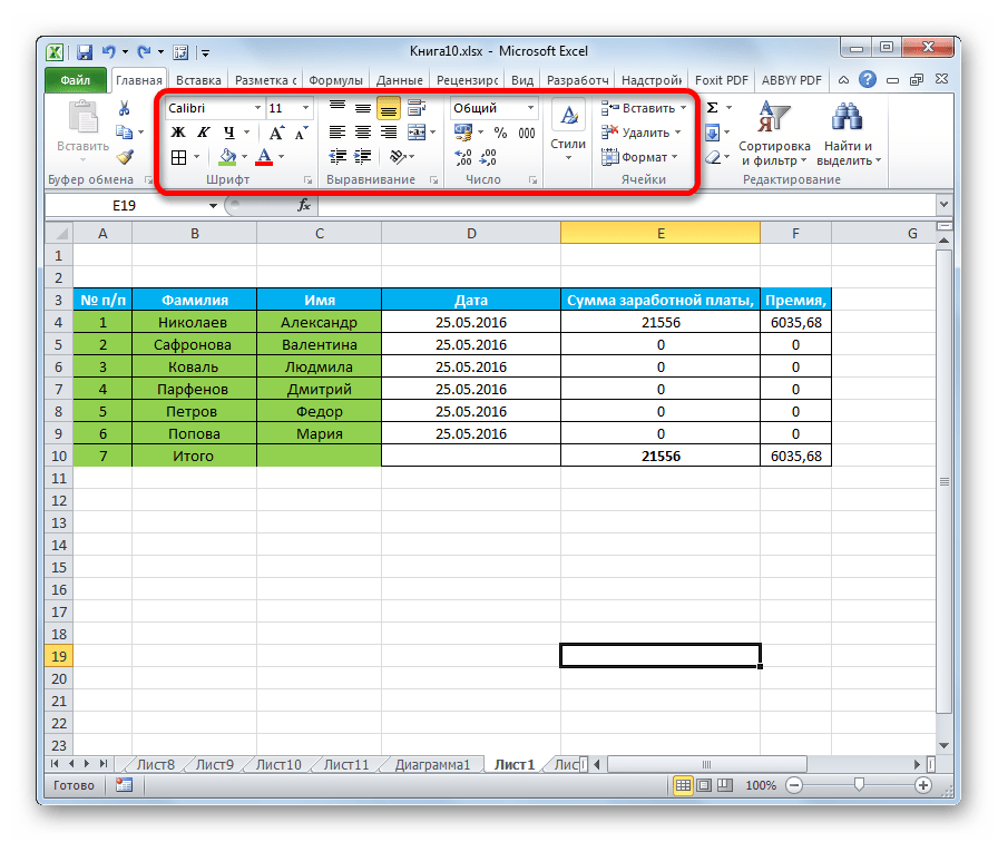
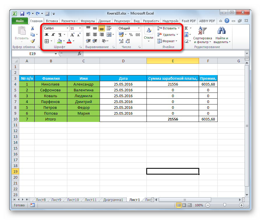
Инструменты форматирования на ленте находятся в различных вкладках, но больше всего их во вкладке «Главная». Для того, чтобы ими воспользоваться, нужно выделить соответствующий элемент на листе, а затем нажать на кнопку инструмента на ленте.
Форматирование данных
Одним из самых важных видов форматирования является формат типа данных. Это обусловлено тем, что он определяет не столько внешний вид отображаемой информации, сколько указывает программе, как её обрабатывать. Эксель совсем по разному производит обработку числовых, текстовых, денежных значений, форматов даты и времени. Отформатировать тип данных выделенного диапазона можно как через контекстное меню, так и с помощью инструмента на ленте.
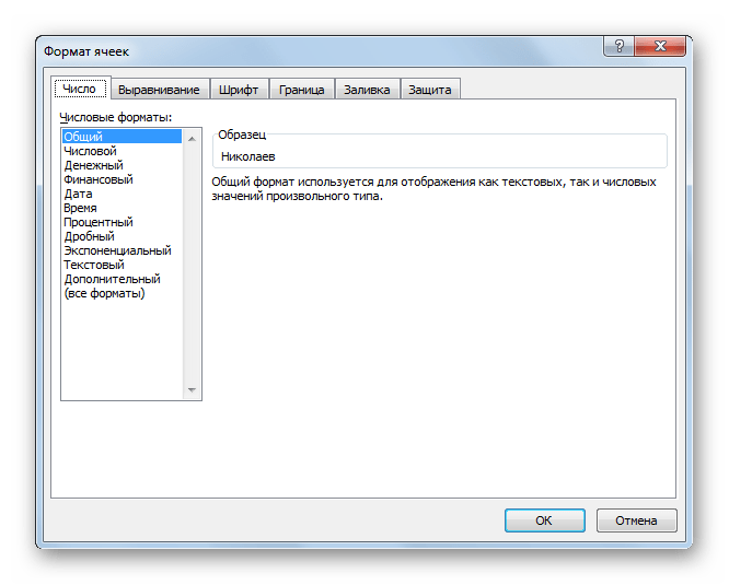
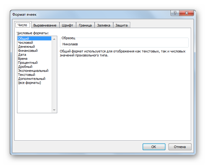
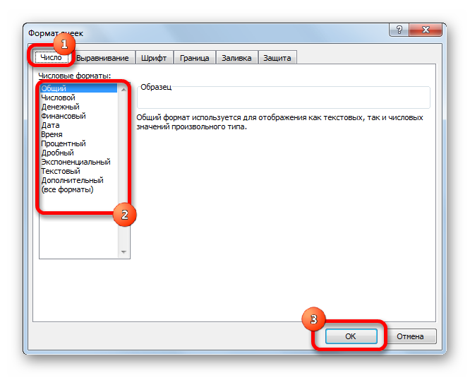
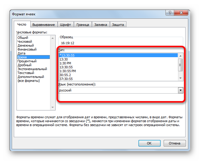
Если вы откроете окно «Формат ячеек» чрез контекстное меню, то нужные настройки будут располагаться во вкладке «Число» в блоке параметров «Числовые форматы». Собственно, это единственный блок в данной вкладке. Тут производится выбор одного из форматов данных:
- Числовой;
- Текстовый;
- Время;
- Дата;
- Денежный;
- Общий и т.д.
После того, как выбор произведен, нужно нажать на кнопку «OK».

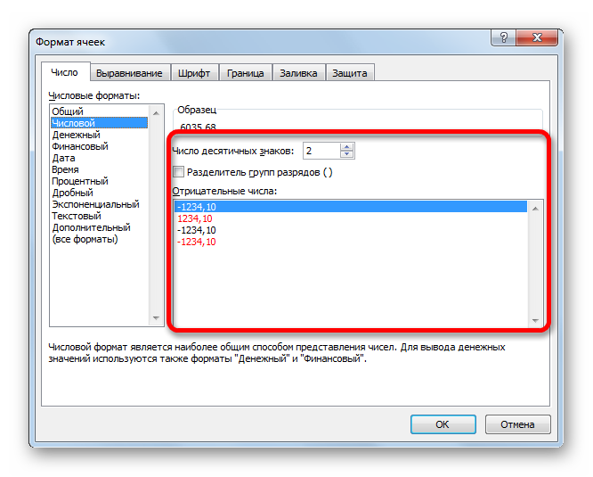
Кроме того, для некоторых параметров доступны дополнительные настройки. Например, для числового формата в правой части окна можно установить, сколько знаков после запятой будет отображаться у дробных чисел и показывать ли разделитель между разрядами в числах.

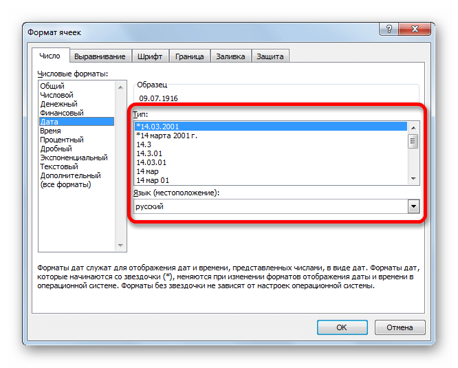
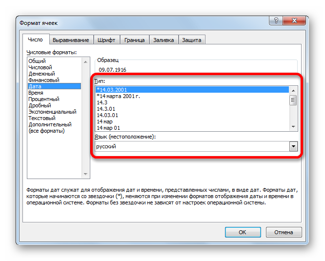
Для параметра «Дата» доступна возможность установить, в каком виде дата будет выводиться на экран (только числами, числами и наименованиями месяцев и т.д.).
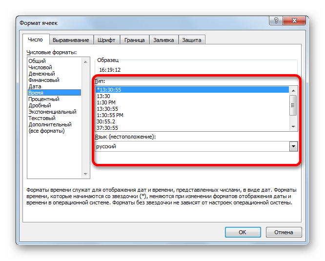
Аналогичные настройки имеются и у формата «Время».
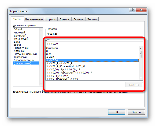
Если выбрать пункт «Все форматы», то в одном списке будут показаны все доступные подтипы форматирования данных.
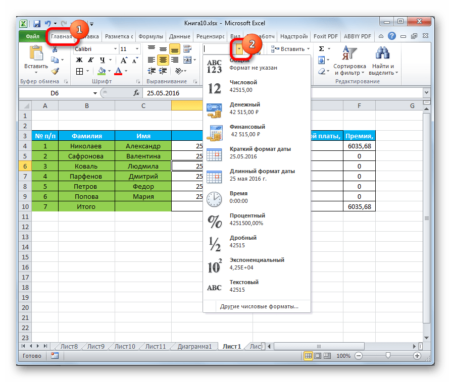
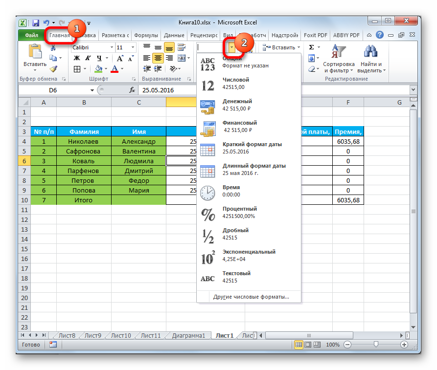
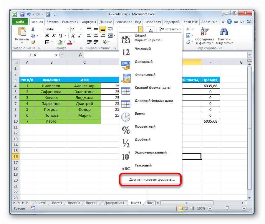
Если вы хотите отформатировать данные через ленту, то находясь во вкладке «Главная», нужно кликнуть по выпадающему списку, расположенному в блоке инструментов «Число». После этого раскрывается перечень основных форматов. Правда, он все-таки менее подробный, чем в ранее описанном варианте.
Впрочем, если вы хотите более точно произвести форматирование, то в этом списке нужно кликнуть по пункту «Другие числовые форматы…». Откроется уже знакомое нам окно «Формат ячеек» с полным перечнем изменения настроек.

Урок: Как изменить формат ячейки в Excel
Выравнивание
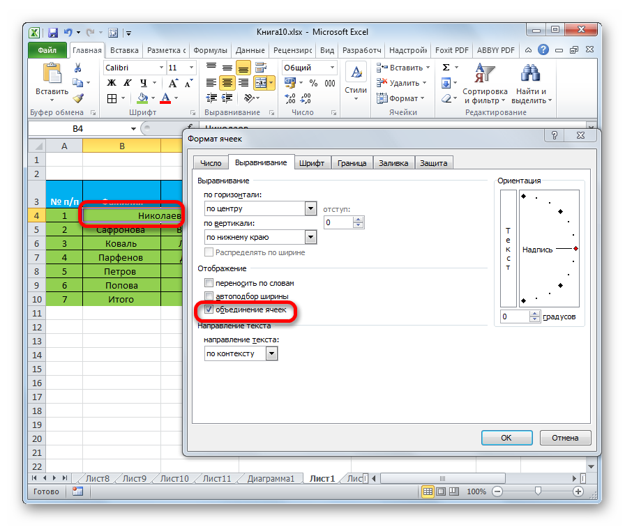
Целый блок инструментов представлен во вкладке «Выравнивание» в окне «Формат ячеек».
Путем установки птички около соответствующего параметра можно объединять выделенные ячейки, производить автоподбор ширины и переносить текст по словам, если он не вмещается в границы ячейки.

Кроме того, в этой же вкладке можно позиционировать текст внутри ячейки по горизонтали и вертикали.
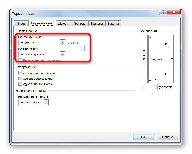
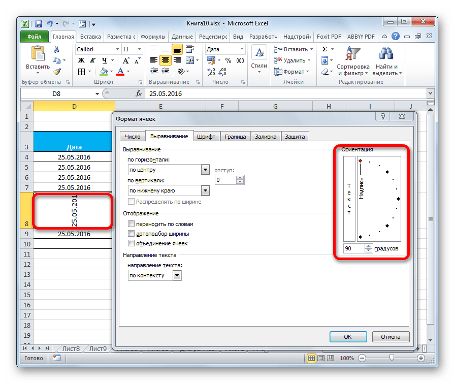
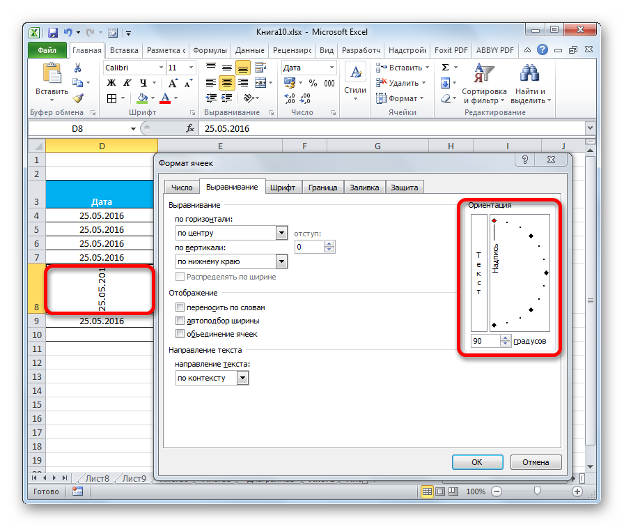
В параметре «Ориентация» производится настройка угла расположения текста в ячейке таблицы.
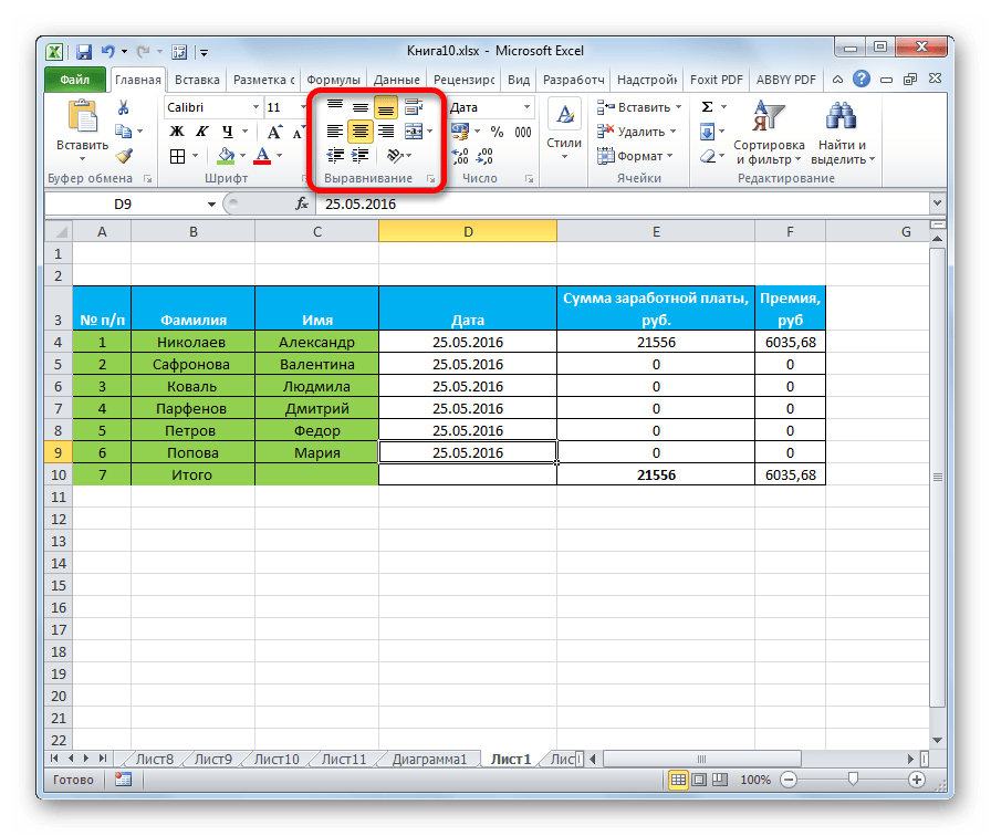
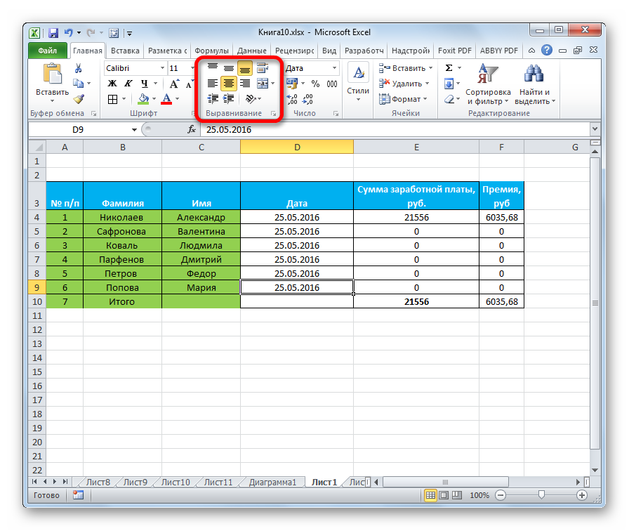
Блок инструментов «Выравнивание» имеется так же на ленте во вкладке «Главная». Там представлены все те же возможности, что и в окне «Формат ячеек», но в более усеченном варианте.
Шрифт
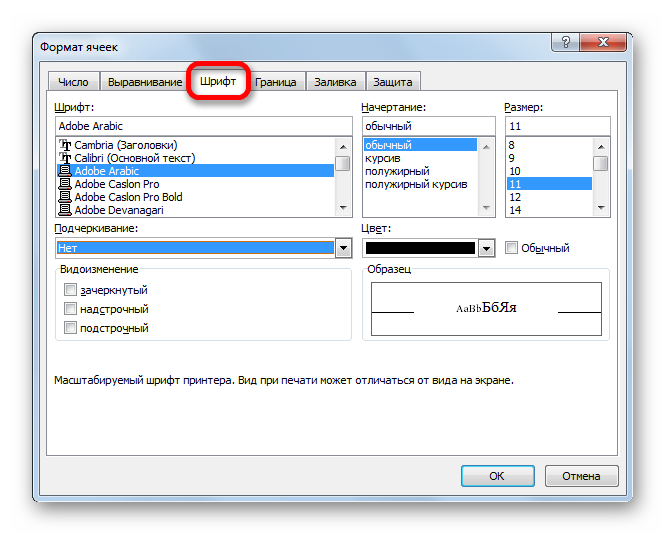
Во вкладке «Шрифт» окна форматирования имеются широкие возможности по настройке шрифта выделенного диапазона. К этим возможностям относятся изменение следующих параметров:
- тип шрифта;
- начертание (курсив, полужирный, обычный)
- размер;
- цвет;
- видоизменение (подстрочный, надстрочный, зачеркнутый).

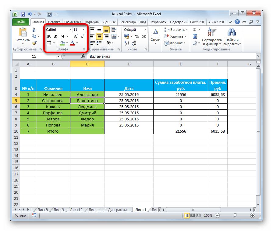
На ленте тоже имеется блок инструментов с аналогичными возможностями, который также называется «Шрифт».
Граница
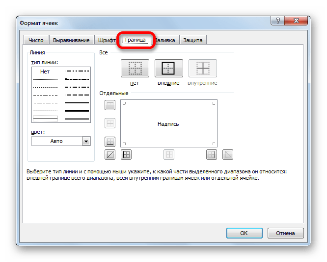
Во вкладке «Граница» окна форматирования можно настроить тип линии и её цвет. Тут же определяется, какой граница будет: внутренней или внешней. Можно вообще убрать границу, даже если она уже имеется в таблице.
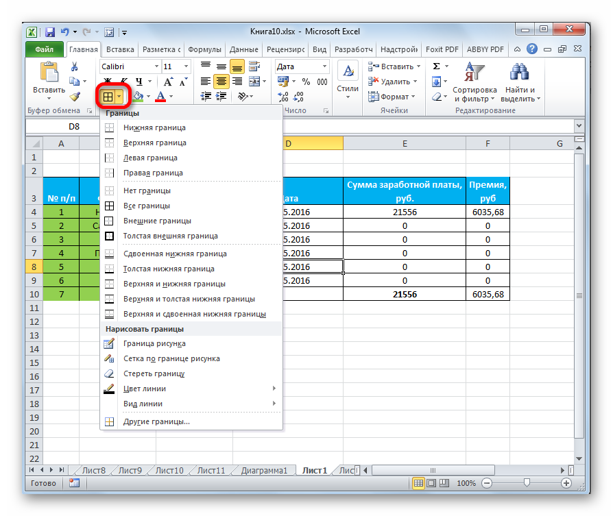
А вот на ленте нет отдельного блока инструментов для настроек границы. Для этих целей во вкладке «Главная» выделена только одна кнопка, которая располагается в группе инструментов «Шрифт».
Заливка
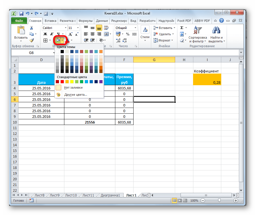
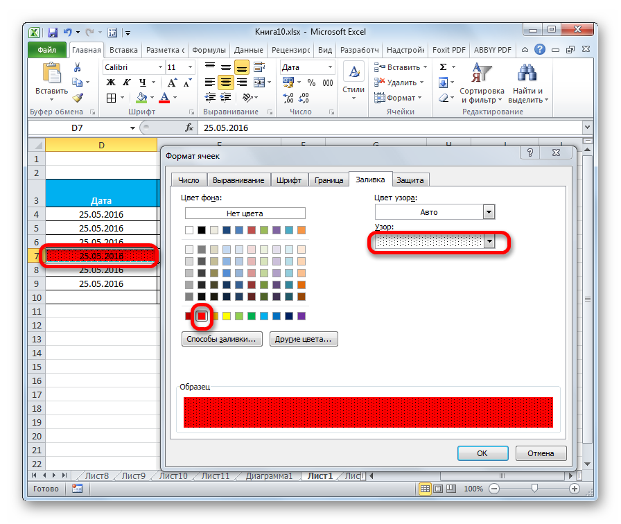
Во вкладке «Заливка» окна форматирования можно производить настройку цвета ячеек таблицы. Дополнительно можно устанавливать узоры.

На ленте, как и для предыдущей функции для заливки выделена всего одна кнопка. Она также размещается в блоке инструментов «Шрифт».
Если представленных стандартных цветов вам не хватает и вы хотите добавить оригинальности в окраску таблицы, тогда следует перейти по пункту «Другие цвета…».
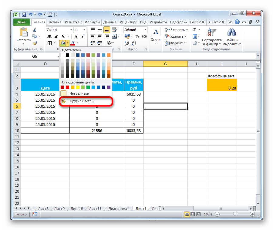
После этого открывается окно, предназначенное для более точного подбора цветов и оттенков.

Защита
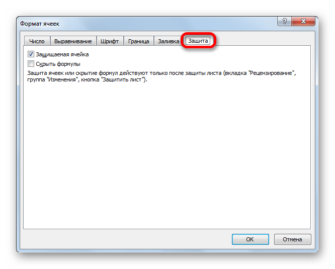
В Экселе даже защита относится к области форматирования. В окне «Формат ячеек» имеется вкладка с одноименным названием. В ней можно обозначить, будет ли защищаться от изменений выделенный диапазон или нет, в случае установки блокировки листа. Тут же можно включить скрытие формул.
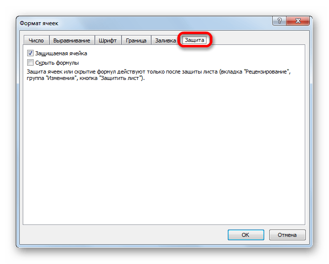
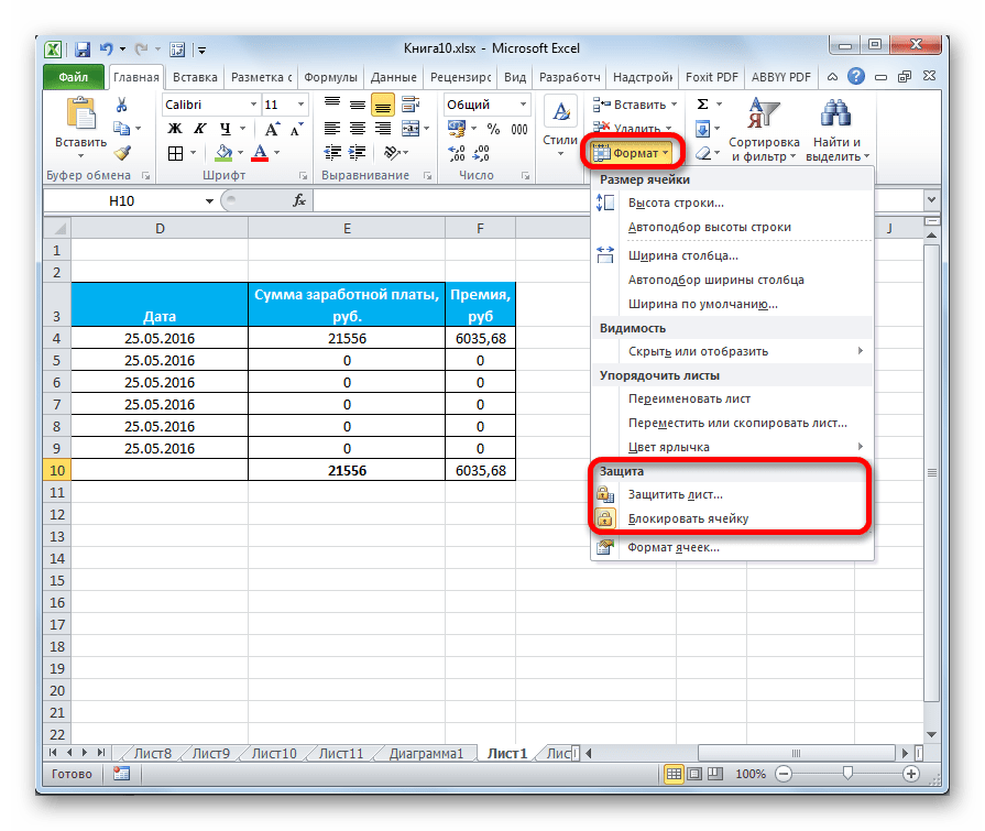
На ленте аналогичные функции можно увидеть после клика по кнопке «Формат», которая расположена во вкладке «Главная» в блоке инструментов «Ячейки». Как видим, появляется список, в котором имеется группа настроек «Защита». Причем тут можно не только настроить поведение ячейки в случае блокировки, как это было в окне форматирования, но и сразу заблокировать лист, кликнув по пункту «Защитить лист…». Так что это один из тех редких случаев, когда группа настроек форматирования на ленте имеет более обширный функционал, чем аналогичная вкладка в окне «Формат ячеек».
.
Урок: Как защитить ячейку от изменений в Excel
Как видим, программа Excel обладает очень широким функционалом по форматированию таблиц. При этом, можно воспользоваться несколькими вариантами стилей с предустановленными свойствами. Также можно произвести более точные настройки при помощи целого набора инструментов в окне «Формат ячеек» и на ленте. За редким исключением в окне форматирования представлены более широкие возможности изменения формата, чем на ленте.
Во время работы в Эксель, наряду с добавлением и обработкой данных, очень важно наилучшим образом представить информацию (цвет, размер, тип шрифта, границы, заливка, выравнивание и т.д.), чтобы она была максимально информативной и легко воспринимаемой. В этом поможет форматирование таблицы, с помощью которого, помимо прочего, можно задать тип данных, чтобы программа могла правильно идентифицировать те или иные разновидности значений в ячейках. В данной статье мы рассмотрим, каким образом выполняется форматирование в Excel.
- Трансформация в “Умную таблицу”
-
Ручное форматирование
- Выбор типа данных
- Выравнивание содержимого
- Настройка шрифта
-
Границы и линии
- Заливка ячеек
- Защита данных
- Заключение
Трансформация в “Умную таблицу”
Выбрав определенную область данных в таблице, можно воспользоваться такой опцией как автоформатирование. Эксель автоматически выполнить преобразование выделенного диапазона в таблицу. Вот как это делается:
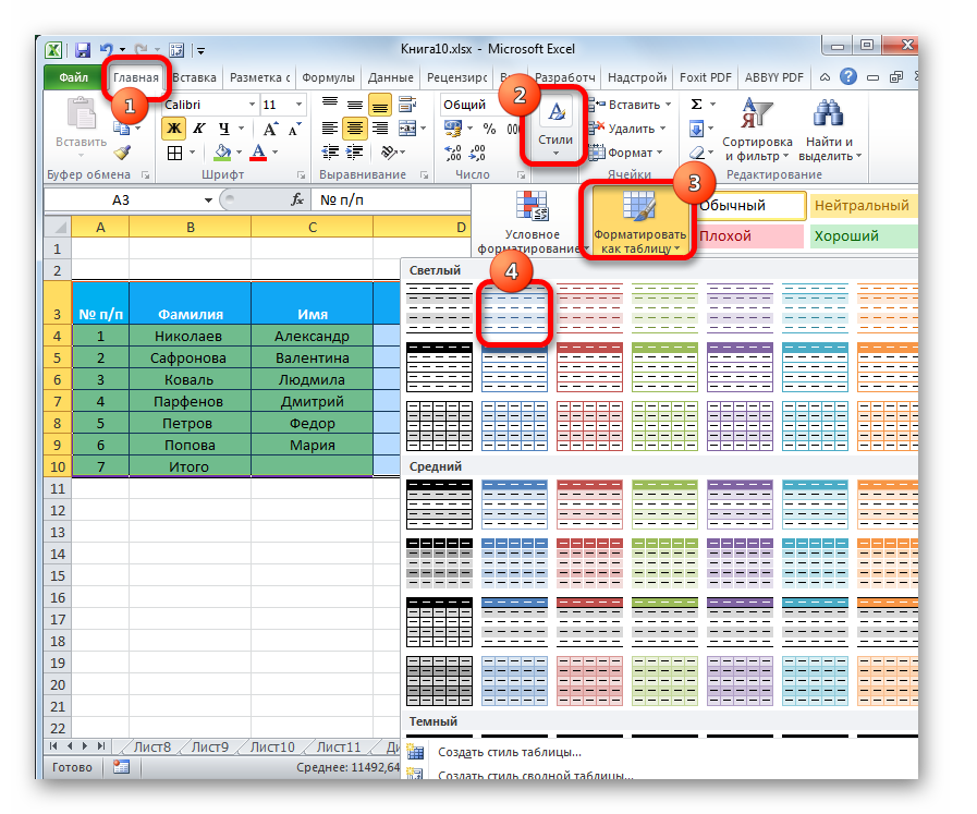
- Производим выделение нужных элементов. На ленте программы находим группу инструментов “Стили” (вкладка “Главная“) и жмем кнопку “Форматировать как таблицу”.

- Раскроется перечень различных стилей с заранее выполненными настройками. Мы можем выбрать любой из них, кликнув по понравившемуся варианту.

- На экране появится вспомогательное окошко, где будут отображаться координаты выделенного в первом шаге диапазона. В случае необходимости адреса ячеек можно скорректировать (вручную или выделив заново требуемую область в самой таблице). При наличии шапки таблицы в выделении обязательно ставим напротив пункта “Таблица с заголовками” галочку. Далее щелкаем OK.

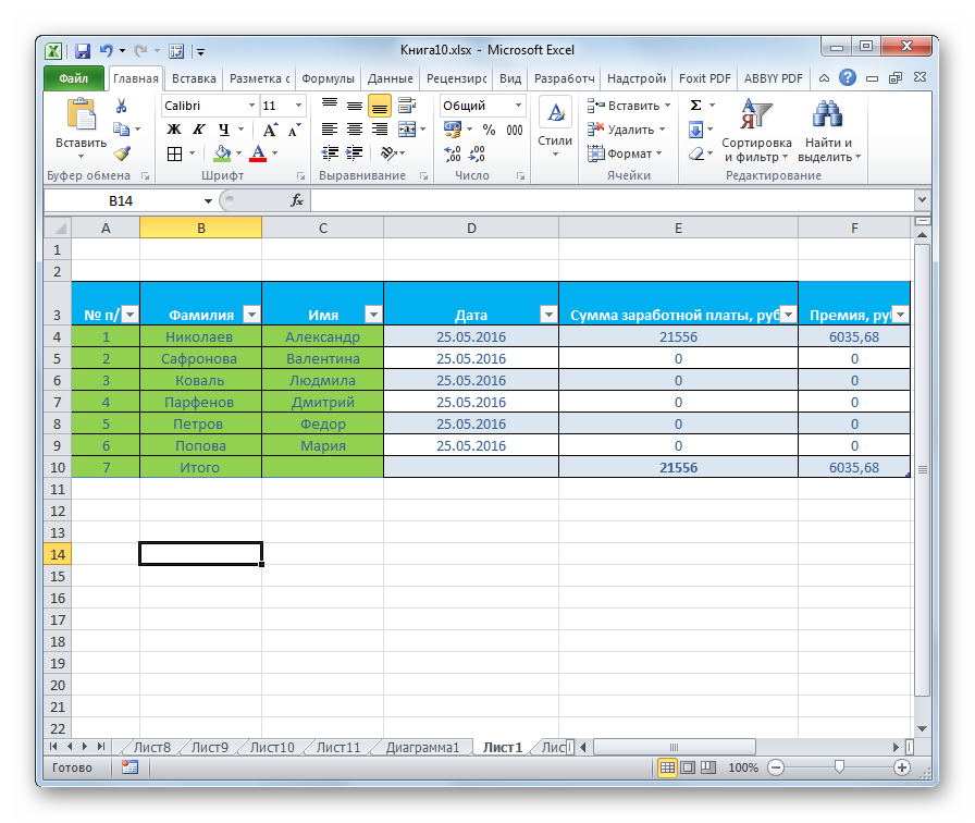
- В результате, наша таблица трансформируется в так называемую “умную таблицу”.


Ручное форматирование
Несмотря на такую полезную опцию, рассмотренную в разделе выше, некоторые пользователи предпочитают самостоятельно определять внешний вид своей таблицы и задавать ей именно те настройки, которые считают наиболее оптимальными и подходящими. Делать это можно по-разному.
В окне “Формат ячеек”
- Производим выделение нужных элементов, к которым хотим применить форматирование, после чего щелкаем по выделенной области правой кнопкой мыши. В появившемся списке жмем по строке “Формат ячеек”.

- Появится окно с параметрами форматирования выделенных ячеек, в котором мы можем задавать множество настроек в разных вкладках.


С помощью инструментов на ленте
Для форматирования можно пользоваться инструментами, которые расположены на ленте программы, причем, самые популярные представлены в главной вкладке. Чтобы применить тот или иной инструмент, достаточно нажать на него, предварительно выделив требуемый диапазон ячеек в таблице.

Выбор типа данных
Прежде, чем начать работу с данными, нужно задать для них корректный формат, чтобы визуально было проще воспринимать информацию, а также, чтобы программа правильно ее идентифицировала и использовала во время обработки значений и проведения различных расчетов.
Окно “Формат ячеек”
В окне форматирования ячеек выполнить требуемые настройки можно во вкладке “Число”. В перечне доступных числовых форматов выбираем один из следующих вариантов ниже:
- Общий;
- Числовой;
- Денежный;
- Финансовый;
- Дата;
- Время;
- Процентный;
- Дробный;
- Экспоненциальный;
- Текстовый;
- Дополнительный;
- (все форматы).

После того, как мы определились с выбором, практически для всех типов данных (за исключением общего и текстового форматов) программа предложит задать детальные параметры в правой части окна.
К примеру, для числового формата можно:
- задать количество десятичных знаков после запятой;
- определить, нужен ли разделитель группы разрядов;
- выбрать, каким образом будут отображаться отрицательные числа.

Данный инструмент удобен тем, что мы можем сразу видеть, как именно будут отображаться данные в ячейке – достаточно взглянуть на область “Образец”.
Во “всех форматах” мы можем выбрать один из подтипов формата данных или указать свой, воспользовавшись одноименным полем для ввода значения, однако, такая потребность возникает крайне редко.

Инструменты на ленте
При желании задать тип данных можно, воспользовавшись инструментами на ленте программы (вкладка “Главная”).
- Находим группу инструментов “Число” и кликаем по стрелке вниз рядом с текущим значением.
- В раскрывшемся списке выбираем один из предложенных вариантов.


Однако, в отличие от окна форматирования, в данном случае возможности задать дополнительные параметры нет. Поэтому, если возникнет такая потребность, жмем по варианту “Другие числовые форматы”, после чего откроется окно “Формат ячеек”, которое мы уже рассмотрели ранее.

Выравнивание содержимого
Выполнить выравнивание, также, можно как в окне форматирования ячеек, так и в главной вкладке программы, воспользовавшись инструментами на ленте.
Окно “Формат ячеек”
Переключившись во вкладку “Выравнивание” мы получим обширный набор параметров, включающий в себя:
- выравнивание по горизонтали;
- выравнивание по вертикали;
- отступ;
- варианты отображения:
- перенос текста;
- автоподбор ширины;
- объединение ячеек;
- направление текста;
- ориентация.

Настройки некоторых параметров выполняются путем выбора соответствующего значения из предложенного списка, раскрываемого щелчком по текущему варианту (например, для выравнивания по горизонтали).

Для других достаточно просто поставить галочку напротив.

Отдельно остановимся на ориентации текста. Мы можем выбрать вариант расположения текста (горизонтально или вертикально) и настроить его угол путем сдвига соответствующей точки линии с помощью зажатой левой кнопки мыши или ввода нужного градуса в специально отведенном для этого поле.

Инструменты на ленте
На ленте программы есть специальная группа инструментов “Выравнивание”, где можно выполнить самые популярные настройки.

Если их окажется недостаточно, чтобы попасть во вкладку “Выравнивание” окна форматирования ячеек, можно щелкнуть по значку (в виде незаконченного квадрата со стрелкой внутри), который расположен в правой нижней части блока инструментов.

Настройка шрифта
Перейдя во вкладку “Шрифт” в окне форматирования мы получим доступ к соответствующим параметрам. Здесь можно задать:
- тип шрифта;
- начертание (обычный, курсив, полужирный или полужирный курсив);
- размер;
- цвет;
- подчеркивание (одинарное или двойное);
- видоизменение (зачеркнутый, надстрочный или подстрочный).

Отслеживать результат с учетом выполненных настроек можно здесь же, в специальном отведенном для этого блоке “Образец”.
На ленте инструментов также предусмотрена отдельная группа инструментов для настройки шрифта. Чтобы перейти к более детальным параметрам в окне форматирования ячеек, нужно нажать на специальный значок в правой нижней части данного блока.

Границы и линии
В окне “Формат ячеек” можно также выполнить настройки границ, перейдя в одноименную вкладку, в которой представлены следующие параметры:
- тип линии;
- цвет;
- вариант отображения:
- нет;
- внешние;
- внутренние (если выделено две и более ячейки).

Также есть возможность детально настроить границы в блоке “Отдельные”, выбрав для каждой линии толщину, тип и цвет. Сначала выставляем нужные параметры, затем щелкаем по границе, к которой хотим их применить.

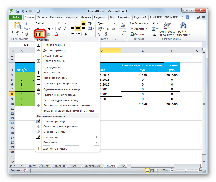
На ленте программы специальной группы инструментов для настройки границ нет. В блоке “Шрифт” представлена лишь одна кнопка, раскрывающая перечень доступных параметров.

Выбрав пункт “Другие границы” мы попадем во вкладку “Границы” окна форматирования, которую описали выше.

Заливка ячеек
Если мы перейдем во вкладку “Заливка” в окне “Формат ячеек”, то получим доступ к следующим настройкам:
- цвет фона выделенных ячеек;
- выбор узора в качестве заливки;
- цвет узора.

Отслеживать результат можно в специальном поле “Образец”.
Щелкнув по кнопке “Способы заливки” можно попасть в настройки градиентной заливки (хотя данной опцией пользуются не часто).

На панели инструментов программы, как и в случае с границами, для заливки предусмотрена только одна кнопка в группе “Шрифт” (вкладка “Главная”), нажатие на которую откроет список возможных вариантов.

При выбор пункта “Другие цвета” откроется окно в котором мы можем более детально настроить цвет в одной из двух вкладок – “Цвет” или “Спектр”.

Защита данных
С помощью данной функции можно защитить содержимое ячеек, поэтому она также доступна в окне форматирования в отдельно вкладке.
Здесь мы можем путем установки галочки:
- скрыть формулы;
- защитить ячейки.

Данные опции работают только после защиты листа. Более подробно ознакомиться с тем, как защитить данные в Эксель можно в нашей статье – “Как поставить пароль для защиты файла в Excel: книга, лист”.
На панели инструментов найти эти опции можно в группе “Ячейки” (вкладка “Главная”), нажав кнопку “Формат”.

В открывшемся списке представлен блок под названием “Защита”. Также здесь есть возможность сразу включить защиту листа. Если нужно перейти в окно “Формат ячеек”, следует нажать на одноименную кнопку.

Заключение
В Эксель пользователю предлагается обширный перечень инструментов для настройки внешнего вида таблицы, а также, определения типа данных, что крайне важно для того, чтобы программа правильно распознавала их. Большинство популярных настроек вынесено на ленту программы во вкладку “Главная”. Для более детальных настроек нужно воспользоваться окном форматирования ячеек, которое запускается через контекстное меню выделенных элементов.
Application examples of formatting Excel data of various types for computationally intensive calculations.
Changing of cells format in data tables
 Format Painter in Excel for table layout.
Multiple copies of table cell formats on multiple sheets using the Format Painter tool. Copying the width of columns and rows of a sheet.
 Influence of the cell format on working of the SUM function.
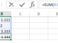
The possible errors in the summation, where there is a comma instead of a dot. Quick search of incorrect fractional numbers. Automatic assignment of the cell formats with the SUMM function.
 Transfer of data from one Excel table to another one.
You can transfer table data within one sheet, as well as to another sheet or to another file. In this case, you can copy either the entire table, or its individual values, properties or parameters.
Try it!
- Select a cell within your data.
- Select Home > Format as Table.
- Choose a style for your table.
- In the Create Table dialog box, set your cell range.
- Mark if your table has headers.
- Select OK.
Contents
- 1 Why is format as table not working?
- 2 How do you convert a table format?
- 3 How do I convert text to a table in Excel?
- 4 How do I continue a Table format in Excel?
- 5 How do I extend a formatted Table in Excel?
- 6 How do I turn a table into a column in Excel?
- 7 How do I convert a table back to normal in Excel?
- 8 How do I edit a table in Excel?
- 9 How do you convert data into a Table?
- 10 How do I convert a text file to a Table?
- 11 How do I make a Table?
- 12 How do you create a format in Excel?
- 13 Why is my table not formatting in Excel?
- 14 How do you format data in Excel?
- 15 How do I create a dynamic table in Excel?
- 16 How do I create a multi column table in Excel?
- 17 How do I convert a table to a grid in Excel?
- 18 How do I copy a table into a cell in Excel?
- 19 How do you Deduplicate in Excel?
- 20 What is the quickest way to change the format of a table?
Why is format as table not working?
If applying table styles is not working, the range was probably already formatted before you converted it to a table. (Table formatting doesn’t override normal formatting.) To clear the existing background fill colors, select the entire table and choose Home> Font> Fill Color> No Fill.
How do you convert a table format?
Microsoft Word – Convert a Table to Text
- Select the rows or table you want to convert.
- Under the Table Tools tab, select the Layout tab.
- Select Convert to Text.
- Select what you want to separate the text with: Paragraph marks, Tabs, Commas, or Other.
- Select OK.
How do I convert text to a table in Excel?
Select the text that you want to convert, and then click Insert > Table > Convert Text to Table. In the Convert Text to Table box, choose the options you want. Under Table size, make sure the numbers match the numbers of columns and rows you want. In the Fixed column width box, type or select a value.
How do I continue a Table format in Excel?
On the Home tab, in the Styles group, click Format as Table. Click the table style that you want to use. Tips: Auto Preview – Excel will automatically format your data range or table with a preview of any style you select, but will only apply that style if you press Enter or click with the mouse to confirm it.
How do I extend a formatted Table in Excel?
Resize a table by adding or removing rows and columns
- Click anywhere in the table, and the Table Tools option appears.
- Click Design > Resize Table.
- Select the entire range of cells you want your table to include, starting with the upper-leftmost cell.
- When you’ve selected the range you want for your table, press OK.
How do I turn a table into a column in Excel?
Select the table you want to transform into a single column. Click on Copy on the left-hand side of the “Professor Excel”-ribbon. Select the first cell from which Professor Excel should paste the columns underneath. Click on “Paste to Single Column” on the “Professor Excel” ribbon.
How do I convert a table back to normal in Excel?
If you need to convert the table back to the normal data range, Excel also provides an easy way to deal with it.
- Select your table range, right click and select Table > Convert to Range from the context menu.
- Tip: You can also select the table range, and then click Design > Convert to Range.
How do I edit a table in Excel?
Modifying tables
- Select any cell in your table. The Design tab will appear on the Ribbon.
- From the Design tab, click the Resize Table command. Resize Table command.
- Directly on your spreadsheet, select the new range of cells you want your table to cover. You must select your original table cells as well.
- Click OK.
How do you convert data into a Table?
Convert Data Into a Table in Excel
- Open the Excel spreadsheet.
- Use your mouse to select the cells that contain the information for the table.
- Click the “Insert” tab > Locate the “Tables” group.
- Click “Table”.
- If you have column headings, check the box “My table has headers”.
How do I convert a text file to a Table?
How to Convert Text to a Table in Word
- Open the document you want to work in or create a new document.
- Select all the text in the document and then choose Insert→Table→Convert Text to Table. You can press Ctrl+A to select all the text in the document.
- Click OK.
- Save the changes to the document.
How do I make a Table?
For a basic table, click Insert > Table and move the cursor over the grid until you highlight the number of columns and rows you want. For a larger table, or to customize a table, select Insert > Table > Insert Table.
How do you create a format in Excel?
Apply a custom number format
- Select the cell or range of cells that you want to format.
- On the Home tab, under Number, on the Number Format pop-up menu. , click Custom.
- In the Format Cells dialog box, under Category, click Custom.
- At the bottom of the Type list, select the built-in format that you just created.
- Click OK.
Why is my table not formatting in Excel?
The reason this happens is because the number formatting was NOT applied to all of the cells in the column at the same time. If you apply number formatting to one cell, then apply the same format to the rest of the cells in the column later, the Table does NOT set that as the formatting for the entire column.
How do you format data in Excel?
Formatting text and numbers
- Select the cells(s) you want to modify. Selecting a cell range.
- Click the drop-down arrow next to the Number Format command on the Home tab. The Number Formatting drop-down menu will appear.
- Select the desired formatting option.
- The selected cells will change to the new formatting style.
How do I create a dynamic table in Excel?
#1 – Using Tables to create Dynamic Tables in Excel
- Select the data, i.e., A1:E6.
- In the Insert tab, click on Tables under the tables section.
- A dialog box pops up.
- Our Dynamic Range is created.
- Select the data and in the Insert Tab under the excel tables section, click on pivot tables.
How do I create a multi column table in Excel?
How to combine two or more columns in Excel
- In Excel, click the “Insert” tab in the top menu bar.
- In the “Create Table” dialog box that pops up, edit the formula so that only the columns and rows that you want to combine are used in the table.
How do I convert a table to a grid in Excel?
Choose Cross table to list option under Transpose type. button under Source range to select the data range that you want to convert. button under Results range to select a cell where you want to put the result. With this utility, you also convert flat list table to 2-dimensional cross table.
How do I copy a table into a cell in Excel?
Copy a Word table into Excel
- In a Word document, select the rows and columns of the table that you want to copy to an Excel worksheet.
- To copy the selection, press CTRL+C.
- In the Excel worksheet, select the upper-left corner of the worksheet area where you want to paste the Word table.
- Press CRL+V.
How do you Deduplicate in Excel?
Remove duplicate values
- Select the range of cells that has duplicate values you want to remove. Tip: Remove any outlines or subtotals from your data before trying to remove duplicates.
- Click Data > Remove Duplicates, and then Under Columns, check or uncheck the columns where you want to remove the duplicates.
- Click OK.
What is the quickest way to change the format of a table?
If you don’t like the default table format, you can easily change it by selecting any of the inbuilt Table Styles on the Design tab. The Design tab is the starting point to work with Excel table styles. It appears under the Table Tools contextual tab, as soon as you click any cell within a table.
Spreadsheets are often seen as boring and pure tools of utility. It’s true that they’re useful, but that doesn’t mean that we can’t bring some style and formatting to our spreadsheets.


Good formatting helps your user find meaning in the spreadsheet without going through each and every individual cell. Cells with formatting will draw the viewer’s attention to the important cells.
In this tutorial, we’re going to dive deep into Microsoft Excel spreadsheet formatting. I’ll show you some of the easiest ways to bring formatting to your spreadsheet with just a few clicks.
How to Format an Excel Spreadsheet (Watch & Learn)
If you want a guided walk through of using Excel formatting, check out the screencast below. I’ll show you many of my favorite tricks for bringing meaning to my spreadsheets. Adding style makes a spreadsheet easier to read and less prone to mistakes, and I’ll show you why in this screencast.
Read on to find out more about the tools that you can use to change the look and feel of an Excel spreadsheet.
Format Based on Cell Type
As you probably know, Excel spreadsheets can contain a variety of data ranging from simple text to complex formulas. These spreadsheets can become complex and used in important decisions.
Formatting Excel spreadsheets isn’t just about making them «pretty.» It’s about using the built-in styles to add meaning. A spreadsheet user should be able to glance at a cell and understand it without having to look at each and every formula.
Above all, styles should be applied consistently. One idea is to use yellow shading each time you’re using a calculation. This helps the user know that the cell’s value could change based upon other cells.
Let’s learn more about the tools you can use to add meaning to your spreadsheet.
How to Use Elements of Style
When you’re thinking about styling a spreadsheet, it helps to know the tools that you can use to add style. Basically, what tools change the look of a spreadsheet? Let’s walk through how to use some of the most popular styling tools.
1. Use Bold, Italic, and Underline
These are the most basic tweaks that you can use, and you’ve probably seen them in practically every app with text editing, like Microsoft Word or Apple Pages.
To apply any of these effects, simply highlight the cells that you want to apply the effects to, and then click on the icons on the Font section of the Home tab.
You probably already know what these three tools do, but how should you use them in a spreadsheet? Here are some ideas on how you can apply those styles:
- Bold. Draw attention to key cells using bold formatting. Apply bold to totals, key assumptions in your math, and conclusion cells.
- Italic. I like to use this style for notes or any text that should be less obvious, or build to a larger subtotal.
- Underline. Adding an underline is ideal for a summary cell, like a subtotal or conclusion.
In the example below, you can see a simple financial statement for a freelancer, before and after I apply basic formatting. The combination of bold, italic, and underline effects really make the information more readable.


2. Apply Borders
Borders help to segment your data and wall it off from other sections of data in your spreadsheet. Excel’s border tool can apply a variety of borders, but is a bit tricky to get started with.
First, start off by highlighting the cells that you want to apply a border to. Then, find the Borders dropdown menu and choose one of the built-in styles.


As you can see from the dropdown options, there are many options for applying borders. Simply click on one of these border options to apply it to cells.
One of my favorite border styles is the Top and Double Bottom Border style. This is ideal particularly for financial data when you’ve got a «grand total.»
Another option is to change the weight and color of the border. With the bordered cells selected, return to the Borders dropdown menu. The Line Color and Line Style settings can be used to tweak the style of borders.


Thick borders are ideal for setting a boundary for header columns, or the subtotal at the bottom of your data.
3. Use Shading
Shading, also often called fill, is simply a color that you apply to the background of a cell. To shade a cell, click and highlight any cells that you want to add shading too.
Then, click the arrow next to the paint bucket dropdown on the Font tab on the Home ribbon. You can pick from one of the many color thumbnails to apply it to a cell. I also will frequently use the More Colors option to open a fully-featured color selection tool. Light shades are best to keep text readable.


Again, you can highlight key data using shading. As I mentioned earlier, one idea is to use a consistent fill based on the contents of the cell, such as blue for any «input» fields where you manually type data.
Don’t overdo it with shading. With too many of these applied to your cells, it distracts from the content that’s stored inside the spreadsheet.
4. Change Alignment
Alignment refers to the way that the content in a cell is aligned to the edges. You can left align, center, or right align text. By default, content is left aligned in a cell. When you’ve got large data sets, you might want to tweak alignment to enhance readability.
One common tweak that I make is putting text on the left edge of a cell, while numeric amounts should be right-aligned. Also, column headers look great when they’re centered up at the top.


Change alignment using the three alignment buttons on the Alignment tab on Excel’s Home ribbon. You can also align content vertically, adjusting if the content aligns to the top, middle, or bottom of the cell.
How to Use Built-in Cell Styles
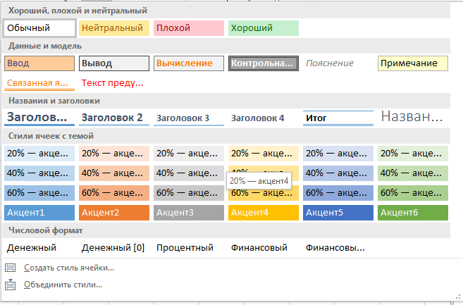
One of my favorite ways to style a spreadsheet rapidly is to use some of the built-in styles that Excel has. On the Home tab, click on the Cell Styles dropdown to apply one of the built-in styles to a cell.


Using these pre-built styles is a major time savings versus designing them from scratch. Use these as a way to take a shortcut to a more meaningful spreadsheet.
How to Achieve Faster Excel Formatting in Excel with Format Painter
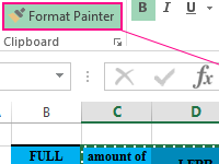
Who wants to recreate Excel cell styles over and over again? Instead of recreating the wheel for each cell, you can use the Format Painter to pick up formatting and apply it to other cells.


Start off by clicking in the cell that has the format that you want to copy. Then, find the Format Painter tool on the Home tab on Excel’s ribbon. Click on the Format Painter, then click on the cell that you want to apply the same style to.
How to Turn Off Gridlines
As you probably already know, a spreadsheet is made up of rows and columns. Rows are ruled by horizontal lines and have numbers next to them. Columns are split with vertical lines and have letters at the top to refer to them.
Where rows and columns meet, cells are formed. Cells have names for which row and column they intersect. For example, where row 4 and column B meet is called B4.
Gridlines in Excel are one of the defining features of a spreadsheet. They make it easy to follow data across the screen into a cell. These lines are imaginary and only visible on screen. However, you might want to turn off gridlines for a stylistic effect.


Print with Gridlines
What if you wanted to show gridlines throughout the spreadsheet when you print it? Instead of having to manually add borders to each and every cell, you can simply print your workbook and include those gridlines.
To turn on gridlines when printing, start by going to the Print option. Then, click on Page Setup to open the settings.
On the Sheet tab, tick the box labeled Gridlines to include gridlines when you print your Excel workbook.


Keep in mind that this option will certainly use more ink when printing. However, it also might make it easier to read your printed spreadsheet.
How to Format Excel Data as Table
One of my favorite ways to style a dataset quickly is to use the Format as Table dropdown option. With just a couple of clicks, you can transform a few rows and columns into a structured data table.


This feature works best when you already have data in a set of rows and columns and want to apply a uniform style. It’s a combination of style and functionality, as tables add other features like automatic filtering buttons.
Learn more about why tables are a great feature in the tutorial below:
How to Use Conditional Formatting in Excel
What if the format for a cell could change based on the data that’s inside of it? This feature is built into Excel and is called Conditional Formatting. It’s easier to get started with than you may think.
Imagine using Conditional Formatting to highlight the top and bottom values in your cells. It makes it easy to visually scan your data and look for key indicators.


Conditional Formatting is best used with numerical data. To get started, simply highlight a column of data and make sure that you’re on the Home tab on Excel’s ribbon.
There are a number of styles that you can choose from the Conditional Formatting dropdown menu. Each of these applies a different style of Excel formatting to your cells, but each will adapt based on the cells that you’ve highlighted.


Recap & Keep Learning
Spreadsheets are often seen as boring and pure tools of utility. Sure, they’re very useful for organizing data or making calculations. That doesn’t mean that we can’t bring some style and Excel formatting to our spreadsheets.
When we do formatting the right way, it adds a second layer of meaning to a spreadsheet. Formatting isn’t a random exercise; it’s a way of using targeted styles to signal what type of data is in a cell.
Check out these other tutorials if you want to level up your Microsoft Excel skills and master spreadsheets:
What are your favorite Excel formatting tips? How do you make sure that the right cells stand out to your user? Let me know in the comments section below.
Did you find this post useful?

I believe that life is too short to do just one thing. In college, I studied Accounting and Finance but continue to scratch my creative itch with my work for Envato Tuts+ and other clients. By day, I enjoy my career in corporate finance, using data and analysis to make decisions.
I cover a variety of topics for Tuts+, including photo editing software like Adobe Lightroom, PowerPoint, Keynote, and more. What I enjoy most is teaching people to use software to solve everyday problems, excel in their career, and complete work efficiently. Feel free to reach out to me on my website.
Formatting is one of the main processes when working with a spreadsheet. By applying formatting, you can change the appearance of tabular data, as well as set cell options. It is important to be able to implement it correctly in order to do your work in the program quickly and efficiently. From the article you will learn how to format the table correctly.
Table Formatting
Formatting is a set of actions that is necessary to edit the appearance of a table and the indicators inside it. This procedure allows you to edit the font size and color, cell size, fill, format, and so on. Let’s analyze each element in more detail.
Auto-formatting
Autoformatting can be applied to absolutely any range of cells. The spreadsheet processor will independently edit the selected range, applying the assigned parameters to it. Walkthrough:
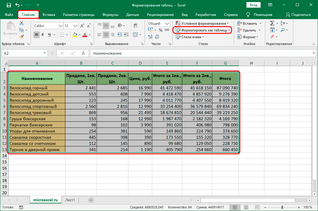
- We select a cell, a range of cells or the entire table.
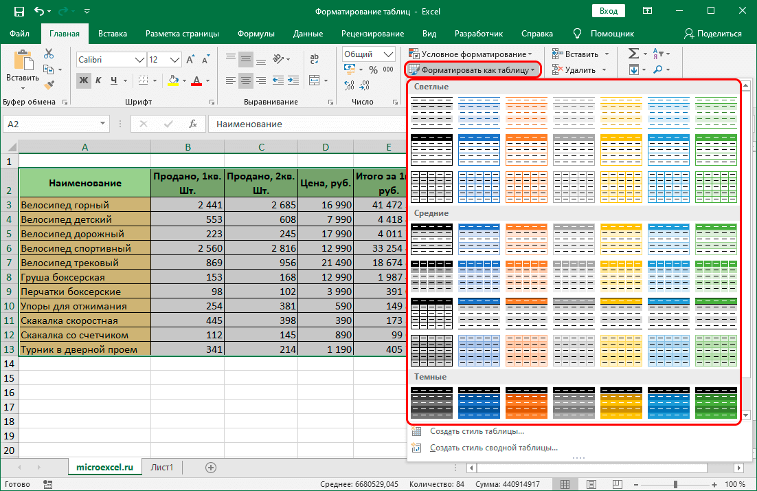
- Go to the “Home” section and click “Format as Table”. You can find this element in the “Styles” block. After clicking, a window with all possible ready-made styles is displayed. You can choose any of the styles. Click on the option you like.
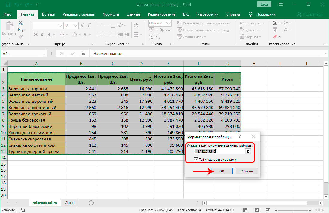
- A small window was displayed on the screen, which requires confirmation of the correctness of the entered range coordinates. If you notice that there is an error in the range, you can edit the data. You need to carefully consider the item “Table with headers.” If the table contains headings, then this property must be checked. After making all the settings, click “OK”.
- Ready! The plate has taken on the appearance of the style you have chosen. At any time, this style can be changed to another.
Switching to formatting
The possibilities of automatic formatting do not suit all users of the spreadsheet processor. It is possible to manually format the plate using special parameters. You can edit the appearance using the context menu or the tools located on the ribbon. Walkthrough:
- We make a selection of the necessary editing area. Click on it RMB. The context menu is displayed on the screen. Click on the “Format Cells…” element.
- A box called “Format Cells” appears on the screen. Here you can perform various tabular data editing manipulations.
The Home section contains various formatting tools. In order to apply them to your cells, you need to select them, and then click on any of them.
Data Formatting
The cell format is one of the basic formatting elements. This element not only modifies the appearance, but also tells the spreadsheet processor how to process the cell. As in the previous method, this action can be implemented through the context menu or the tools located in the special ribbon of the Home tab.
By opening the “Format Cells” window using the context menu, you can edit the format through the “Number Formats” section, located in the “Number” block. Here you can choose one of the following formats:
- date;
- time;
- common;
- numerical;
- text, etc.
After selecting the required format, click “OK”.
In addition, some formats have additional options. By selecting a number format, you can edit the number of digits after the decimal point for fractional numbers.
By setting the “Date” format, you can choose how the date will be displayed on the screen. The “Time” parameter has the same settings. By clicking on the “All formats” element, you can view all possible subspecies of editing data in a cell.
By going to the “Home” section and expanding the list located in the “Number” block, you can also edit the format of a cell or a range of cells. This list contains all the major formats.
By clicking on the item “Other number formats …” the already known window “Format of cells” will be displayed, in which you can make more detailed settings for the format.
Content alignment
By going to the “Format Cells” box, and then to the “Alignment” section, you can make a number of additional settings to make the appearance of the plate more presentable. This window contains a large number of settings. By checking the box next to one or another parameter, you can merge cells, wrap text by words, and also implement automatic width selection.
In addition, in this section, you can implement the location of the text inside the cell. There is a choice of vertical and horizontal text display.
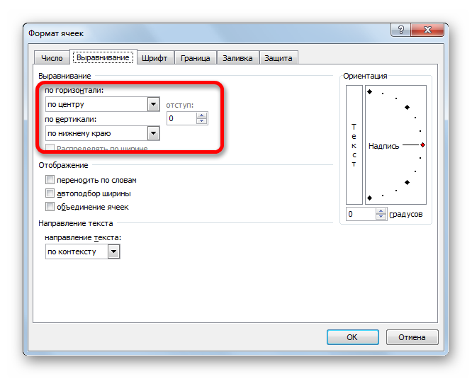
In the “Orientation” section, you can adjust the positioning angle of the text information inside the cell.
In the “Home” section there is a block of tools “Alignment”. Here, as in the “Format Cells” window, there are data alignment settings, but in a more cropped form.
Font setting
The “Font” section allows you to perform a large set of actions to edit the information in the selected cell or range of cells. Here you can edit the following:
- a type;
- the size;
- Colour;
- style, etc.
On a special ribbon is a block of tools “Font”, which allows you to perform the same transformations.
Borders and lines
In the “Border” section of the “Format Cells” window, you can customize the line types, as well as set the desired color. Here you can also choose the style of the border: external or internal. It is possible to completely remove the border if it is not needed in the table.
Unfortunately, there are no tools for editing table borders on the top ribbon, but there is a small element that is located in the “Font” block.
Filling cells
In the “Fill” section of the “Format Cells” box, you can edit the color of the table cells. There is an additional possibility of exhibiting various patterns.
As in the previous element, there is only one button on the toolbar, which is located in the “Font” block.
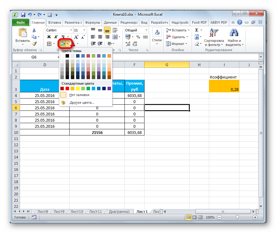
It happens that the user does not have enough standard shades to work with tabular information. In this case, you need to go to the “Other colors …” section through the button located in the “Font” block. After clicking, a window is displayed that allows you to select a different color.
Cell styles
You can not only set the cell style yourself, but also choose from those integrated into the spreadsheet itself. The library of styles is extensive, so each user will be able to choose the right style for themselves.
Walkthrough:
- Select the necessary cells to apply the finished style.
- Go to the “Home” section.
- Click “Cell Styles”.
- Choose your favorite style.
Data protection
Protection also belongs to the realm of formatting. In the familiar “Format Cells” window, there is a section called “Protection”. Here you can set protection options that will prohibit editing the selected range of cells. And also here you can enable hiding formulas.
On the tool ribbon of the Home section, in the Cells block, there is a Format element that allows you to perform similar transformations. By clicking on “Format”, the screen will display a list in which the “Protection” element exists. By clicking on “Protect sheet …”, you can prohibit editing the entire sheet of the desired document.
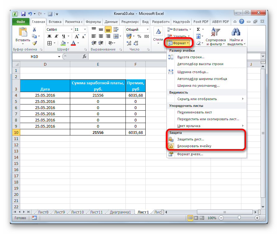
Table themes
In the spreadsheet Excel, as well as the word processor Word, you can choose the theme of the document.
Walkthrough:
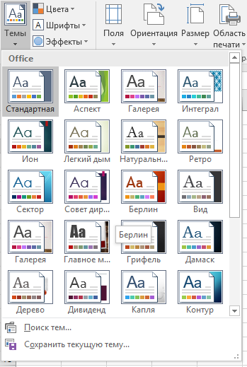
- Go to the “Page Layout” tab.
- Click on the “Themes” element.
- Choose one of the ready-made themes.
Transformation into a “Smart Table”
A “smart” table is a special type of formatting, after which the cell array receives certain useful properties that make it easier to work with large amounts of data. After the conversion, the range of cells is considered by the program as a whole element. Using this function saves users from recalculating formulas after adding new rows to the table. In addition, the “Smart” table has special buttons in the headers that allow you to filter the data. The function provides the ability to pin the table header to the top of the sheet. Transformation into a “Smart Table” is performed as follows:
- Select the required area for editing. On the toolbar, select the “Styles” item and click “Format as Table”.
- The screen displays a list of ready-made styles with preset parameters. Click on the option you like.
- An auxiliary window appeared with settings for the range and display of titles. We set all the necessary parameters and click the “OK” button.
- After making these settings, our tablet turned into a Smart Table, which is much more convenient to work with.
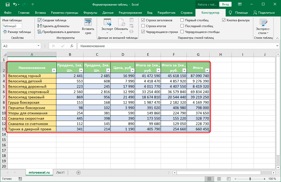
Table Formatting Example
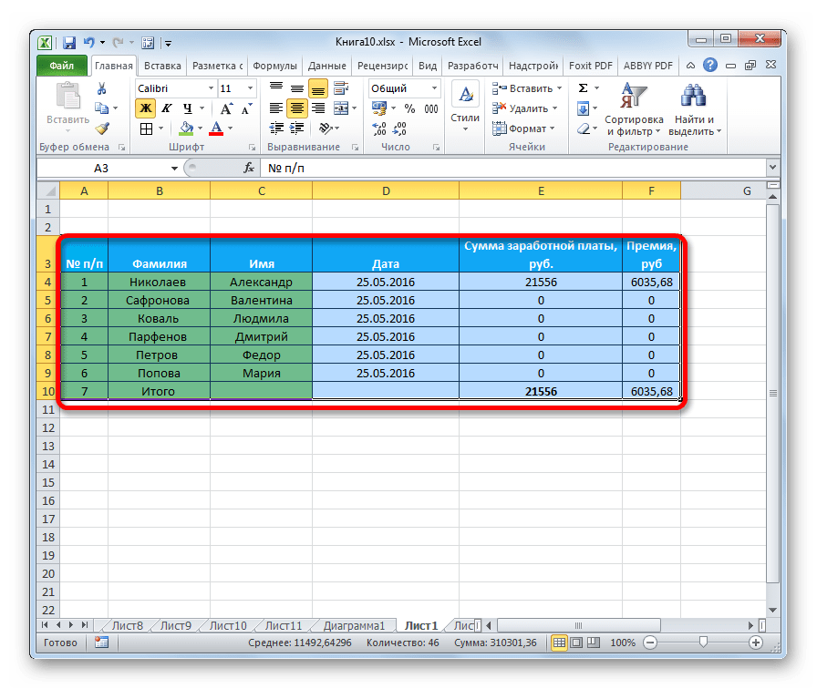
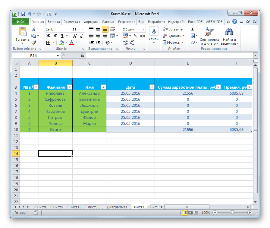
Let’s take a simple example of how to format a table step by step. For example, we have created a table like this:
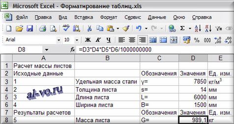
Now let’s move on to its detailed editing:
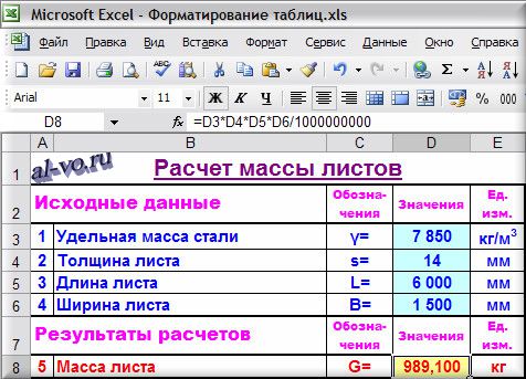
- Let’s start with the title. Select the range A1 … E1, and click on “Merge and move to the center.” This item is located in the “Formatting” section. The cells are merged and the inner text is center aligned. Set the font to “Arial”, the size to “16”, “Bold”, “Underlined”, the font shade to “Purple”.
- Let’s move on to formatting the column headings. Select cells A2 and B2 and click “Merge Cells”. We perform similar actions with cells A7 and B7. We set the following data: font – “Arial Black”, size – “12”, alignment – “Left”, font shade – “Purple”.
- We make a selection of C2 … E2, while holding “Ctrl”, we make a selection of C7 … E7. Here we set the following parameters: font – “Arial Black”, size – “8”, alignment – “Centered”, font color – “Purple”.
- Let’s move on to editing posts. We select the main indicators of the table – these are cells A3 … E6 and A8 … E8. We set the following parameters: font – “Arial”, “11”, “Bold”, “Centered”, “Blue”.
- Align to the left edge B3 … B6, as well as B8.
- We expose the red color in A8 … E8.
- We make a selection of D3 … D6 and press RMB. Click “Format Cells…”. In the window that appears, select the numeric data type. We perform similar actions with cell D8 and set three digits after the decimal point.
- Let’s move on to formatting the borders. We make a selection of A8 … E8 and click “All Borders”. Now select “Thick Outer Border”. Next, we make a selection of A2 … E2 and also select “Thick outer border”. In the same way, we format A7 … E7.
- We do color setting. Select D3…D6 and assign a light turquoise hue. We make a selection of D8 and set a light yellow tint.
- We proceed to the installation of protection on the document. We select cell D8, right-click on it and click “Format Cells”. Here we select the “Protection” element and put a checkmark next to the “Protected cell” element.
- We move to the main menu of the spreadsheet processor and go to the “Service” section. Then we move to “Protection”, where we select the element “Protect Sheet”. Setting a password is an optional feature, but you can set it if you wish. Now this cell cannot be edited.
In this example, we examined in detail how you can format a table in a spreadsheet step by step. The result of formatting looks like this:
As we can see, the sign has changed drastically from the outside. Her appearance has become more comfortable and presentable. By similar actions, you can format absolutely any table and put protection on it from accidental editing. The manual formatting method is much more efficient than using predefined styles, since you can manually set unique parameters for any type of table.
Conclusion
The spreadsheet processor has a huge number of settings that allow you to format data. The program has convenient built-in ready-made styles with set formatting options, and through the “Format Cells” window, you can implement your own settings manually.