How to format excel dates - Word и Excel - помощь в работе с программами

Format numbers as dates or times

Excel for Microsoft 365 Excel for Microsoft 365 for Mac Excel for the web Excel 2021 Excel 2021 for Mac Excel 2019 Excel 2019 for Mac Excel 2016 Excel 2016 for Mac Excel 2013 Excel 2010 Excel 2007 Excel for Mac 2011 More…Less

When you type a date or time in a cell, it appears in a default date and time format. This default format is based on the regional date and time settings that are specified in Control Panel, and changes when you adjust those settings in Control Panel. You can display numbers in several other date and time formats, most of which are not affected by Control Panel settings.

Display numbers as dates or times

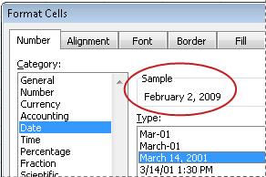
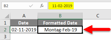
You can format dates and times as you type. For example, if you type 2/2 in a cell, Excel automatically interprets this as a date and displays 2-Feb in the cell. If this isn’t what you want—for example, if you would rather show February 2, 2009 or 2/2/09 in the cell—you can choose a different date format in the Format Cells dialog box, as explained in the following procedure. Similarly, if you type 9:30 a or 9:30 p in a cell, Excel will interpret this as a time and display 9:30 AM or 9:30 PM. Again, you can customize the way the time appears in the Format Cells dialog box.

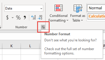
On the Home tab, in the Number group, click the Dialog Box Launcher next to Number.

You can also press CTRL+1 to open the Format Cells dialog box.
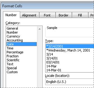
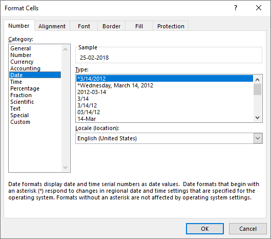
In the Category list, click Date or Time.
In the Type list, click the date or time format that you want to use.

Note: Date and time formats that begin with an asterisk (*) respond to changes in regional date and time settings that are specified in Control Panel. Formats without an asterisk are not affected by Control Panel settings.
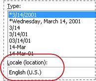
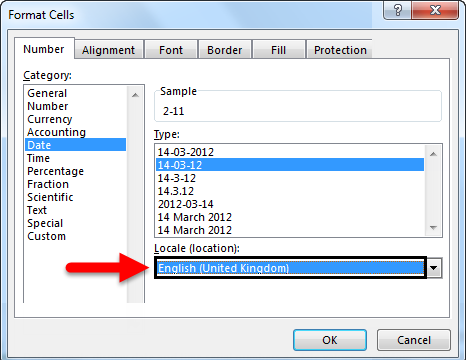
To display dates and times in the format of other languages, click the language setting that you want in the Locale (location) box.

The number in the active cell of the selection on the worksheet appears in the Sample box so that you can preview the number formatting options that you selected.

Top of Page

Create a custom date or time format

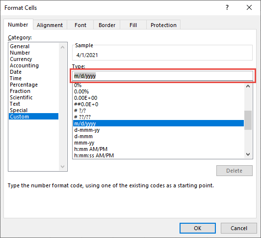
On the Home tab, click the Dialog Box Launcher next to Number.

You can also press CTRL+1 to open the Format Cells dialog box.
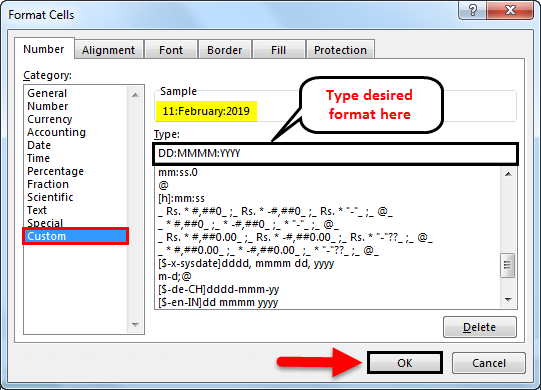
In the Category box, click Date or Time, and then choose the number format that is closest in style to the one you want to create. (When creating custom number formats, it’s easier to start from an existing format than it is to start from scratch.)
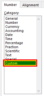
In the Category box, click Custom. In the Type box, you should see the format code matching the date or time format you selected in the step 3. The built-in date or time format can’t be changed or deleted, so don’t worry about overwriting it.
In the Type box, make the necessary changes to the format. You can use any of the codes in the following tables:

Days, months, and years

To display	Use this code
Months as 1–12	m
Months as 01–12	mm
Months as Jan–Dec	mmm
Months as January–December	mmmm
Months as the first letter of the month	mmmmm
Days as 1–31	d
Days as 01–31	dd
Days as Sun–Sat	ddd
Days as Sunday–Saturday	dddd
Years as 00–99	yy
Years as 1900–9999	yyyy

If you use «m» immediately after the «h» or «hh» code or immediately before the «ss» code, Excel displays minutes instead of the month.

Hours, minutes, and seconds

To display	Use this code
Hours as 0–23	h
Hours as 00–23	hh
Minutes as 0–59	m
Minutes as 00–59	mm
Seconds as 0–59	s
Seconds as 00–59	ss
Hours as 4 AM	h AM/PM
Time as 4:36 PM	h:mm AM/PM
Time as 4:36:03 P	h:mm:ss A/P
Elapsed time in hours; for example, 25.02	[h]:mm
Elapsed time in minutes; for example, 63:46	[mm]:ss
Elapsed time in seconds	[ss]
Fractions of a second	h:mm:ss.00

AM and PM If the format contains an AM or PM, the hour is based on the 12-hour clock, where «AM» or «A» indicates times from midnight until noon and «PM» or «P» indicates times from noon until midnight. Otherwise, the hour is based on the 24-hour clock. The «m» or «mm» code must appear immediately after the «h» or «hh» code or immediately before the «ss» code; otherwise, Excel displays the month instead of minutes.

Creating custom number formats can be tricky if you haven’t done it before. For more information about how to create custom number formats, see Create or delete a custom number format.

Top of Page

Tips for displaying dates or times

To quickly use the default date or time format, click the cell that contains the date or time, and then press CTRL+SHIFT+# or CTRL+SHIFT+@.
If a cell displays ##### after you apply date or time formatting to it, the cell probably isn’t wide enough to display the data. To expand the column width, double-click the right boundary of the column containing the cells. This automatically resizes the column to fit the number. You can also drag the right boundary until the columns are the size you want.
When you try to undo a date or time format by selecting General in the Category list, Excel displays a number code. When you enter a date or time again, Excel displays the default date or time format. To enter a specific date or time format, such as January 2010, you can format it as text by selecting Text in the Category list.
To quickly enter the current date in your worksheet, select any empty cell, and then press CTRL+; (semicolon), and then press ENTER, if necessary. To insert a date that will update to the current date each time you reopen a worksheet or recalculate a formula, type =TODAY() in an empty cell, and then press ENTER.

Need more help?

You can always ask an expert in the Excel Tech Community or get support in the Answers community.

Need more help?

Want more options?

Explore subscription benefits, browse training courses, learn how to secure your device, and more.

Communities help you ask and answer questions, give feedback, and hear from experts with rich knowledge.

Источник

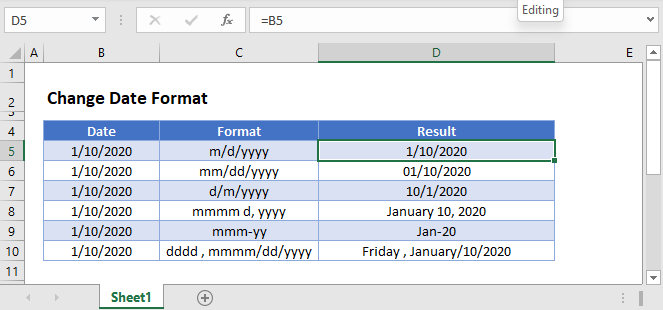
In this guide, we’ll learn how to change date format in Excel. Date and Time data is an integral part of any statistical document or sheet. It is important to accurately track and analyze events, sales, figures, and others.

By convention, Excel uses a general data format that may be as per your need. But in most cases, that format may need to be customized.

Changing the format of Date in a particular cell or all the cells in your Excel sheet is an easy process and doesn’t require any complex methodologies. Excel provides a wide range of formatting options based on Location and Languages which helps in better date formatting in native language and style. Also, For some Languages there is also features to select from different Calendar types.

Follow the below step-by-step tutorial to change date format in Excel quickly and easily.

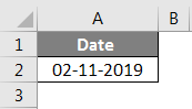
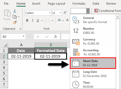
Step 1. Select the range of cells containing the date

To start with, select the cell values where want to change the date format, as shown in the image below.

Sample selection of dates in default formatting option

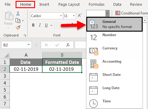
Step 2. Go to Number Format dropdown

To select ‘Number Format’, go to ‘Home‘ in the option menu and look for Number Format, as shown below
Then from the drop-down menu, select ‘More Number Formats‘ to reveal the ‘Number Format’ dialogue menu.

Select Number Format

Alternatively, you may directly go to Number Format, by right-clicking on the selected cell/s
Click on ‘Number Format’.

Right Click and select Number Format

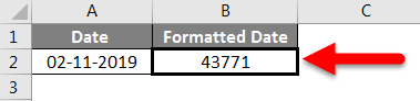
Step 3. Choose Date

From the Category menu on the right, choose ‘Date‘.

Format Date option menu

Now, to apply any date formatting type, select it from the right panel of the pop-up menu of Number Format. Click on ‘OK‘ to apply the formatting to the selected cell/s.

Note: You may check the date format implementation in the ‘Sample‘ at the top of the menu option

Choose the Date Type

The general option type to choose from a variety of Date Formatting options. Scroll down in this section to reveal a plethora of options for formatting, ranging from date, text (month name), year, and others.

This option can be perceived as the display menu, as the formatting options in this will keep on changing as per the selection in Locale(Location) and Calendar type.

General Date Formatting

Choose the Locale (location)

This option features the Location or Language options to help format the date accordingly. This option is probably the most used option as users require to format the date according to their or audience preference as per the native formatting style, based on language and location.

Choose any language or Location from this options menu. After selecting, all the supported date format options available for that particular locale will be available for selecting in the above Type menu.

selecting locale (language) in date formatting

Choose the type of calendar

This option reveals different calendar types available based on the Locale(Location) selected from the above option menu. This formatting option is only available for certain Locale and not all.

As shown in our example below, the variety of calendar types available for selection are only available for the Locale (location) selected (here, Arabia), for other locales the calendar type might be different or not at all present.

Selecting Calendar type in Date Formatting

To apply selected formatting, you will need to click ‘OK‘ after selection to apply to your dates.

Conclusion

That’s It! You can now easily convert your dates to your desired format style easily.

We hope you learned and enjoyed this lesson and we’ll be back soon with another awesome Excel tutorial at QuickExcel!

Источник

What is a date in Excel?

A date is a number! And like any number (currency, percentage, decimal, …), you can customize your date format 👍

Dates are whole numbers

Usually, when you insert a date in a cell it is displayed in the format dd/mm/yyyy or mm/dd/yyyy.

Let’s say you have the date 01/01/2016 in a cell. If you change the cell’s format to Standard, the cell displays 42370 😕🤔

Explanation of the numbering

In Excel, a date is the number of days since 01/01/1900 (the first date in Excel).

So 42370 is the number of days between 01/01/1900 and 01/01/2016.

Date format

Dates can be displayed in different ways using the following 2 options (available in the Number Format dropdown in the main menu):

Short Date
Long Date

How to customize a date?

To customize a date:

Open the dialog box Custom Number (with the shortcut Ctrl + 1 or by clicking on the menu More number formats at the bottom of the number format dropdown)

In this dialog box, you select ‘Custom‘ in the Category list and write the date format code in ‘Type‘.

To format a date, you just write the parameter d, m or y a different number of times. For example,

dd/mm/yyyy will display 01/01/2016
dd mmm yyyy => 01 Jan 2016
mmmm yyyy => January 2016
dddd dd => Friday 01

In function of your language , the letter could be different:

t for «tag» (day) in German
j for «jour» (day) in French
a for «año» (year) in Spanish

Don’t write text in your cell !!!

With dates, one of the most common mistakes is to write text inside the format code (1 January 2016 for example). Never do this in Excel ⛔⛔⛔

If you do this, the contents of the cell will be Text and not a number

In Excel, text is always displayed on the left of a cell.
A number or a date is displayed on the right.

If you want to display the month in letters, just change the month format of your date.

Different examples of custom date

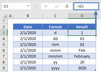
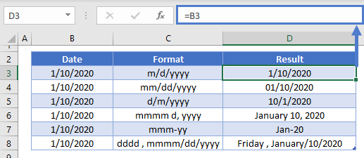
The following document shows you the same date but in different formats. The code for each date is in column A.

Different writing of dates according to the format code

In the following document, you can see the impact of each format on the same date.

Источник

What is the Date Format in Excel?

In Excel, a date is displayed according to the format selected by the user. One can choose from the different formats available or create a customized format according to the requirement. The default date format is specified in the “Control Panel” of the system. However, it is possible to change these default settings.

For example, the date 01/01/2021 corresponds to the format dd/mm/yyyy. If the format is changed to d-mmm-yyyy, the date becomes 1-Jan-2021.

We can change the date format in Excel either from the “Number Format” of the “Home” tab or the “Format Cells” option of the context menu.

In Excel for Windows, 1900 is the default date system. Whereas, in Excel for Mac, 1904 is the default date system. Both these systems store the dates as consecutive numbers having a difference of 1. These numbers are known as serial values or serial numbers. The reason dates are stored as serial numbers is to facilitate calculations.

In the 1900 date system, the first date that Excel recognizes is January 1, 1900. This date is stored as the number 1 in Excel. Consequently, the number 2 represents January 2, 1900. The last date recognized by Excel is December 31, 9999. It is represented by the serial number 2958465. Date before 1900 or after 9999 is identified as a text value by Excel.

Dates are stored only as positive integers in the 1900 date system. However, to display negative numbers as negative dates, one needs to switch to the 1904 date system.

In the 1904 date system, 0 represents January 1, 1904, and -1 means January -2, 1904. The number 1 represents January 2, 1904. The last date recognized by Excel (in the 1904 date system) is December 31, 9999, represented by the serial number 2957003.

In this article, we follow the 1900 date system.

What is theDate Format in Excel?
- Code of Date Format in Excel
- How to Change Date Format in Excel?
  - Example #1–Apply Default Format of Long Date in Excel
  - Example #2–Change the Date Excel Format Using “Custom” Option
  - Example #3–Apply Different Types of Customized Date Formats in Excel
  - Example #4–Convert Text Values Representing Dates to Actual Dates
  - Example #5–Change the Date Format Using “Find and Replace” Box
- Frequently Asked Questions
- Recommended Articles

Code of Date Format in Excel

A code (like dd-mm-yyyy) is a representation of a day (d), month (m), and year (y). We can change the appearance of the date by changing the specified code.

The different codes, their explanation, and output (for days, months, and years) have been presented in the following images.

Notations for a Day

Notations for a Month

Notations for a Year

How to Change Date Format in Excel?

Here we look at some of the date format examples in Excel and how to change them.

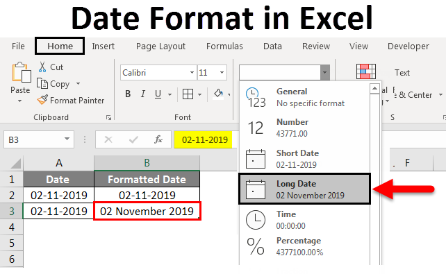
Example #1–Apply Default Format of Long Date in Excel

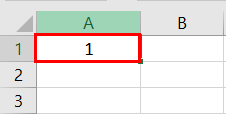
The following image shows a number in cell A1. We want to know the date represented by this number. The output should be in the long date format of Excel.

The steps to know the date represented by the number in cell A1 are listed as follows:

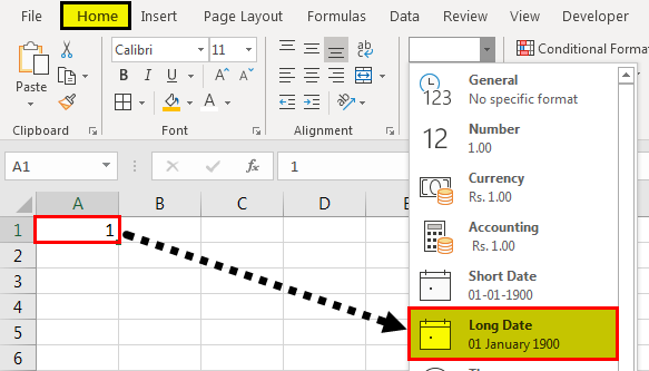
We must first select cell A1. Then, from the “Home” tab, click the “Number Format” drop-down appearing in the “Number” section. Next, select “Long Date,” shown in the following image.
The output is shown in the following image. The long date format displayed is dd mmmm yyyy. Hence, the number 1 represents the date 01 January 1900 in the long date format.
Note: The short and long dates appear as set in the “Control Panel.” Click “Clock, Language, and Region” in the “Control Panel” to change these default date formats. After that, click “Change date, time, or number formats.” Make the desired changes and click “OK.”

Likewise, had there been 2 in cell A1, the long date format would have been 02 January 1900. The number 3 would have been displayed as 03 January 1900 in the long date format.

Note: To switch to the 1904 date system, we must select “Advanced” from the “Options” of the “File” tab. Under “When calculating this workbook,” select “use 1904 date system” and click “OK.”

You can download this Change Date Format Excel Template here – Change Date Format Excel Template

Example #2–Change the Date Excel Format Using “Custom” Option

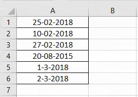
The following image shows some dates in the range A1:A6. These dates are in the format dd-mm-yyyy. We want to change their format to dd-mmmm-yyyy.

For instance, the date in cell A1 should appear as 25-February-2018. We may use the “Custom” option of the “Format Cells” dialog box.

The steps to change the date format in Excel are listed as follows:

Step 1: We need to select all the dates of the range A1:A6. The same is shown in the following image.

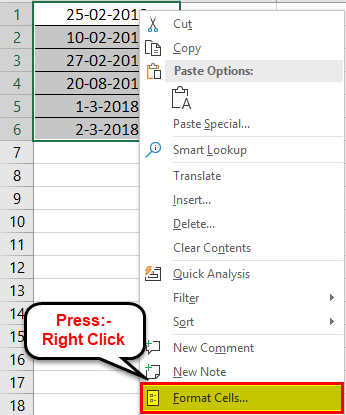
Step 2: We must right-click the selection and choose “Format Cells” from the context menu. Alternatively, we may also press the keys “Ctrl+1” together.

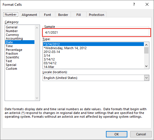
Step 3: The “Format Cells” window opens, as shown in the following image.

Note: The default short date and long date formats are marked with an asterisk (*) in the box under “type.” The short date is 3/14/2012 (m/dd/yyyy), and the long date is Wednesday, March 14, 2012 (dddd, mmmm dd, yyyy).

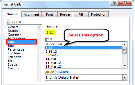
Step 4: From the “Number” tab, we need to select “Custom” under “Category.” The categories are shown on the left side of the “Format Cells” window.

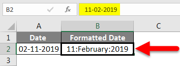
Step 5: Under “Type,” we must insert the required date format. Either type the format (dd-mmmm-yyyy) or select it from the various options displayed in the box below “Type.”

Once the format has been entered, check the preview of the first date (of the range A1:A6) under “Sample.” The same is shown in the following image. Click “OK” in the “Format Cells” window if the date preview looks good.

Note 1: The date under “Sample” is displayed according to the format specified under “Type.”

Note 2: While creating custom date formats, we can use a forward slash (/), hyphen (-), comma (,), space ( ), etc.

Step 6: The output is shown in the following image. All dates of the range A1:A6 have been converted to the format dd-mmmm-yyyy. However, the Excel formula bar can still see the default date format. This default format corresponds with the short date set in the “Control Panel.”

Example #3–Apply Different Types of Customized Date Formats in Excel

The next image shows certain dates in the range A1:A6. At present, the date format is dd-mm-yyyy.

We want to apply four different formats to these dates. For using each format, the common steps to be performed are given as follows:

First, we must select the range A1:A6.
Then, right-click the selection and choose “Format Cells.”
After that, from the “Number” tab, select “Custom” under “Category.”

Further, under each format, the additional steps to be performed followed by two images are given.

Format 1: dd-mmm-yyyy

In the “Custom” option of the “Number” tab, select the format “dd-mmm-yyyy” under “Type.”
Click “Ok.”

The output is given in the following image. All dates are displayed according to the format dd-mmm-yyyy. The hyphen is the separator between the day, month, and year in this format.

Format 2: dd mmm yyyy

We must select the format “dd mmm yyyy” under “Type” of the “custom” option.
Click “Ok.”

The output is given in the following image. All dates are converted to the format dd mmm yyyy. The space is the only separator between the day, month, and year in this format.

Format 3: ddd mmm yyyy

In the “Custom” option, select the format “ddd mmm yyyy” under “Type.”
Click “Ok.”

The output is given in the following image. The dates are shown in the format ddd mmm yyyy. The day and the month are displayed in their short notations in this format.

Format 4: dddd mmmm yyyy

From the “Custom” option of the “Number” tab, select “dddd mmmm yyyy” under “Type.”
Click “Ok.”

The output is given in the following image. All dates have been converted to the format dddd mmmm yyyy. The date, month, and year are displayed in their respective full forms in this format.

It must be observed that the date format changes as per the style set by the user. Therefore, the user can select a date format according to their convenience.

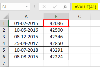
Example #4–Convert Text Values Representing Dates to Actual Dates

The following image shows a list of dates in the range A1:A6. At present, these dates are appearing as text values. We want to convert these text values to dates having the format dd-mmm-yyyy.

The steps to convert text values to dates having the given format are listed as follows:

Step 1: First, enter the following formula in cell B1.

“=VALUE(A1)”

Then, press the “Enter” key.

Note 1: The VALUE functionIn Excel, the value function returns the value of a text representing a number. So, if we have a text with the value $5, we can use the value formula to get 5 as a result, so this function gives us the numerical value represented by a text.read more returns the numeric form of a text string that represents a number. In other words, it converts a number looking like the text into an actual number.

Note 2: Instead of the VALUE function, one can also use the DATEVALUE functionThe DATEVALUE function in Excel shows any given date in absolute format. This function takes an argument in the form of date text normally not represented by Excel as a date and converts it into a format that Excel can recognize as a date.read more of Excel. The latter converts a date stored as text to a serial number. This serial number is recognized as a date by Excel.

Step 2: We must select cell B1 and drag the fill handle until cell B6. The output is shown in the following image. All text values (A1:A6) have been converted to numbers (in the range B1:B6).

Ideally, the text string in Excel is left-aligned while the number string is right-aligned. However, we have centrally aligned both the ranges (A1:A6 and B1:B6).

Note: When text strings representing dates have been converted to serial values (or dates), we can use them for performing different calculations like addition, subtraction, and so on.

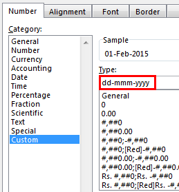
Step 3: To view the obtained serial numbers (in column B) as dates, apply the required format. We must select the range B1:B6, right-click and choose “Format Cells.”

In the “Number” tab, select the option “Custom.” Then, under “Type,” enter or choose the format “dd-mmm-yyyy.” The same is shown in the following image.

If the sample date looks alright, click “OK.”

Step 4: The output is shown in the following image. Hence, all text values (of column A) have been converted to valid dates (in column B) having the format dd-mmm-yyyy.

Note: To ensure that a value is recognized as a date by Excel, check for the following signs:

The dates are right-aligned as they are numerical values.
If two or more dates are selected, the status bar (at the bottom of the worksheet) shows the count, average, numerical count, and sum. In addition, it may display one or more options according to the Excel version.

If a value is a text string, it would be left-aligned, and the status bar will show only the count.

Often, the Excel date format needs to be changed (from text to dates) when data is downloaded (or copied and pasted) from the web. That is because, in such instances, the dates may not be displayed as numbers.

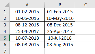
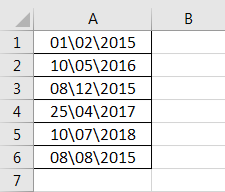
Example #5–Change the Date Format Using “Find and Replace” Box

The following image shows some text values representing dates in the range A1:A6. The days, months, and numbers have been separated with a backslash. That is because we want to perform the following tasks:

Replace all the backslashes () with forwarding slashes (/) by using the “Find and Replace” dialog box.
Convert text values representing dates to actual dates.

The steps to perform the given tasks are listed as follows:

Step 1: We must press the keys “Ctrl+H” together. Then, the “find and replace” dialog box opens, as shown in the following image.

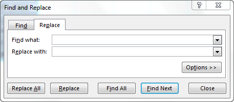
Step 2: Type a backslash in the “Find what” box (). In the “Replace with” box, type a forward slash (/).

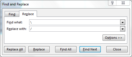
Step 3: Next, we must click “Replace All.” Excel shows a message stating the number of replacements it has made. Click “OK” to proceed. The final output is shown in the following image.

Hence, all backslashes have been replaced with forwarding slashes. With this replacement, the text values representing dates have automatically been converted to actual dates by Excel.

Since column A was aligned centrally from the beginning, this alignment is retained even after the values are converted to dates.

Frequently Asked Questions

1. How can the date format in Excel be changed?

The steps to change the date format in Excel are listed as follows:
The steps to change the date format in Excel are listed as follows:

a. Select the cell containing the date. If the date format of a range needs to be changed, select the entire range.
b. Right-click the selection and choose “Format Cells” from the context menu. Alternatively, press the keys “Ctrl+1” together.
c. IIn the “Number” tab, select the option “Date.” Next, select the required date format under “Type.”
d. Check the preview (of the first date of the selected range) under “Sample.” If the preview is good, click “OK.”

The date format of the selected cell or cells (selected in step a) is changed.

Note 1: The required date format may not be available under the “Date” option’s “Type.” If it is not available, select “Custom” as the “category” from the “Number” tab. Then, type the required date format under “Type” and click “OK.”

Note 2: If the selected cell (selected in step a) contains a text string representing a date, convert this string to date first. Then change the format to the desired date format.

2. How to change the date format permanently in Excel?

To change a date format permanently, one needs to make changes to the date formats of the “Control Panel.” That is because the short and long date formats of Excel reflect the date settings of the “Control Panel.”

The steps to change the date settings of the “Control Panel” are listed as follows:

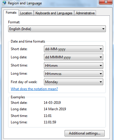
We must open the “Control Panel” first from the “Start” menu.
b. In the “Clock, Language, and Region” category, click “Change date, time, or number format.” It is available under the “Region and Language” option.
c. The “Region and Language” or “Region” dialog box opens. Under “Format,” we must select the region.
d. Enter the required short and long date formats under “Date and Time Formats.” To enter customized short and long date formats, click “Additional Settings.” The “Customize Format” dialog box opens. Make the changes in the “Date” tab and click “OK.”
e. Check the preview under “Examples” at the bottom of the “Region and Language” box. If the preview is alright, click “OK.”

The default date settings have been changed. Now, we should enter a date in any format in Excel. Then select the short or the long date format from the “Number Format” (in the “Number” section) of the “Home” tab.
The dates will appear in the format set in the “Control Panel.” So, the user need not change the format of each date manually.

3. How to change a date to a text string in Excel?

Let us change the date 22/1/2019 in cell A1 to a text string in Excel. The text string should be in the format yyyy-mm-dd.

The steps to change a date to a text string are listed as follows:
a. First, we must enter the formula =TEXT(A1, “yyyy-mm-dd”) in cell B1.
b. Then, press the “Enter” key.

The date in cell A1 (22/1/2019) is converted to 2019-01-22 in cell B1. We must note that the date in cell A1 is right-aligned, being a number. In contrast, the text in cell B1 is left-aligned.

Note: The TEXT function helps convert numbers to text strings. It is used to display values in a specific format. The syntax is TEXT(value,format_text). “Value” is the number to be converted to text. “Format_text” is the format in which the number should be displayed.

Choosing from the Date Format List

Formatting dates in Excel is easiest with the date formats list. Most date formats you may want to use can be found in this menu.

How to Change The Excel Date Format

Select the cells you want to format
Click Ctrl+1 or Command+1
Select the “Numbers” tab
From the categories, choose “Date”
From the “Type” menu, select the date format you want

Creating a Custom Excel Date Format Option

To customize the date format, follow the steps for choosing an option from the date format list. Once you’ve selected the closest date format to what you want, you can customize it and change it.

In the “Category” menu, select “Custom”
The type you chose earlier will appear. The changes you make will only apply to your customized setting, not to the default
In the “Type” box, enter the correct code to alter the date
If you are trying to change the date display to DD/MM/YYYY, simply go to Format Cells > Custom
Next, Enter DD/MM/YYYY in the available space given.

Converting Date Formats to Other Locales

If you are using dates for several different locations, you might need to convert to a different locale:

Select the right cell or cells
Hit Ctrl+1 or Command+1
From the “Numbers” menu, select “Date”
Underneath the “Type” menu, there’s a drop-down menu for “Locale”
Select the right “Locale”

You can also customize the locale settings:

Follow the steps for customizing a date
Once you’ve created the right date format, you need to add the locale code to the front of the customized date format
Choose the right locale codes. All locale codes are formatted as [$-###]. Some examples include:
1. [$-409]—English, United States
2. [$-804]—Chinese, China
3. [$-807]—German, Switzerland
4. Find more locale codes

Tips for Displaying Dates in Excel

Once you have the right date format, there are additional tips to help you figure out how to organize data in Excel for your datasets.

Make sure the cell is wide enough to fit the entire date. If the cell isn’t wide enough, it will display #####. Double click on the right border of the column to make your column expand enough to display the date correctly.
Change the date system if negative numbers appear as dates. Sometimes Excel will format any negative numbers as a date because of the hyphens. To fix this, select the cells, open the options menu, and select “Advanced.” On that menu, select “Use 1904 date system.”
Use functions to work with today’s date. If you want a cell to always display the current date, use the formula =TODAY() and press ENTER.
Convert imported text to dates. If you import from an external database, Excel will automatically register the dates as text. The display may look the same as if they were formatted as dates, but Excel will treat the two differently. You can use the DATEVALUE function to convert.

Why Your Date Format May Not Be Having Issues Changing

There are many reasons why you might be experiencing issues changing the date format in Excel. Listed are a few common difficulties.

There could be text in the column, not dates (which are actually numbers).
Dates are left-aligned
An apostrophe could be included in the date
A cell may be too wide.
Negative numbers are formatted as dates
Excel TEXT function is not being utilized.

Even with correctly formatted dates and displays, organizing data in Excel can only work as well as the data does. Messy data won’t lead to insights during analysis, however, it’s formatted.

Data Preparation with Excel

Formatting data, by doing things like formatting dates, is part of a larger process known as “data preparation,” or all of the steps required to clean, standardize, and prepare data for analytic use.

While data preparation is certainly possible in Excel, it becomes exponentially more difficult as analysts work with larger and more complex datasets. Instead, many of today’s analysts are investing in modern data preparation platforms like Designer Cloud to accelerate the overall data preparation process for data big or small.

Schedule a demo of Designer Cloud to see how it can improve your data preparation process, or try the platform for yourself by getting started with Designer Cloud today.

Источник

Return to Excel Formulas List

Download Example Workbook

Download the example workbook

This tutorial will demonstrate how to change date formats in Excel and Google Sheets.

Excel Date Format

In spreadsheets, dates are stored as serial numbers, each whole number represents an unique day. When you type a date into a cell, the date is converted to it’s corresponding serial number and the number format is changed to date.

After a date is entered in Excel as a date, there are several ways to change the formatting:

Change Date Formats

Short Date / Long Date

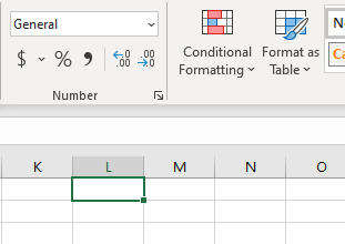
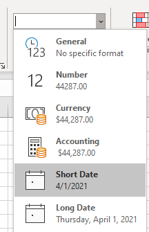
The Ribbon Home > Number menu allows you to change between Short Dates (default) and Long Dates:

Format Cells Menu – Date

The Format Cells Menu gives you numerous preset formats:

Notice that in the ‘Sample’ area you can see the impact the new number format will have on the active cell.

The Format Cells Menu can be accessed with the shortcut CTRL + 1 or by clicking this button:

Custom Number Formatting

The Custom section of the Format Cells Menu allows you the ability to create your own number formats:

To set custom number formatting for dates, you’ll need to specify how to display days, months, and / or years. Use this table as guide:

You can use the above examples to only display a day, month, or year. Or you can combine them:

Dates Stored as Text

Date as Text

To store a date as text, type an apostrophe (‘) in front of the date as you’re typing the date:

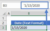
However, as long as the date is stored as text you’ll be unable to change the formatting like a normal date.

You can convert the date stored as text, back to a date using the DATEVALUE or VALUE Functions:

=DATEVALUE(B3)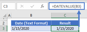

Text Function

The TEXT Function is a great way to display a date as text. The TEXT Function allows you to display dates in formats just like the Custom Number Formatting discussed previously.

=TEXT(B3,C3)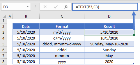

Text

You can combine the TEXT Function with a string of text like this:

="Today's date is: "&TEXT(TODAY(),"m/d/yyyy")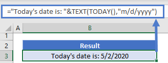

Google Sheets Date Formatting

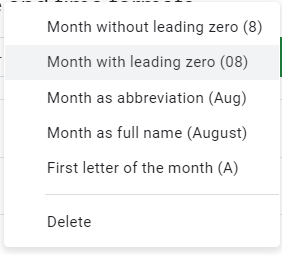
Google Sheets makes formatting dates slightly easier. With Google Sheets, you simply need to navigate to the ‘More date and time formats:

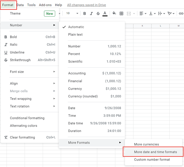
The menu looks like this:

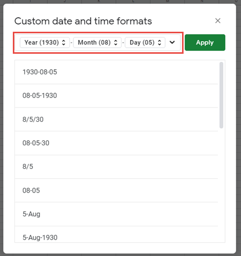
You’ll be able to select from a wide range of presets. Or you can utilize the drop-downs on top to select your desired format:

Источник

Excel Date Format (Table of Contents)

Date Format in Excel
How Excel stores Dates?
How to Change Date Format in Excel?

Date Format in Excel

A date is one of the data types that are available in excel, which we use mostly in our day to day excel data works. A date can be displayed in several ways in excel as per requirement. A date has multiple numbers of formats based on geographical regions. Because different geographical regions use a date in different ways, Excel comes with multiple numbers of formats to display dates.

How Excel Stores Dates?

Before getting into the data formats, try to understand how Excel stores dates. Excel stores the date in an integer format. To make you understand better, we will look at the following example. Consider today’s date, 11 Feb 2019.

If we observe the above date, it is in the format of Month-Day-Year. Select this date and convert this to general or number format, then we will find a number. Let’s see how to convert. Select the date and choose the drop-down list from the Number segment under the Home tab. From the drop-down, select the option General and observe how the date will be converted.

Once you convert, it will change as an integer value, as shown in the below picture.

Now we will understand what that number is and what calculation is used by Excel to convert the data into an integer. Excel gives the number series for the dates starting from 1 Jan 1900 to 31 Dec 9999, which means 1 Jan 1900 will store as 1, and 2 Jan 1900 will store as 2. Now just try to check for the date 2 Jan 1900.

When we select the general option, it converted to 2, as shown below.

I hope you understand how Excel stores the date.

How to Change Date Format in Excel?

Let’s understand how to change the date format in Excel by using some examples.

You can download this Date Format in Excel Template here – Date Format in Excel Template

Example #1

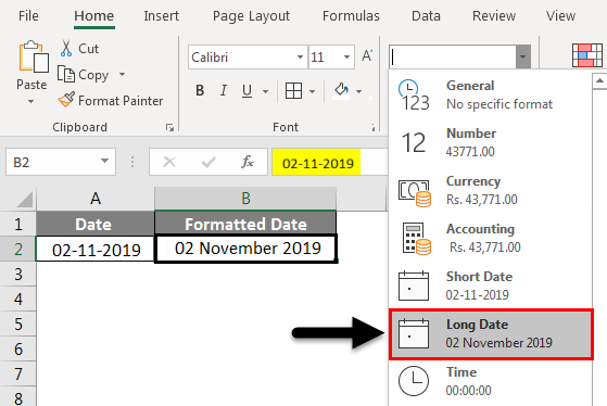
First, we will see a short date and a Long date. Then, we will find the formats Short date and Long date from the same drop list of numbers.

Short date: As the name itself speaks, how it looks like. It will display a date in a simple way that is 2/11/2019. We can observe in the drop-down itself how it will display.

Long date: It will display a date in the long format. We can observe in the below image how it will display.

Example #2

A system has one default format to display the date whenever the user inputs the date. We will see how to check the default format in excel. Then, select the date and right-click.

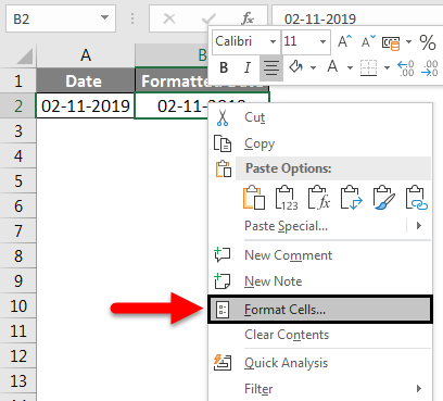
The above pop up will appear; from that pop-up menu, select the Format Cells. Then, another screen will appear, which is the “Format cells” screen in which we can apply different kinds of formats like Number, Alignment, Font, Border, fill and protection.

Select Number and select the Date from the Category box. When we select the “Date”, the right side box will show the different formats available for the different locations.

If we observe, the first two date formats, which are highlighted in the red box, have a * (asterisk) mark, which shows that those are default date formats.

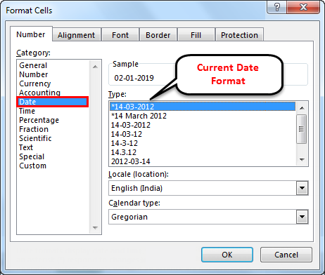
If we want to change the default date settings, we should go to the control panel and select Region and Language, then select Formats and change the date format as per your requirement.

Example #3

If we observe the below screenshot and the dates with ‘ * ‘, there are also different formats. We can select the required date format to change the current date format.

When we select the required format, we can observe a preview of how it will display in excel under the Sample box. There are different formats available like M/D, M/D/Y, MM/DD/YY etc.

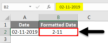
Select the M-D format, as shown below.

Then the date will look like 2-11 if we observe in the formula bar, which is highlighted. The formula bar shows as 2-11-2019; however, in Excel, it is displaying as 2-11.

We can also change the location by selecting the required location from the selected dropdown. Observe the below image how the drop-down looks like.

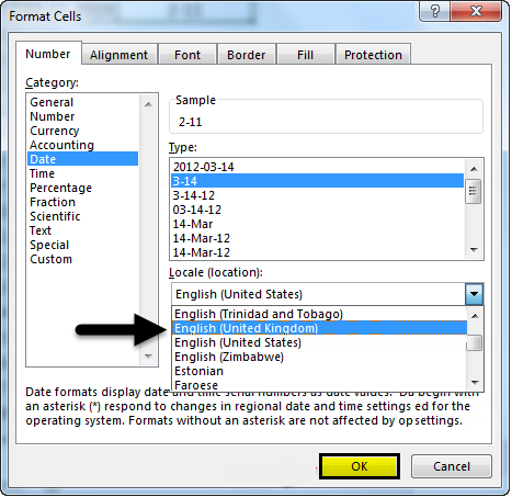
When we select a particular location from the drop-down, then different data formats will appear in the box “Type”. Currently, it is English (United States), now select the English (United Kingdom). Click OK. Then the date formats in the Type will change. Observe the below screenshot.

Observe the formats in the location United Kingdom are different from the United States. Still, if you are not happy with the date formats, we can create our customized format.

Example #4

To create a customized format, select the Custom option from the Category box.

Once we select the Custom category, we can input the required format in Type. To make it more clear, suppose we want the format like DD:MMMM: YYYY, then type this format in the “Type” box.

Observe the above image; whatever input is in Type, the same format is showing in Sample. If we click OK, then it will apply to the date in excel.

Example #5

Date format in Other languages

We can display dates in other languages too. We will be able to do this using the “custom” format under the category. For doing this, we should know that particular language code; once we know that code, we just need to add the country code before our date format.

The language code should be in square brackets preceded with $ followed by a “- “in the format of [$-xxx].

In the below example, we created the date format of the German language similarly; we can give date formats for Chinese, Spanish, Japanese, French, Italian, Greek, etc. Use Google for language codes as per your requirement.

Things to Remember

Dates before 1 Jan 1900 cannot convert to text in excel as it will not read negative numbers; hence it remains in the same format.
Dates can display in short and long formats from the drop-down number under the “Home” tab.
To convert the data into number format with the formula “Date value”.
Default date represents with “*” symbol, to change the default selection, need to go to “Control panel”.
CTRL + 1 is the shortcut for the “Format cell”. CTRL + ; is used to display the current date.

Формат даты в Excel

Прежде всего нужно чётко уяснить, как Microsoft Excel хранит дату и время. Часто это – основной источник путаницы. Хотя вы ожидаете, что он запоминает день, месяц и год, но это работает не так …

Excel хранит даты как последовательные числа, и только форматирование ячейки приводит к тому, что число отображается как дата, как время или и то, и другое вместе.

Дата в Excel

Все даты хранятся в виде целых чисел, обозначающих количество дней с 1 января 1900 г. (записывается как 1) до 31 декабря 9999 г. (сохраняется как 2958465).

В этой системе:

2 — 2 января 1900 г.
44197 — 1 января 2021 г. (потому что это 44 197 дней после 1 января 1900 г.)

Время в Excel

Время хранится в виде десятичных дробей от 0,0 до 0,99999, которые представляют собой долю дня, где 0,0 — 00:00:00, а 0,99999 — 23:59:59.

Например:

0.25 — 06:00
0.5 — 12:00.
0.541655093 это 12:59:59.

Дата и время в Excel

Дата и время хранятся в виде десятичных чисел, состоящих из целого числа, представляющего день, месяц и год, и десятичной части, представляющей время.

Например: 44197.5 — 1 января 2021 г., 12:00.

Формат даты по умолчанию в Excel и как его быстро изменить

Краткий и длинный форматы даты, которые как раз и установлены по умолчанию как основные, извлекаются из региональных настроек Windows. Они отмечены звездочкой (*) в диалоговом окне:

Они изменяются, как только вы меняете настройки даты и времени в панели управления Windows.

Если вы хотите установить другое представление даты и/или времени по умолчанию на своем компьютере, например, изменить их с американского на русское, перейдите в Панель управления и нажмите “Региональные стандарты» > «Изменение форматов даты, времени и чисел» .

На вкладке Форматы выберите регион, а затем установите желаемое отображение, щелкнув стрелку рядом с пунктом, который вы хотите изменить, и выбрав затем наиболее подходящий из раскрывающегося списка:

Если вас не устраивают варианты, предложенные на этой вкладке, нажмите кнопку “Дополнительные параметры» в нижней правой части диалогового окна. Откроется новое окно “Настройка …”, в котором вы переключаетесь на вкладку “Дата” и вводите собственный краткий или длинный формат в соответствующее поле.

Как быстро применить форматирование даты и времени по умолчанию

Как мы уже уяснили, в Microsoft Excel есть два формата даты и времени по умолчанию — короткий и длинный.

Чтобы быстро изменить один из них, сделайте следующее:

Выберите даты, которые хотите отформатировать.
На вкладке «Главная» в группе «Число» щелкните маленькую стрелку рядом с полем “Формат числа» и выберите нужный пункт — краткую дату, длинную или же время.

Если вам нужны дополнительные параметры форматирования, либо выберите “Другие числовые форматы» из раскрывающегося списка, либо нажмите кнопку запуска диалогового окна рядом с “Число».

Откроется знакомое диалоговое окно “Формат ячеек”, в котором вы сможете изменить любые нужные вам параметры. Об этом и пойдёт речь далее.

Как изменить формат даты в Excel

Даты могут отображаться разными способами. Когда дело доходит до изменения их вида для данной ячейки или диапазона, самый простой способ — открыть диалоговое окно ”Формат ячеек” и выбрать один из имеющихся там стандартных вариантов.

Выберите данные, которые вы хотите изменить, или пустые ячейки, в которые вы хотите вставить даты.
Нажмите Ctrl + 1, чтобы открыть диалоговое окно «Формат ячеек». Кроме того, вы можете кликнуть выделенные ячейки правой кнопкой мыши и выбрать этот пункт в контекстном меню.
В окне “Формат ячеек» перейдите на вкладку “Число” и выберите “Дата» в списке числовых форматов.
В разделе “Тип» выберите наиболее подходящий для вас вариант. После этого в поле “Образец» отобразится предварительный просмотр в выбранном варианте оформления.

Если вас устраивает то, что вы увидели, нажмите кнопку ОК, чтобы сохранить изменение и закрыть окно.

Если, несмотря на ваши усилия, отображение числа, месяца и года в вашей таблице не меняется, скорее всего, ваши данные записаны как текст, и вам сначала нужно преобразовать их в формат даты.

Как сменить язык даты.

Если у вас есть файл, полный иностранных дат, вы, скорее всего, захотите изменить их те, которые используются в вашей стране. Допустим, вы хотите преобразовать американский формат (месяц/день/год) в европейский стиль (день/месяц/год).

Самый простой способ сделать это заключается в следующем:

Выберите столбец, который вы хотите преобразовать в другой язык.
Используйте комбинацию Ctrl + 1, чтобы открыть знакомые нам настройки.
Выберите нужный язык в выпадающем списке «Язык (местоположение)» и нажмите «ОК», чтобы сохранить изменения.

Создание пользовательского формата даты.

Если вам не подходит ни один из стандартных вариантов, вы можете создать свой собственный.

На листе выделите нужные ячейки.
Нажмите Ctrl + 1.
На вкладке Число выберите Все форматы в списке и запишите нужный формат даты в поле Тип. Это показано на скриншоте ниже.
Щелкните ОК, чтобы сохранить изменения.

При настройке пользовательского формата даты вы можете использовать следующие коды.

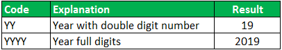
Код	Описание	Пример
м	Номер месяца без нуля в начале	1
мм	Номер месяца с нулем в начале	01
ммм	Название месяца, краткая форма	Янв
мммм	Название месяца, полная форма	Январь
ммммм	Первая буква месяца	М (обозначает март и май)
д	Номер дня без нуля в начале	1
дд	Номер дня с нулем в начале	01
ддд	День недели, краткая форма	Пн
дддд	День недели, полная форма	понедельник
гг	Год (последние 2 цифры)	05
гггг	Год (4 цифры)	2020

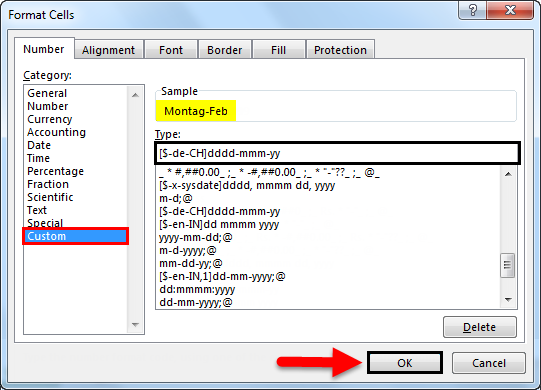
Можно также использовать дополнительные коды, которые обязательно нужно заключать в квадратные скобки [].

Код	Пояснение
x-sysdate	Системный длинный формат. Месяц в родительном падеже.
x-systime	Системное время.
x-genlower	Используется родительный падеж в нижнем регистре для любых полных названий месяцев (только для русского языка). Рекомендуется использовать вместе с кодом языка [ru-RU-x-genlower].
x-genupper	Используется родительный падеж в верхнем регистре для любых полных названий месяцев (только на русском языке). Например, [ru-RU-x-genupper].
x-nomlower	Для любых полных названий месяцев применяется именительный падеж в нижнем регистре (только на русском языке): [ru-RU-x-nomlower].

Вот как это может выглядеть на примерах:

При создании пользовательского формата в Excel вы можете использовать запятую (,), тире (-), косую черту (/), двоеточие (:) и другие символы.

Как создать собственный формат даты для другого языка

Если вы хотите отображать даты на другом языке, не меняя региональные настройки своего Windows, придётся создать собственный формат и использовать специальный префикс с соответствующим кодом языкового стандарта.

Код языка должен быть заключен в [квадратные скобки] и предваряться знаком доллара ($) и тире (-). Вот несколько примеров:

[$-419] — Россия
[$-409] – английский (США)
[$-422] — Украина
[$-423] — Беларусь
[$-407] — Германия

Вы можете найти полный список кодов языков в этом блоге.

Например, вот как это можно настроить для белорусского языка в формате времени -день-месяц-год (день недели) :

Как показать число вместо даты.

Если вы хотите узнать, какое число представляет определенную дату или время, отображаемые в ячейке, вы можете сделать это двумя способами.

1. Диалоговое окно «Форматирование ячеек»

Выделите эту ячейку, нажмите Ctrl + 1, чтобы открыть знакомое нам окно настроек и переключиться на вкладку «Общие».

Если вы просто хотите узнать число, стоящее за датой, ничего не меняя в вашей таблице, то запишите число, которое вы видите в поле «Образец», и нажмите “Отмена», чтобы закрыть окно. Если вы хотите заменить дату числом в текущей ячейке, нажмите ОК.

Вы также можете выбрать формат «Общий» на ленте в разделе «Число». Дата будет тут же заменена соответствующим ей числом.

2. Функции ДАТАЗНАЧ и ВРЕМЗНАЧ

Можно также использовать функцию ДАТАЗНАЧ(), для преобразования даты в соответствующее ей число

=ДАТАЗНАЧ(«20/1/2021»)

Используйте функцию ВРЕМЗНАЧ(), чтобы получить десятичную дробь, представляющую время

=ВРЕМЗНАЧ(«16:30»)

Чтобы узнать дату и время, объедините эти две функции следующим образом:

= ДАТАЗНАЧ(«20/1/2021») & ВРЕМЗНАЧ(«16:30»)

Получится записанное в виде текста число, соответствующее дате-времени.

А если применить операцию сложения –

= ДАТАЗНАЧ(«20/1/2021») + ВРЕМЗНАЧ(«16:30»)

То получим число, которое можно отформатировать в виде даты-времени и с которым можно производить математические операции (найти разность дат и т.п.)

Если вы запишете, скажем, 31.12.1812, то это будет текстовое значение, а не дата. Это означает, что вы не сможете выполнять обычные арифметические операции с ней. Чтобы убедиться в этом, можете ввести формулу =ДАТАЗНАЧ(«31/12/1812») в какую-нибудь ячейку, и вы получите ожидаемый результат — ошибку #ЗНАЧ!.

Формат времени в Excel

Если помните, выше мы уже говорили, что Excel обрабатывает время как часть дня, и время сохраняется как десятичная часть.

Например:

00:00:00 сохраняется как 0,0
23:59:59 сохраняется как 0,99999
06:00 — 0,25
12:00 — 0,5

Когда в ячейку вводятся и дата, и время, они сохраняются как десятичное число, состоящее из целой части, представляющего дату, и десятичной части, представляющей время.

Формат времени по умолчанию.

При изменении формата времени в диалоговом окне ”Формат ячеек” вы могли заметить, что один из пунктов начинается со звездочки (*). Это формат времени по умолчанию в вашем Excel. Как и в случае с датой, он определяется региональными настройками Windows.

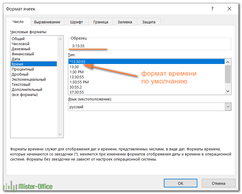
Чтобы быстро применить формат времени по умолчанию к выбранной ячейке или диапазону ячеек, щелкните стрелку раскрывающегося списка в группе Число на вкладке Главная и выберите Время.

Изменить формат времени по умолчанию, перейдите в Панель управления и перейдите “Региональные стандарты» > «Изменение форматов даты, времени и чисел». Подробно мы этот процесс описали выше, когда рассматривали установки параметров даты по умолчанию.

Десятичное представление времени.

Быстрый способ выбрать десятичное число, представляющее определенное время, — использовать диалоговое окно ”Формат ячеек”.

Просто выберите ячейку, содержащую время, и нажмите Ctrl + 1, чтобы открыть окно настроек. На вкладке “Число” выберите “Общие» в разделе “Категория», и вы увидите десятичную дробь в поле “Образец».

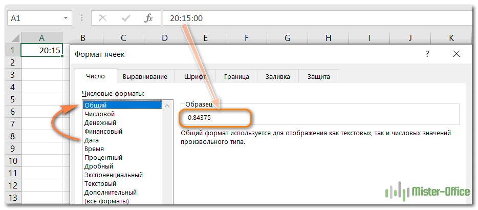
Теперь вы можете записать это число и нажать “Отмена», чтобы закрыть окно. Или же нажмите OK и замените время соответствующим десятичным числом в ячейке.

Фактически это самый быстрый, простой и не требующий формул способ преобразования времени в десятичное число.

Как применить или изменить формат времени.

Microsoft Excel достаточно умен, чтобы распознавать время при вводе и соответствующем форматировании ячейки. Например, если вы наберете 10:30 или 18:40, программа будет воспринимать и отображать это как время в зависимости от установленного по умолчанию формата времени.

Если вы хотите отформатировать некоторые числа как время или применить другой формат времени к существующим значениям, вы можете сделать это с помощью диалогового окна ”Формат ячеек”, как описано ниже.

На листе Excel выберите ячейки, в которых вы хотите применить или изменить формат времени.

2. Откройте диалоговое окно Формат ячеек , нажав Ctrl + 1или щелкнув значок “Панель запуска диалогового окна» рядом с полем ”Число» на вкладке “Главная”.

3. На вкладке “Число” выберите “Время» в списке и укажите подходящий образец в окне “Тип» .

4. Нажмите OK, чтобы применить выбранное.

Создание пользовательского формата времени.

Хотя Microsoft Excel предоставляет несколько различных форматов времени, вы можете создать свой собственный, который лучше всего подходит для конкретной задачи. Для этого откройте знакомое нам окно настроек, выберите “Все форматы» и введите подходящее время в поле “Тип» .

Созданный вами пользовательский формат времени останется в списке Тип в следующий раз, когда он вам понадобится.

Совет. Самый простой способ создать собственный формат времени – использовать один из существующих в качестве отправной точки. Для этого щелкните “Время» в списке «Категория» и выберите один из предустановленных форматов. После этого внесите в него изменения.

При этом вы можете использовать следующие коды.

Код	Описание	Отображается как
ч	Часы без нуля в начале	0:35:00
чч	Часы с нулем в начале	03:35:00
м	Минуты без нуля в начале	0:0:59
мм	Минуты с нулем в начале	00:00:59
c	Секунды без нуля в начале	00:00:9
сс	Секунды с нулем в начале	00:00:09

Когда вы рассчитываете, к примеру, табель рабочего времени, то сумма может превысить 24 часа. Чтобы Microsoft Excel правильно отображал время, выходящее за пределы суток, примените один из следующих настраиваемых форматов времени. На скриншоте ниже – отображение одного и того же времени разными способами.

Пользовательские форматы для отрицательных значений времени

Пользовательские форматы времени, описанные выше, работают только для положительных значений. Если результат ваших вычислений представляет собой отрицательное число, отформатированное как время (например, когда вы вычитаете большее количество времени из меньшего), результат будет отображаться как #####. И увеличение ширины столбца не поможет избавиться от этих решёток.

Если вы хотите обозначить отрицательные значения времени, вам доступны следующие параметры:

Отобразите пустую ячейку для отрицательных значений времени. Для этого введите точку с запятой в конце формата времени, например [ч]: мм;
Вывести сообщение об ошибке. Введите точку с запятой в конце формата времени, а затем напишите сообщение в кавычках, например

[ч]: мм; «Отрицательное время»

Если вы хотите отображать отрицательные значения времени именно как отрицательные значения, например -11:15, самый простой способ — изменить систему дат Excel на систему 1904 года. Для этого щелкните Файл> Параметры> Дополнительно, прокрутите вниз до раздела Вычисления и установите флажок Использовать систему дат 1904.

Формат «Дата – Время».

Если нужно показать и дату, и время, вы можете просто объединить в единое целое те форматы, о которых мы говорили выше.

На скриншоте ниже вы видите несколько вариантов, как могут выглядеть ваши значения:

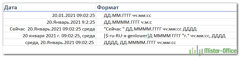
Ничего сложного: сначала описываем дату, затем – время.

Формат даты Excel не работает – как исправить?

Обычно Microsoft Excel очень хорошо понимает даты, и вы вряд ли столкнетесь с какими-либо серьёзными проблемами при работе с ними.

Но если всё же у вас возникла проблема с отображением дня, месяца и года, ознакомьтесь со следующими советами по устранению неполадок.

Ячейка недостаточно широка, чтобы вместить всю информацию.

Если вы видите на листе несколько знаков решетки (#####) вместо даты, то скорее всего, ваши ячейки недостаточно широки, чтобы вместить её целиком.

Решение. Дважды кликните по правой границе столбца, чтобы изменить его размер в соответствии с содержимым. Кроме того, вы можете просто перетащить мышкой правую границу, чтобы установить нужную ширину столбца.

Отрицательные числа форматируются как даты

Во всех современных версиях Excel 2013, 2010 и 2007 решетка (#####) также отображается, когда ячейка, отформатированная как дата или время, содержит отрицательное значение. Обычно это результат, возвращаемый какой-либо формулой. Но это также может произойти, когда вы вводите отрицательное значение в ячейку, а затем представляете эту ячейку как дату.

Если вы хотите отображать отрицательные числа как отрицательные даты, вам доступны два варианта:

Решение 1. Переключитесь на систему 1904.

Перейдите в Файл > Параметры > Дополнительно , прокрутите вниз до раздела При вычислении этой книги , установите флажок Использовать систему дат 1904 и нажмите ОК .
В этой системе 0 – это 1 января 1904 года; 1 – 2 января 1904 г .; а -1 отображается как: -2-янв-1904.
Конечно, такое представление очень необычно и требуется время, чтобы к нему привыкнуть.

Решение 2. Используйте функцию ТЕКСТ.

Другой возможный способ отображения отрицательных дат в Excel – использование функции ТЕКСТ. Например, если вы вычитаете C1 из B1, а значение в C1 больше, чем в B1, вы можете использовать следующую формулу для вывода результата в нужном вам виде:

=ТЕКСТ(ABS(B1-C1);»-ДД ММ ГГГГ»)

Получим результат «-01 01 1900».

Вы можете в формуле ТЕКСТ использовать любые другие настраиваемые форматы даты.

Замечание. В отличие от предыдущего решения, функция ТЕКСТ возвращает текстовое значение, поэтому вы не сможете использовать результат в других вычислениях.

Даты импортированы в Excel как текст

Когда вы импортируете данные из файла .csv или какой-либо другой внешней базы данных, даты часто импортируются как текстовые значения. Они могут выглядеть для вас как обычно, но Excel воспринимает их как текст и обрабатывает соответственно.

Решение. Вы можете преобразовать «текстовые даты» в надлежащий для них вид с помощью функции ДАТАЗНАЧ или функции Текст по столбцам. Подробную информацию см. в следующей статье: Как преобразовать текст в дату.

Мы рассмотрели возможные способы представления даты и времени в Excel. Спасибо за чтение!

Формат времени в Excel — Вы узнаете об особенностях формата времени Excel, как записать его в часах, минутах или секундах, как перевести в число или текст, а также о том, как добавить время с помощью…

Как сделать пользовательский числовой формат в Excel — В этом руководстве объясняются основы форматирования чисел в Excel и предоставляется подробное руководство по созданию настраиваемого пользователем формата. Вы узнаете, как отображать нужное количество десятичных знаков, изменять выравнивание или цвет шрифта,…

7 способов поменять формат ячеек в Excel — Мы рассмотрим, какие форматы данных используются в Excel. Кроме того, расскажем, как можно быстро изменять внешний вид ячеек самыми различными способами. Когда дело доходит до форматирования ячеек в Excel, большинство…

Как удалить формат ячеек в Excel — В этом коротком руководстве показано несколько быстрых способов очистки форматирования в Excel и объясняется, как удалить форматы в выбранных ячейках. Самый очевидный способ сделать часть информации более заметной — это…

8 способов разделить ячейку Excel на две или несколько — Как разделить ячейку в Excel? С помощью функции «Текст по столбцам», мгновенного заполнения, формул или вставив в нее фигуру. В этом руководстве описаны все варианты, которые помогут вам выбрать технику, наиболее подходящую…

Источник

One nice feature of Microsoft Excel is there’s usually more than one way to do many popular functions, including date formats. Whether you’ve imported data from another spreadsheet or database, or are merely entering due dates for your monthly bills, Excel can easily format most date styles.

Instructions in this article apply to Excel for Microsoft 365, Excel 2019, 2016, and 2013.

How to Change Excel Date Format Via the Format Cells Feature

With the use of Excel’s many menus, you can change up the date format within a few clicks.

Select the Home tab.
In the Cells group, select Format and choose Format Cells.
Under the Number tab in the Format Cells dialog, select Date.
As you can see, there are several options for formatting in the Type box.

You could also look through the Locale (locations) drop-down to choose a format best suited for the country you’re writing for.
Once you’ve settled on a format, select OK to change the date format of the selected cell in your Excel spreadsheet.

Make Your Own With Excel Custom Date Format

If you don’t find the format you want to use, select Custom under the Category field to format the date how you’d like. Below are some of the abbreviations you’ll need to build a customized date format.

Abbreviations used in Excel for Dates
Month shown as 1-12	m
Month shown as 01-12	mm
Month shown as Jan-Dec	mmm
Full Month Name January-December	mmmm
Month shown as the first letter of the month	mmmmm
Days (1-31)	d
Days (01-31)	dd
Days (Sun-Sat)	ddd
Days (Sunday-Saturday)	dddd
Years (00-99)	yy
Years (1900-9999)	yyyy

Select the Home tab.
Under the Cells group, select the Format drop-down, then select Format Cells.
Under the Number tab in the Format Cells dialog, select Custom. Just like the Date category, there are several formatting options.
Once you’ve settled on a format, select OK to change the date format for the selected cell in your Excel spreadsheet.

How to Format Cells Using a Mouse

If you prefer only using your mouse and want to avoid maneuvering through multiple menus, you can change the date format with the right-click context menu in Excel.

Select the cell(s) containing the dates you want to change the format of.
Right-click the selection and select Format Cells. Alternatively, press Ctrl+1 to open the Format Cells dialog.

Alternatively, select Home > Number, select the arrow, then select Number Format at the bottom right of the group. Or, in the Number group, you can select the drop-down box, then select More Number Formats.
Select Date, or, if you need a more customized format, select Custom.
In the Type field, select the option that best suits your formatting needs. This might take a bit of trial and error to get the right formatting.
Select OK when you’ve chosen your date format.

Whether using the Date or Custom category, if you see one of the Types with an asterisk (*) this format will change depending on the locale (location) you have selected.

Using Quick Apply for Long or Short Date

If you need a quick format change from to either a Short Date (mm/dd/yyyy) or Long Date (dddd, mmmm dd, yyyy or Monday, January 1, 2019), there’s a quick way to change this in the Excel Ribbon.

Select the cell(s) for which you want to change the date format.
Select Home.
In the Number group, select the drop-down menu, then select either Short Date or Long Date.

Using the TEXT Formula to Format Dates

This formula is an excellent choice if you need to keep your original date cells intact. Using TEXT, you can dictate the format in other cells in any foreseeable format.

To get started with the TEXT formula, go to a different cell, then enter the following to change the format:

=TEXT(##, “format abbreviations”)

## is the cell label, and format abbreviations are the ones listed above under the Custom section. For example, =TEXT(A2, “mm/dd/yyyy”) displays as 01/01/1900.

Using Find & Replace to Format Dates

This method is best used if you need to change the format from dashes (-), slashes (/), or periods (.) to separate the month, day, and year. This is especially handy if you need to change a large number of dates.

Select the cell(s) you need to change the date format for.
Select Home > Find & Select > Replace.
In the Find what field, enter your original date separator (dash, slash, or period).
In the Replace with field, enter what you’d like to change the format separator to (dash, slash, or period).
Then select one of the following:
- Replace All: Which will replace all the first field entry and replace it with your choice from the Replace with field.
- Replace: Replaces the first instance only.
- Find All: Only finds all of the original entry in the Find what field.
- Find Next: Only finds the next instance from your entry in the Find what field.

Using Text to Columns to Convert to Date Format

If you have your dates formatted as a string of numbers and the cell format is set to text, Text to Columns can help you convert that string of numbers into a more recognizable date format.

Select the cell(s) that you want to change the date format.
Make sure they are formatted as Text. (Press Ctrl+1 to check their format).
Select the Data tab.
In the Data Tools group, select Text to Columns.
Select either Delimited or Fixed width, then select Next.

Most of the time, Delimited should be selected, as date length can fluctuate.
Uncheck all of the Delimiters and select Next.
Under the Column data format area, select Date, choose the format your date string using the drop-down menu, then select Finish.

Using Error Checking to Change Date Format

If you’ve imported dates from another file source or have entered two-digit years into cells formatted as Text, you’ll notice the small green triangle in the top-left corner of the cell.

This is Excel’s Error Checking indicating an issue. Because of a setting in Error Checking, Excel will identify a possible issue with two-digit year formats. To use Error Checking to change your date format, do the following:

Select one of the cells containing the indicator. You should notice an exclamation mark with a drop-down menu next to it.
Select the drop-down menu and select either Convert XX to 19XX or Convert xx to 20XX, depending on the year it should be.
You should see the date immediately change to a four-digit number.

Using Quick Analysis to Access Format Cells

Quick Analysis can be used for more than formatting the color and style of your cells. You can also use it to access the Format Cells dialog.

Select several cells containing the dates you need to change.
Select Quick Analysis in the lower right of your selection, or press Ctrl+Q.
Under Formatting, select Text That Contains.
Using the right drop-down menu, select Custom Format.
Select the Number tab, then select either Date or Custom.
Select OK twice when complete.

Thanks for letting us know!

Get the Latest Tech News Delivered Every Day

Источник

In this article

Display numbers as dates or times

Create a custom date or time format

Tips for displaying dates or times

Need more help?

Need more help?

Want more options?

Step 1. Select the range of cells containing the date

Step 2. Go to Number Format dropdown

Step 3. Choose Date

Choose the Date Type

Choose the Locale (location)

Choose the type of calendar

Conclusion

What is a date in Excel?

Dates are whole numbers

Explanation of the numbering

Date format

How to customize a date?

Don’t write text in your cell !!!

Different examples of custom date

Different writing of dates according to the format code

What is the Date Format in Excel?

Table of contents

Code of Date Format in Excel

How to Change Date Format in Excel?

Example #1–Apply Default Format of Long Date in Excel

Example #2–Change the Date Excel Format Using “Custom” Option

Example #3–Apply Different Types of Customized Date Formats in Excel

Example #4–Convert Text Values Representing Dates to Actual Dates

Example #5–Change the Date Format Using “Find and Replace” Box

Frequently Asked Questions

Recommended Articles

Choosing from the Date Format List

How to Change The Excel Date Format

Creating a Custom Excel Date Format Option

Converting Date Formats to Other Locales

Tips for Displaying Dates in Excel

Why Your Date Format May Not Be Having Issues Changing

Data Preparation with Excel

Excel Date Format

Change Date Formats

Short Date / Long Date

Format Cells Menu – Date

Custom Number Formatting

Dates Stored as Text

Date as Text

Text Function

Google Sheets Date Formatting

Date Format in Excel

How Excel Stores Dates?

How to Change Date Format in Excel?

Example #1

Example #2

Example #3

Example #4

Example #5

Things to Remember

Recommended Articles

Формат даты в Excel

Дата в Excel

Время в Excel

Дата и время в Excel

Формат даты по умолчанию в Excel и как его быстро изменить

Как быстро применить форматирование даты и времени по умолчанию

Как изменить формат даты в Excel

Как сменить язык даты.

Создание пользовательского формата даты.

Как создать собственный формат даты для другого языка

Как показать число вместо даты.

1. Диалоговое окно «Форматирование ячеек»

2. Функции ДАТАЗНАЧ и ВРЕМЗНАЧ

Формат времени в Excel

Формат времени по умолчанию.

Десятичное представление времени.

Как применить или изменить формат времени.

Создание пользовательского формата времени.

Пользовательские форматы для отрицательных значений времени

Формат «Дата – Время».

Формат даты Excel не работает – как исправить?