

I want to cover something today that I use all of the time but seems to be understood in varying degrees by clients I work with.
I am talking about use of the dollar sign ($) in an Excel formula.
Relative cell references
When you copy and paste an Excel formula from one cell to another, the cell references change, relative to the new position:
EXAMPLE:
If we have the very simple formula «=A1» in cell B1 it will change as follows when copied and pasted:
Pasted to B2, it becomes «=A2»
Pasted to C2, it becomes «=B2»
Pasted to A2, it returns an error!
In each case it is changing the reference to refer to the cell one to the left on the same row as the cell that the formula is in, i.e. the same relative position that A1 was to the original formula.
The reason an error is returned when it is pasted into column A, is because there are no columns to the left of column A.
This behaviour is very useful and is what allows a sum to be copied across or down the page and automatically refer to the new column or row that it finds itself in.
But in some situations, you want some or all of the references to remain fixed when they are copied elsewhere.
The dollar sign ($)
This is where the dollar sign is used.
EXAMPLE:
Take an example where you have a column of Sales values in Pounds Sterling in column A and a formula to convert these into US Dollars in column B. You could enter the actual exchange rate into the formula but it would be more sensible to refer to a cell where the exchange rate is held, so that it can be updated whenever it is needed.
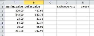
The simple formula for cell B2, would be «=A2*E1», however if you copy this down, then the formula in cell B3, would read «=A3*E2» as both references would move down a row as described above.
This is where the dollar sign ($) is used. The dollar sign allows you to fix either the row, the column or both on any cell reference, by preceding the column or row with the dollar sign. In our example if we replace the formula in cell B2 with «=A2*$E$1», then both the «E» and the «1» will remain fixed when the formula is copied. i.e. in cell B3, the formula will read «=A3*$E$1», still referring to the cell with the exchange rate in it.
In this example we have fixed both the row and the column, but in other situations, you may just want to fix one or the other, for example:

Above we have a spreadsheet calculating the times tables where we want to every cell in the white area to be the product of its row and column heading. This is easy using the dollar symbol. In cell B2, the formula without dollars would be «=A2*B1», but for this formula to work when copied to each column, we need it to always look at column A for the first reference and to work for each row, we need to always look at row 1 for the second. Using the dollar sign to do this, it becomes «=$A2*B$1». This can then be copied to every cell in the white area.
Quick Tip
You can speed up entering the dollar signs by using the function key F4 when editing the formula, if the cursor is on a cell reference in the formula, repeatedly hitting the F4 key, toggles between no dollar signs, both dollar signs, just the row and just the column.
If you enjoyed this post, go to the top of the blog, where you can subscribe for regular updates and get your free report «The 5 Excel features that you NEED to know».
Select the column that’s immediately to the right of the last column you want frozen. Select the View tab, Windows Group, click the Freeze Panes drop down and select Freeze Panes. Excel inserts a thin line to show you where the frozen pane begins.
Contents
- 1 How do you keep a cell fixed in Excel?
- 2 How do I fix a cell in Excel without F4?
- 3 What is the F4 key on Mac for Excel?
- 4 What is the F5 key?
- 5 What can I use instead of F4?
- 6 What is Alt and F4?
- 7 How do I fix #value in Excel?
- 8 How do I type F4 in Excel?
- 9 How do you fix cells in Excel for Mac?
- 10 Why is F4 not repeating in Excel?
- 11 What is F8 in Excel?
- 12 What does the F11 key do?
- 13 What is F9 used for in Excel?
- 14 What does F5 key do in Excel?
- 15 How do I use F4 without FN?
- 16 Why is F4 not working?
- 17 What is Ctrl N?
- 18 What Ctrl Z do?
- 19 What is Ctrl Shift QQ?
- 20 What is fixing in Excel?
How do you keep a cell fixed in Excel?
There is a shortcut for placing absolute cell references in your formulas! When you are typing your formula, after you type a cell reference – press the F4 key. Excel automatically makes the cell reference absolute!
How do I fix a cell in Excel without F4?
The problem isn’t in Excel, it’s in the computer BIOS settings. The function keys are not in function mode, but are in multimedia mode by default! You can change this so that you don’t have to press the combination of Fn+F4 each time you want to lock the cell.
What is the F4 key on Mac for Excel?
The shortcut to toggle absolute and relative references is F4 in Windows, while on a Mac, its Command T. For a complete list of Windows and Mac shortcuts, see our side-by-side list. If you want to see more Excel shortcuts for the Mac in action, see our our video tips.
What is the F5 key?
F5. In all modern Internet browsers, pressing F5 will reload or refresh the document window or page. Ctrl+F5 forces a complete refresh of a web page. It clears the cache and downloads all contents of the page again.
What can I use instead of F4?
The F4 shortcut to lock a reference only works on Windows. If you’re running MAC, use the shortcut: ⌘ + T to toggle absolute and relative references. You can’t select a cell and press F4 and have it change all references to absolute.
What is Alt and F4?
Alt + F4 is a Windows keyboard shortcut that completely closes the application you’re using. It differs slightly from Ctrl + F4, which closes the current window of the application you’re viewing.
How do I fix #value in Excel?
Remove spaces that cause #VALUE!
- Select referenced cells. Find cells that your formula is referencing and select them.
- Find and replace.
- Replace spaces with nothing.
- Replace or Replace all.
- Turn on the filter.
- Set the filter.
- Select any unnamed checkboxes.
- Select blank cells, and delete.
How do I type F4 in Excel?
How to use F4 in Excel. Using the F4 key in Excel is quite easy. Think of a situation where you have been working on an Excel worksheet and you want to repeat the last action multiple times. All you need to do is press and hold Fn and then press and release the F4 key.
How do you fix cells in Excel for Mac?
Freeze panes to lock the first row or column in Excel for Mac
- Freeze the top row. On the View tab, click Freeze Top Row.
- Freeze the first column. If you’d rather freeze the leftmost column instead, on the View tab, click Freeze First Column.
- Freeze as many rows or columns as you want.
Why is F4 not repeating in Excel?
For troubleshooting, you may try to open Excel application in safe mode and check if F4 works. If it works, the issue should be caused by Excel add-ins. Besides, try to Online Repair Office and see if issue can be fixed.
What is F8 in Excel?
F8 Turns extend mode on or off. In extend mode, Extended Selection appears in the status line, and the arrow keys extend the selection. Shift+F8 enables you to add a nonadjacent cell or range to a selection of cells by using the arrow keys.
What does the F11 key do?
The F11 key allows you to activate full-screen mode in your browser. By pressing it again, you will return to the standard view with the menu bar. In Microsoft Excel, you can use the Shift key with F11 to quickly create a new spreadsheet in a new tab.
What is F9 used for in Excel?
Shortcut keys in Excel – Function Keys (6 of 
| Key | Description |
|---|---|
| Ctrl+F8: Performs the Size command when a workbook is not maximized. | |
| Alt+F8: Displays the Macro dialog box to create, run, edit, or delete a macro. | |
| F9 | F9: Calculates all worksheets in all open workbooks. |
| Shift+F9: Calculates the active worksheet. |
What does F5 key do in Excel?
F5. Displays the Go To dialog box. For example, to select cell C15, in the Reference box, type C15, and click OK. Note: you can also select named ranges, or click Special to quickly select all cells with formulas, comments, conditional formatting, constants, data validation, etc.
How do I use F4 without FN?
All you have to do is look on your keyboard and search for any key with a padlock symbol on it. Once you’ve located this key, press the Fn key and the Fn Lock key at the same time. Now, you’ll be able to use your Fn keys without having to press the Fn key to perform functions.
Why is F4 not working?
If the Alt + F4 combo fails to do what it is supposed to do, then press the Fn key and try the Alt + F4 shortcut again. Still not working? Try pressing Fn + F4. If you still cannot notice any change, try holding down Fn for a few seconds.
What is Ctrl N?
Alternatively referred to as Control+N and C-n, Ctrl+N is a keyboard shortcut most often used to create a new document, window, workbook, or other type of file.Ctrl+N in Word and other word processors.
What Ctrl Z do?
To reverse your last action, press CTRL+Z. You can reverse more than one action. To reverse your last Undo, press CTRL+Y. You can reverse more than one action that has been undone.
What is Ctrl Shift QQ?
Ctrl-Shift-Q, if you aren’t familiar, is a native Chrome shortcut that closes every tab and window you have open without warning.
What is fixing in Excel?
The Microsoft Excel FIX function returns the integer portion of a number. The FIX function is a built-in function in Excel that is categorized as a Math/Trig Function. It can be used as a VBA function (VBA) in Excel.
Содержание
- Fix data that is cut off in cells
- Wrap text in a cell
- Start a new line in the cell
- Reduce the font size to fit data in the cell
- Reposition the contents of the cell by changing alignment or rotating text
- Change the font size
- How To Fix Cell In Excel?
- How do you keep a cell fixed in Excel?
- How do I fix a cell in Excel without F4?
- What is the F4 key on Mac for Excel?
- What is the F5 key?
- What can I use instead of F4?
- What is Alt and F4?
- How do I fix #value in Excel?
- How do I type F4 in Excel?
- How do you fix cells in Excel for Mac?
- Why is F4 not repeating in Excel?
- What is F8 in Excel?
- What does the F11 key do?
- What is F9 used for in Excel?
- What does F5 key do in Excel?
- How do I use F4 without FN?
- Why is F4 not working?
- What is Ctrl N?
- What Ctrl Z do?
- What is Ctrl Shift QQ?
- What is fixing in Excel?
- Absolute link in Excel fixes the cell in the formula
- Absolute and relative links in Excel
- Use of absolute and relative links in Excel
Fix data that is cut off in cells
Wrap text, change the alignment, decrease the font size, or rotate your text so that everything you want fits inside a cell.
Wrap text in a cell
You can format a cell so that text wraps automatically.
Select the cells.
On the Home tab, click Wrap Text.
The text in the selected cell wraps to fit the column width. When you change the column width, text wrapping adjusts automatically.
Note: If all wrapped text is not visible, it might be because the row is set to a specific height. To enable the row to adjust automatically and show all wrapped text, on the Format menu, point to Row, and then click AutoFit.
Start a new line in the cell
Inserting a line break may make text in a cell easier to read.
Double-click in the cell.
Click where you want to insert a line break, and then press CONTROL + OPTION + RETURN .
Reduce the font size to fit data in the cell
Excel can reduce the font size to show all data in a cell. If you enter more content into the cell, Excel will continue to reduce the font size.
Select the cells.
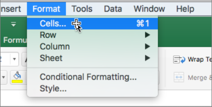
Right-click and select Format Cells.
In the Format Cells dialog box, select the checkbox next to Shrink to fit.
Data in the cell reduces to fit the column width. When you change the column width or enter more data, the font size adjusts automatically.
Reposition the contents of the cell by changing alignment or rotating text
For the optimal display of the data on your sheet, you may want to reposition the text in a cell. You can change the alignment of the cell contents, use indentation for better spacing, or display the data at a different angle by rotating it.
Select the cell or range of cells that contains the data that you want to reposition.
On the Format menu, click Cells.
In the Format Cells box, and in the Alignment tab, do any of the following:
Change the horizontal alignment of the cell contents
On the Horizontal pop-up menu, click the alignment that you want.
If you select the Fill option or Center Across Selection option, text rotation will not be available for those cells.
Change the vertical alignment of the cell contents
On the Vertical pop-up menu, click the alignment that you want.
Indent the cell contents
On the Horizontal pop-up menu, click Left (Indent), Right, or Distributed, and then type the amount of indentation (in characters) that you want in the Indent box.
Display the cell contents vertically from top to bottom
Under Orientation, click the box that contains the vertical text.
Rotate the text in a cell
Under Orientation, click or drag the indicator to the angle that you want, or type an angle in the Degrees box.
Restore the default alignment of selected cells
On the Horizontal pop-up menu, click General.
Note: If you save the workbook in another file format, text that was rotated may not display at the correct angle. Most file formats do not support rotation within the full 180 degrees (+90 through –90 degrees) that is possible in the latest versions of Excel. For example, earlier versions of Excel can rotate text only at angles of +90, 0 (zero), or –90 degrees.
Change the font size
Select the cells.
On the Home tab, in the Font size box, enter a different number, or click to reduce the font size.
Источник
How To Fix Cell In Excel?
Select the column that’s immediately to the right of the last column you want frozen. Select the View tab, Windows Group, click the Freeze Panes drop down and select Freeze Panes. Excel inserts a thin line to show you where the frozen pane begins.
How do you keep a cell fixed in Excel?
There is a shortcut for placing absolute cell references in your formulas! When you are typing your formula, after you type a cell reference – press the F4 key. Excel automatically makes the cell reference absolute!
How do I fix a cell in Excel without F4?
The problem isn’t in Excel, it’s in the computer BIOS settings. The function keys are not in function mode, but are in multimedia mode by default! You can change this so that you don’t have to press the combination of Fn+F4 each time you want to lock the cell.
What is the F4 key on Mac for Excel?
The shortcut to toggle absolute and relative references is F4 in Windows, while on a Mac, its Command T. For a complete list of Windows and Mac shortcuts, see our side-by-side list. If you want to see more Excel shortcuts for the Mac in action, see our our video tips.
What is the F5 key?
F5. In all modern Internet browsers, pressing F5 will reload or refresh the document window or page. Ctrl+F5 forces a complete refresh of a web page. It clears the cache and downloads all contents of the page again.
What can I use instead of F4?
The F4 shortcut to lock a reference only works on Windows. If you’re running MAC, use the shortcut: ⌘ + T to toggle absolute and relative references. You can’t select a cell and press F4 and have it change all references to absolute.
What is Alt and F4?
Alt + F4 is a Windows keyboard shortcut that completely closes the application you’re using. It differs slightly from Ctrl + F4, which closes the current window of the application you’re viewing.
How do I fix #value in Excel?
Remove spaces that cause #VALUE!
- Select referenced cells. Find cells that your formula is referencing and select them.
- Find and replace.
- Replace spaces with nothing.
- Replace or Replace all.
- Turn on the filter.
- Set the filter.
- Select any unnamed checkboxes.
- Select blank cells, and delete.
How do I type F4 in Excel?
How to use F4 in Excel. Using the F4 key in Excel is quite easy. Think of a situation where you have been working on an Excel worksheet and you want to repeat the last action multiple times. All you need to do is press and hold Fn and then press and release the F4 key.
How do you fix cells in Excel for Mac?
Freeze panes to lock the first row or column in Excel for Mac
- Freeze the top row. On the View tab, click Freeze Top Row.
- Freeze the first column. If you’d rather freeze the leftmost column instead, on the View tab, click Freeze First Column.
- Freeze as many rows or columns as you want.
Why is F4 not repeating in Excel?
For troubleshooting, you may try to open Excel application in safe mode and check if F4 works. If it works, the issue should be caused by Excel add-ins. Besides, try to Online Repair Office and see if issue can be fixed.
What is F8 in Excel?
F8 Turns extend mode on or off. In extend mode, Extended Selection appears in the status line, and the arrow keys extend the selection. Shift+F8 enables you to add a nonadjacent cell or range to a selection of cells by using the arrow keys.
What does the F11 key do?
The F11 key allows you to activate full-screen mode in your browser. By pressing it again, you will return to the standard view with the menu bar. In Microsoft Excel, you can use the Shift key with F11 to quickly create a new spreadsheet in a new tab.
What is F9 used for in Excel?
Shortcut keys in Excel – Function Keys (6 of
| Key | Description |
|---|---|
| Ctrl+F8: Performs the Size command when a workbook is not maximized. | |
| Alt+F8: Displays the Macro dialog box to create, run, edit, or delete a macro. | |
| F9 | F9: Calculates all worksheets in all open workbooks. |
| Shift+F9: Calculates the active worksheet. |
What does F5 key do in Excel?
F5. Displays the Go To dialog box. For example, to select cell C15, in the Reference box, type C15, and click OK. Note: you can also select named ranges, or click Special to quickly select all cells with formulas, comments, conditional formatting, constants, data validation, etc.
How do I use F4 without FN?
All you have to do is look on your keyboard and search for any key with a padlock symbol on it. Once you’ve located this key, press the Fn key and the Fn Lock key at the same time. Now, you’ll be able to use your Fn keys without having to press the Fn key to perform functions.
Why is F4 not working?
If the Alt + F4 combo fails to do what it is supposed to do, then press the Fn key and try the Alt + F4 shortcut again. Still not working? Try pressing Fn + F4. If you still cannot notice any change, try holding down Fn for a few seconds.
What is Ctrl N?
Alternatively referred to as Control+N and C-n, Ctrl+N is a keyboard shortcut most often used to create a new document, window, workbook, or other type of file.Ctrl+N in Word and other word processors.
What Ctrl Z do?
To reverse your last action, press CTRL+Z. You can reverse more than one action. To reverse your last Undo, press CTRL+Y. You can reverse more than one action that has been undone.
What is Ctrl Shift QQ?
Ctrl-Shift-Q, if you aren’t familiar, is a native Chrome shortcut that closes every tab and window you have open without warning.
What is fixing in Excel?
The Microsoft Excel FIX function returns the integer portion of a number. The FIX function is a built-in function in Excel that is categorized as a Math/Trig Function. It can be used as a VBA function (VBA) in Excel.
Источник
Absolute link in Excel fixes the cell in the formula
The advantages of absolute references are difficult to underestimate. They often have to be used in the process of working with the program. Relative references to cells in Excel are more popular than absolute ones, but they also have their pros and cons.
In Excel, there are several types of links: absolute, relative and mixed. This also includes «names» for whole ranges of cells. Consider their possibilities and differences in practical application in formulas.
Absolute and relative links in Excel
Absolute references allow us to fix a row or column (or row and column at a time) to which the formula should refer. Relative references in Excel change automatically when you copy a formula along a range of cells, both vertically and horizontally. A simple example of relative cell addresses. Let us calculate the volume of the sphere in Excel:

- Fill the range of cells A2: A5 with different radii.
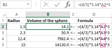
- In cell B2, enter the formula for calculating the volume of the sphere, which will refer to the value of A2. The formula will look like this: =(4/3)*3.14*A2^3
- Copy the formula from B2 along column A2: A5.
As you can see, the relative addresses help to change the address in each formula automatically.
It is also worth to point the regularity of changes in references of formulas. Data in B3 refers to A3, B4 to A4, and so on. Everything depends on where the first introduced formula will refer, and its copies will change the references relative to its position in the range of cells on the sheet.
Now instead of numbers we use absolute references:
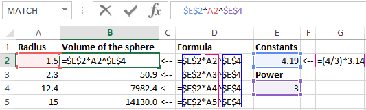
The result of the calculation is the same, but the formulas are more flexible to the changes. It is enough to change the value in one cell and the whole column is recalculated automatically. See the following example.
Use of absolute and relative links in Excel
Fill in the plate, as shown in the picture:
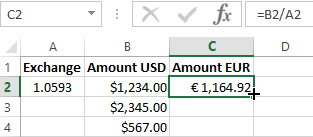
Description of the source table. In cell A2, there is an actual euro exchange rate against the dollar for today. In the range of cells B2: B4 are the amounts in dollars. In the range C2: C4 will be the amount in euros after the conversion of currencies. Tomorrow the course will change and the task of the plate will automatically recalculate the range of C2: C4 depending on the change in the value in cell A2 (that is, the euro rate).
To solve this problem, we need to enter a formula in C2: = B2 / A2 and copy it to all cells in the C2: C4 range. But here there is a problem. From the previous example, we know that when copying, relative references automatically change addresses relative to their position. Therefore, an error occurs:
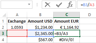
Concerning the first argument, this is quite acceptable. After all, the formula automatically refers to the new value in the column of the table cells (dollar amounts). But the second indicator we need to fix on the address A2. Accordingly, it is necessary to change the relative reference to the absolute in the formula.
How to make an absolute reference in Excel? It is very simple to put the $ (dollar) symbol before the line or column number or before the both of them. Below, consider all 3 options and determine their differences.
Our new formula should contain at once 2 types of links: absolute and relative.
- In C2, enter another formula: = B2 / A $ 2. To change links in Excel, double click on the cell with the left mouse button or press the F2 key on the keyboard.
- Copy it to the other cells in the C3:C4 range.
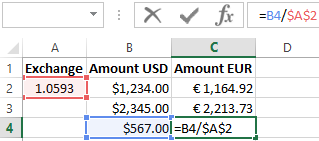
Description of the new formula. The dollar symbol ($) in the address of references fixes the address in the new copied formulas.
Absolute, relative and mixed references in Excel:
- $ A $ 2 — address of the absolute reference with fixation on columns and rows, both vertically and horizontally.
- $ A2 is a mixed link. When copying a column is fixed, and the row is changed.
- A $ 2 is a mixed link. When copying a row is fixed, and the column is changed.
For comparison: A2 is a relative address, without fixation. During the copying of the formulas, the row (2) and the column (A) automatically change to the new addresses relative to the location of the copied formula, both vertically and horizontally.
Note. In this example, the formula can contain not only a mixed link, but the absolute result: = B2 / $ A $ 2. The result will be the same. But in practice, there are often cases when you cannot do a thing without mixed references.
Helpful advice. To avoid entering the dollar symbol ($) manually, after specifying the address, press F4 repeatedly to select the required type: absolute or mixed. It’s fast and convenient.
Источник
The advantages of absolute references are difficult to underestimate. They often have to be used in the process of working with the program. Relative references to cells in Excel are more popular than absolute ones, but they also have their pros and cons.
In Excel, there are several types of links: absolute, relative and mixed. This also includes «names» for whole ranges of cells. Consider their possibilities and differences in practical application in formulas.
Absolute and relative links in Excel
Absolute references allow us to fix a row or column (or row and column at a time) to which the formula should refer. Relative references in Excel change automatically when you copy a formula along a range of cells, both vertically and horizontally. A simple example of relative cell addresses. Let us calculate the volume of the sphere in Excel:
- Fill the range of cells A2: A5 with different radii.
- In cell B2, enter the formula for calculating the volume of the sphere, which will refer to the value of A2. The formula will look like this: =(4/3)*3.14*A2^3
- Copy the formula from B2 along column A2: A5.
As you can see, the relative addresses help to change the address in each formula automatically.
It is also worth to point the regularity of changes in references of formulas. Data in B3 refers to A3, B4 to A4, and so on. Everything depends on where the first introduced formula will refer, and its copies will change the references relative to its position in the range of cells on the sheet.
Now instead of numbers we use absolute references:
The result of the calculation is the same, but the formulas are more flexible to the changes. It is enough to change the value in one cell and the whole column is recalculated automatically. See the following example.
Use of absolute and relative links in Excel
Fill in the plate, as shown in the picture:
Description of the source table. In cell A2, there is an actual euro exchange rate against the dollar for today. In the range of cells B2: B4 are the amounts in dollars. In the range C2: C4 will be the amount in euros after the conversion of currencies. Tomorrow the course will change and the task of the plate will automatically recalculate the range of C2: C4 depending on the change in the value in cell A2 (that is, the euro rate).
To solve this problem, we need to enter a formula in C2: = B2 / A2 and copy it to all cells in the C2: C4 range. But here there is a problem. From the previous example, we know that when copying, relative references automatically change addresses relative to their position. Therefore, an error occurs:
Concerning the first argument, this is quite acceptable. After all, the formula automatically refers to the new value in the column of the table cells (dollar amounts). But the second indicator we need to fix on the address A2. Accordingly, it is necessary to change the relative reference to the absolute in the formula.
How to make an absolute reference in Excel? It is very simple to put the $ (dollar) symbol before the line or column number or before the both of them. Below, consider all 3 options and determine their differences.
Our new formula should contain at once 2 types of links: absolute and relative.
- In C2, enter another formula: = B2 / A $ 2. To change links in Excel, double click on the cell with the left mouse button or press the F2 key on the keyboard.
- Copy it to the other cells in the C3:C4 range.
Description of the new formula. The dollar symbol ($) in the address of references fixes the address in the new copied formulas.
Absolute, relative and mixed references in Excel:
- $ A $ 2 — address of the absolute reference with fixation on columns and rows, both vertically and horizontally.
- $ A2 is a mixed link. When copying a column is fixed, and the row is changed.
- A $ 2 is a mixed link. When copying a row is fixed, and the column is changed.
For comparison: A2 is a relative address, without fixation. During the copying of the formulas, the row (2) and the column (A) automatically change to the new addresses relative to the location of the copied formula, both vertically and horizontally.
Note. In this example, the formula can contain not only a mixed link, but the absolute result: = B2 / $ A $ 2. The result will be the same. But in practice, there are often cases when you cannot do a thing without mixed references.
Helpful advice. To avoid entering the dollar symbol ($) manually, after specifying the address, press F4 repeatedly to select the required type: absolute or mixed. It’s fast and convenient.
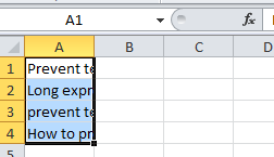
Are you annoyed with adjusting data in Excel cells? Trying hard to prevent Excel cells from spilling over or Excel cells overlapping?
Not to worry…! This blog will help you out to fix Excel cells overlapping issues easily and instantly.
Just go through all the fixes mentioned in this post.
Take a quick precape over the Excel Cells Overlapping fixes.
- Use Format Cells Option
- Autofit Columns And Rows
- Manually Resize The Cell
- Prevent Excel Cells From Spilling Over With Wrap Text
- With The Justify Feature
By following all these fixes you can easily fix Excel cells from spilling over:
To extract data from corrupt Excel file, we recommend this tool:
This software will prevent Excel workbook data such as BI data, financial reports & other analytical information from corruption and data loss. With this software you can rebuild corrupt Excel files and restore every single visual representation & dataset to its original, intact state in 3 easy steps:
- Download Excel File Repair Tool rated Excellent by Softpedia, Softonic & CNET.
- Select the corrupt Excel file (XLS, XLSX) & click Repair to initiate the repair process.
- Preview the repaired files and click Save File to save the files at desired location.
1# Use Format Cells Option
To prevent Excel cells overlapping the very first solution you need to use is the format cell option.
- Choose the excel cells in which you want to fix Excel cells overlapping issues.
- Now from the context menu choose the Format Cells.
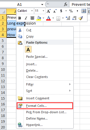
- In the opened dialog box of Format Cells, hit the Alignment Here you will see a horizontal option from its drop-down list choose the Fill.

- Tap the OK button. After that, you will see that the data present within the selected cells won’t spill over.
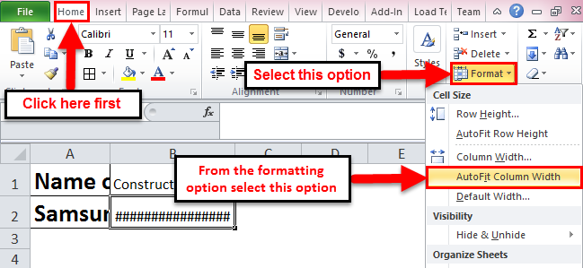
2# Autofit Columns And Rows
You can auto-fit the column and rows of your Excel worksheets to prevent Excel cells from spilling over.
One way is by making double tap on the rows and column border
Place your mouse pointer on the right border of your column heading unless and until you see a double-headed arrow. After then make a double-tap on the border.
Another way is by using the AutoFit option of columns and rows from the ribbon.
To Autofit The Column Width:
- Choose one or all columns of your worksheet. Now tap to the Home tab from the Excel ribbon.
- From the cells group, you have to hit the Format> AutoFit Column Width option.
To Autofit The Row Height:
- Choose the row in which you are facing such Excel cells overlapping
- Now tap to the Home tab from the Excel ribbon.
- From the cells group you have to hit the Format> AutoFit Row Height option.

3# Manually Resize The Cell
If your cells text are overlapping and thus you want to increase the white space around your cells. For this, you need to resize your cells by using the AutoFit option.
- At first, you need to go to the home> Format Now from the drop-down menu of Format option choose the “Column Width”.
- In the column, the width field assigns the width size in pixel and then click OK.

If you are facing difficulty to assign correct measurement then resize the cell using the dragging technique.
Put your mouse pointer on the column border and then drag the border on the right side for increasing up the column width.
4# Prevent Excel Cells From Spilling Over With Wrap Text
Does your Excel column with the long comments spill over the adjacent cells, in that case, try the following fixes?
In the figure you can see, long comments or text of B columns spills over the C columns when it is blank.

To fix this issue, you need to turn on the wrap text option for column B.
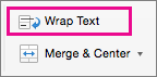
- Tap to the home Now from the alignment group you have to hit the Wrap text option.

Doing this will make your row quite taller in size for adjusting your long comment.
- After that hit the Home> Format> Row Height In the opened window you have to assign the value 12.75.

- This will show all your cell text in normal height rows without spilling it over the adjacent blank cells.

5# Use The Justify Feature
For preventing text from extending beyond your Excel report width you can use the justify feature.
Let’s now how it is to be done with an example:
- Make sure your typed text is only kept in cell A2.
- Now choose the cell A2:D2.
- In the Excel menu bar, go to the Home Now from the “Editing” group, click the “Fill” option drop-down button. From the drop-down list choose the “Justify” option.

- After hitting the justify option you will get the following message: Text will extend the below-selected range.

Note: Before clicking this OK option, make sure that the below cells are empty.

Another method for this:
- From your keyboard press the Ctrl+1 button. This will open the dialog box of Format cells on your screen.

- Now go to the Alignment tab and from the vertical section, the drop-down list hit the Justify option. After that tap the OK button.

In this way, you can easily prevent Excel cells overlapping and prevent text from spilling over.
How To Recover Lost Data In Excel Due To Cells Overlapping?
Mostly it is seen that when the Excel file gets damaged or corrupted it hampers all the data contained within your Excel sheets. So, if your Excel workbook data goes missing due to corruption issues then try the Excel repair tool for easy recovery of your data.
* Free version of the product only previews recoverable data.
- Repair and recover corrupted, damaged and inaccessible data from Excel workbook.
- It is capable to fix different errors and issues related to the Excel workbook and recover deleted Excel data.
- This is a unique tool and is capable to restore entire data including the charts, worksheet properties, cell comments, and other data without doing any modification.
- It is easy to use and support all Excel versions.
Steps to Utilize Excel Recovery Tool:
Wrap Up:
Hopefully, you have got enough ideas on how to prevent text from spills over in Excel.
In my opinion, the Excel AutoFit feature is the best option when it comes to adjusting the rows and column size as per the content.
On the other hand, this option is not good when you need to work with large text strings like 100 characters long. In such a case, you should use the wrap text option, as this will display your whole text in multiple lines rather than in just one single line.
This is how you can make your data easier to read by fixing the Excel cell overlapping.


Priyanka is an entrepreneur & content marketing expert. She writes tech blogs and has expertise in MS Office, Excel, and other tech subjects. Her distinctive art of presenting tech information in the easy-to-understand language is very impressive. When not writing, she loves unplanned travels.
When you are typing your formula, after you type a cell reference – press the F4 key. Excel automatically makes the cell reference absolute! By continuing to press F4, Excel will cycle through all of the absolute reference possibilities.
What are the three types of cell reference in MS Excel 2010?
You can use three types of cell references in Excel 2010 formulas: relative, absolute, and mixed. Using the correct type of cell reference in formulas ensures that they work as expected when you copy them to another location in the worksheet.
What is a fixed cell reference?
Working with Formulas and Functions in Excel 2013 An absolute cell reference is a cell address that contains a dollar sign ($) in the row or column coordinate, or both. When you enter a cell reference in a formula, Excel assumes it is a relative reference unless you change it to an absolute reference.
Why is F4 not working in Excel?
The problem isn’t in Excel, it’s in the computer BIOS settings. The function keys are not in function mode, but are in multimedia mode by default! You can change this so that you don’t have to press the combination of Fn+F4 each time you want to lock the cell.
What is mixed cell reference in Excel?
Mixed reference in excel is a type of cell reference which is different from the other two absolute and relative, in mixed cell reference we only refer to the column of the cell or the row of the cell, for example in cell A1 if we want to refer to only A column the mixed reference would be $A1, to do this we need to …
How many types of cell in MS Excel?
There are two types of cell references: relative and absolute. Relative and absolute references behave differently when copied and filled to other cells. Relative references change when a formula is copied to another cell.
How do I enable F4 in Excel?
To get to the normal operation of a particular function key, look for a key labeled something like FN (short for “function”) or F Lock (for “function lock”). Press or hold down that key (it varies from system to system) as you press the F4 key, and it should work as you expect.
What is mixed cell reference with example?
Mixed Reference When we make any column or row constant then the column name or row number does not change as we copy the formula to other cell(s). The mixed reference is designated by a dollar sign($) in front of the row or column. For example: $F1: In this the column F is constant.
What are the 3 types of data in Excel?
You enter three types of data in cells: labels, values, and formulas. Labels (text) are descriptive pieces of information, such as names, months, or other identifying statistics, and they usually include alphabetic characters. Values (numbers) are generally raw numbers or dates.
How do you use cell reference in Excel?
The most basic way to enter cell references in a formula is to just type in the references as you need them. For example, we can type the formula “=B7+D6” directly. Notice that you don’t need to worry about case. When Excel sees a valid cell reference, it will automatically convert the reference to upper case.
How do you reference a static cell in Excel?
1 Answer 1. In order to create a static reference, use =INDIRECT(“A1”). Indirect turns the address into a string and then refers to it. This is not solving the problem. Ok, in B1 I will place =$A$1. then, if I cut the cell A1 and paste to A5, automatically, my formula in B1 will change from =$A$1 to =$A$5.
What is a cell reference in Excel?
The cell reference is a key element of formula or excels functions.
How do you reference data in Excel?
1. Select the cell (A1) you need to reference, then copy it with pressing Ctrl + C keys. 2. Go to the cell you want to link the reference cell, right click it and select > Paste Special > Linked Picture. See screenshot: Now the format and value of cell A1 is referenced to a specified cell.
Excel for Microsoft 365 for Mac Excel 2021 for Mac Excel 2019 for Mac Excel 2016 for Mac More…Less
Wrap text, change the alignment, decrease the font size, or rotate your text so that everything you want fits inside a cell.
Wrap text in a cell
You can format a cell so that text wraps automatically.
-
Select the cells.
-
On the Home tab, click Wrap Text.

The text in the selected cell wraps to fit the column width. When you change the column width, text wrapping adjusts automatically.
Note: If all wrapped text is not visible, it might be because the row is set to a specific height. To enable the row to adjust automatically and show all wrapped text, on the Format menu, point to Row, and then click AutoFit.
Start a new line in the cell
Inserting a line break may make text in a cell easier to read.
-
Double-click in the cell.
-
Click where you want to insert a line break, and then press CONTROL + OPTION + RETURN .
Reduce the font size to fit data in the cell
Excel can reduce the font size to show all data in a cell. If you enter more content into the cell, Excel will continue to reduce the font size.
-
Select the cells.
-
Right-click and select Format Cells.
-
In the Format Cells dialog box, select the checkbox next to Shrink to fit.
Data in the cell reduces to fit the column width. When you change the column width or enter more data, the font size adjusts automatically.
Reposition the contents of the cell by changing alignment or rotating text
For the optimal display of the data on your sheet, you may want to reposition the text in a cell. You can change the alignment of the cell contents, use indentation for better spacing, or display the data at a different angle by rotating it.
-
Select the cell or range of cells that contains the data that you want to reposition.
-
On the Format menu, click Cells.
-
In the Format Cells box, and in the Alignment tab, do any of the following:
|
To |
Do this |
|---|---|
|
Change the horizontal alignment of the cell contents |
On the Horizontal pop-up menu, click the alignment that you want. If you select the Fill option or Center Across Selection option, text rotation will not be available for those cells. |
|
Change the vertical alignment of the cell contents |
On the Vertical pop-up menu, click the alignment that you want. |
|
Indent the cell contents |
On the Horizontal pop-up menu, click Left (Indent), Right, or Distributed, and then type the amount of indentation (in characters) that you want in the Indent box. |
|
Display the cell contents vertically from top to bottom |
Under Orientation, click the box that contains the vertical text. |
|
Rotate the text in a cell |
Under Orientation, click or drag the indicator to the angle that you want, or type an angle in the Degrees box. |
|
Restore the default alignment of selected cells |
On the Horizontal pop-up menu, click General. |
Note: If you save the workbook in another file format, text that was rotated may not display at the correct angle. Most file formats do not support rotation within the full 180 degrees (+90 through –90 degrees) that is possible in the latest versions of Excel. For example, earlier versions of Excel can rotate text only at angles of +90, 0 (zero), or –90 degrees.
Change the font size
-
Select the cells.
-
On the Home tab, in the Font size box, enter a different number, or click to reduce the font size.
See Also
Fit more text in column headings
Merge and unmerge cells in Excel for Mac
Change column width or row height
Need more help?
Want more options?
Explore subscription benefits, browse training courses, learn how to secure your device, and more.
Communities help you ask and answer questions, give feedback, and hear from experts with rich knowledge.
by Madalina Dinita
Madalina has been a Windows fan ever since she got her hands on her first Windows XP computer. She is interested in all things technology, especially emerging technologies… read more
Updated on October 5, 2022

XINSTALL BY CLICKING THE DOWNLOAD FILE
This software will keep your drivers up and running, thus keeping you safe from common computer errors and hardware failure. Check all your drivers now in 3 easy steps:
- Download DriverFix (verified download file).
- Click Start Scan to find all problematic drivers.
- Click Update Drivers to get new versions and avoid system malfunctionings.
- DriverFix has been downloaded by 0 readers this month.
4 solutions to fix corrupted Excel cells
- Automatic procedure
- Manual procedure
- Recover your data
- Copy the file in Wordpad
Microsoft Excel is one of the best and commonly used tools to analyse data. This office program is crucial for the day to day work of millions of people around the world. Nevertheless, several errors can sometimes slow down processes and decrease the efficiency of users.
One of the possible annoying situations, while working in Microsoft Excel, is when one or more cells of the workbook are corrupted. If you face this trouble, do not worry: — this article provides you with a solution for this problem.
QUICK FIX: Move the File
Before starting any procedure to recover your workbook, it can be better carrying out two attempts to check if the file is really corrupted.
- Move the file: to do so, you can move the file to another folder, server or drive and check if you can open the Excel file.
- Open the file with another software: the cause of the file problem could be the software. You can try Calc, the Excel twin software in the OpenOffice Suite. If you do not have the OpenOffice Suite, you can download it online for free.
How can I fix corrupted Excel cells?
Solution 1 – Automatic procedure
If the file or workbook is really corrupted, you can start trusting first Microsoft Excel’s automatic procedure. Sometimes Microsoft Excel can detect a corrupted cell or workbook, when the file is open.
In this case, the software activates automatically a File Recovery Mode. The latter will make an attempt to solve a potential problem, without any user intervention.
Solution 2 – Manual procedure
In other cases, Excel is not able to detect the problem, especially if this regards just few cells or if the software version is not the most advanced. If so, you can act to solve the problem. Here, in few steps how you can fix the problem manually.
STEP 1 – Select the File, click on it and, then, Open
STEP 2 – Select the location and folder that contains the workbook that is corrupted
STEP 3 – In the Open box, pick the corrupted workbook
STEP 4 – Select the little downward-facing arrow next to the Open button and a menu will appear.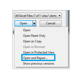 STEP 5 – Click on the Open and Repair option. If this option seems to be impossible to open, do not worry, just check that you have selected the Excel file.
STEP 6 – Click on Repair if you wish to recover most of the workbook data.
Some PC issues are hard to tackle, especially when it comes to corrupted repositories or missing Windows files. If you are having troubles fixing an error, your system may be partially broken.
We recommend installing Restoro, a tool that will scan your machine and identify what the fault is.
Click here to download and start repairing.
Pay attention that you could not have the Repair option. If this is the case, click on Extract Data and pick Convert to Values or Recover Formulas to extract values and formulas from the workbook. In this way, no matter what, you will keep your data.
— RELATED: Excel Online won’t calculate/ open [Best Solutions]
Solution 3 – Recover your data
You may need to recover your data while the corrupted workbook is open. Besides extracting the data, you could go with another procedure in order to recover as much data as you can. Doing that, the corrupted cells will not damage the entire work.
The software should have saved automatically from time to time your work in Excel. Normally, you should have saved as well from time to time your work (Never forget to do so). So, you can take advantage of it, switching back to the last saved version.
STEP 1 – Click on File and Open
STEP 2 – Click two times the workbook you keep open in Excel
STEP 3 – Select Yes to open again the workbook.
The workbook should open without any changes that could have caused the corruption of your cells or of the entire workbook.
Solution 4 – Copy the file in WordPad
If none of the previous solutions worked, there is another option to try to save the data: open the workbook in WordPad. The latter will transform the Excel into text, so no formulas will be recovered.
Nevertheless, WordPad will keep the macros. Wordpad is preferable to Microsoft Word. In fact, if you convert the file in Word, you could find limitation to your data recovering process.
Conclusion
The cell or workbook corruption problem can ruin your day. We hoped this article have solved your problem. Let us know if this was useful by leaving a comment in the space below.
RELATED GUIDES YOU NEED TO CHECK OUT:
- FIX: Compile error in hidden module in Word and Excel
- Microsoft Excel is waiting for another application to complete an OLE action [FIX]
- High CPU usage in Excel? We’ve got the solutions to fix it
![]()
Newsletter
If you are using MS Excel Application of MS Office software and you are facing some issues. Hence, in this blog you will read the solution of Excel Cell Overlapping. You can install MS Excel application of MS Office through www.office.com/setup.

click here to download
Solution To Fix Excel Cell Overlapping:
1. Use Format Cells Option:
First, you
have to select the excel cells in which you want to fix Excel cells overlapping
problem. Then from the context menu, you should select the Format Cells. Now in
the opened dialog box of Format Cells, you should click on the Alignment. After
this, you will view a horizontal option and from its drop-down list you have to
select the Fill option. Here, you should click on the OK button. Now, you will
see the data which is there in the selected cells won’t spill over.
2. Autofit Columns And Rows:
You can do
this by double tap on the rows and column border. After this, you have to place
your mouse pointer on the right border of your column heading till you see a
double-headed arrow. Now, you should double-tap on the border.
You can do
this by using the AutoFit option of columns and rows:
To Autofit The Column Width:
You should
select one or all columns of your worksheet. Then, you have to go to the Home
tab from the Excel ribbon. Here from the cells group, you should click on the
Format option and then select AutoFit Column Width option.
To Autofit The Row Height:
You have to
select the row in which you are facing issue of Excel cells overlapping. Then,
you have to go to the Home tab from the Excel ribbon. Now from the cells group,
you should click on the Format option and then select AutoFit Row Height
option.
3. Manually Resize The Cell:
You should go to the home option and then
select Format. Then from the drop-down
menu of Format option, you have to select the “Column Width”. Now in the
column, the width field will assigns the width size in pixel and then you
should click on OK.
4. Prevent Excel Cells From Spilling
Over With Wrap Text:
To fix this issue, you should turn on the wrap text option. Then, you have to click on the home. Then from the alignment group, you should click on the Wrap text option. This will make your row taller in size to adjust your long comment. Now, you have to click on the Home option and then select Format and after this, choose Row Height. Here in the opened window, you should assign the value 12.75. This will make your cell text in normal height rows. www.office.com/setup
5. Use The Justify Feature:
You should press the Ctrl+1 button from your
keyboard. Now, this will open the dialog box of Format cells on your computer screen.
Then go to the Alignment tab and now from the vertical section, drop-down list
you should click on the Justify option. After this, you should click on the OK button.
This will prevent Excel cells overlapping.
The above method will help you to solve Excel Cell Overlapping issue. If you need any kind of support, then you can contact to the customer care of MS Office through office.com/setup.
check this link: How You Can Disable Touchscreen in Windows?