How to find values in excel - Word и Excel - помощь в работе с программами

Summary

This step-by-step article describes how to find data in a table (or range of cells) by using various built-in functions in Microsoft Excel. You can use different formulas to get the same result.

Create the Sample Worksheet

This article uses a sample worksheet to illustrate Excel built-in functions. Consider the example of referencing a name from column A and returning the age of that person from column C. To create this worksheet, enter the following data into a blank Excel worksheet.

You will type the value that you want to find into cell E2. You can type the formula in any blank cell in the same worksheet.

	A	B	C	D	E
1	Name	Dept	Age		Find Value
2	Henry	501	28		Mary
3	Stan	201	19
4	Mary	101	22
5	Larry	301	29

Term Definitions

This article uses the following terms to describe the Excel built-in functions:

Term	Definition	Example
Table Array	The whole lookup table	A2:C5
Lookup_Value	The value to be found in the first column of Table_Array.	E2
Lookup_Array -or- Lookup_Vector	The range of cells that contains possible lookup values.	A2:A5
Col_Index_Num	The column number in Table_Array the matching value should be returned for.	3 (third column in Table_Array)
Result_Array -or- Result_Vector	A range that contains only one row or column. It must be the same size as Lookup_Array or Lookup_Vector.	C2:C5
Range_Lookup	A logical value (TRUE or FALSE). If TRUE or omitted, an approximate match is returned. If FALSE, it will look for an exact match.	FALSE
Top_cell	This is the reference from which you want to base the offset. Top_Cell must refer to a cell or range of adjacent cells. Otherwise, OFFSET returns the #VALUE! error value.
Offset_Col	This is the number of columns, to the left or right, that you want the upper-left cell of the result to refer to. For example, «5» as the Offset_Col argument specifies that the upper-left cell in the reference is five columns to the right of reference. Offset_Col can be positive (which means to the right of the starting reference) or negative (which means to the left of the starting reference).

Functions

LOOKUP()

The LOOKUP function finds a value in a single row or column and matches it with a value in the same position in a different row or column.

The following is an example of LOOKUP formula syntax:

=LOOKUP(Lookup_Value,Lookup_Vector,Result_Vector)

The following formula finds Mary’s age in the sample worksheet:

=LOOKUP(E2,A2:A5,C2:C5)

The formula uses the value «Mary» in cell E2 and finds «Mary» in the lookup vector (column A). The formula then matches the value in the same row in the result vector (column C). Because «Mary» is in row 4, LOOKUP returns the value from row 4 in column C (22).

NOTE: The LOOKUP function requires that the table be sorted.

For more information about the LOOKUP function, click the following article number to view the article in the Microsoft Knowledge Base:

How to use the LOOKUP function in Excel

VLOOKUP()

The VLOOKUP or Vertical Lookup function is used when data is listed in columns. This function searches for a value in the left-most column and matches it with data in a specified column in the same row. You can use VLOOKUP to find data in a sorted or unsorted table. The following example uses a table with unsorted data.

The following is an example of VLOOKUP formula syntax:

=VLOOKUP(Lookup_Value,Table_Array,Col_Index_Num,Range_Lookup)

The following formula finds Mary’s age in the sample worksheet:

=VLOOKUP(E2,A2:C5,3,FALSE)

The formula uses the value «Mary» in cell E2 and finds «Mary» in the left-most column (column A). The formula then matches the value in the same row in Column_Index. This example uses «3» as the Column_Index (column C). Because «Mary» is in row 4, VLOOKUP returns the value from row 4 in column C (22).

For more information about the VLOOKUP function, click the following article number to view the article in the Microsoft Knowledge Base:

How to Use VLOOKUP or HLOOKUP to find an exact match

INDEX() and MATCH()

You can use the INDEX and MATCH functions together to get the same results as using LOOKUP or VLOOKUP.

The following is an example of the syntax that combines INDEX and MATCH to produce the same results as LOOKUP and VLOOKUP in the previous examples:

=INDEX(Table_Array,MATCH(Lookup_Value,Lookup_Array,0),Col_Index_Num)

The following formula finds Mary’s age in the sample worksheet:

=INDEX(A2:C5,MATCH(E2,A2:A5,0),3)

The formula uses the value «Mary» in cell E2 and finds «Mary» in column A. It then matches the value in the same row in column C. Because «Mary» is in row 4, the formula returns the value from row 4 in column C (22).

NOTE: If none of the cells in Lookup_Array match Lookup_Value («Mary»), this formula will return #N/A.
For more information about the INDEX function, click the following article number to view the article in the Microsoft Knowledge Base:

How to use the INDEX function to find data in a table

OFFSET() and MATCH()

You can use the OFFSET and MATCH functions together to produce the same results as the functions in the previous example.

The following is an example of syntax that combines OFFSET and MATCH to produce the same results as LOOKUP and VLOOKUP:

=OFFSET(top_cell,MATCH(Lookup_Value,Lookup_Array,0),Offset_Col)

This formula finds Mary’s age in the sample worksheet:

=OFFSET(A1,MATCH(E2,A2:A5,0),2)

The formula uses the value «Mary» in cell E2 and finds «Mary» in column A. The formula then matches the value in the same row but two columns to the right (column C). Because «Mary» is in column A, the formula returns the value in row 4 in column C (22).

For more information about the OFFSET function, click the following article number to view the article in the Microsoft Knowledge Base:

How to use the OFFSET function

Need more help?

Want more options?

Explore subscription benefits, browse training courses, learn how to secure your device, and more.

Communities help you ask and answer questions, give feedback, and hear from experts with rich knowledge.

Источник

Transcript

In this lesson, we’ll look at how to find things in Excel.

Let’s take a look.

To find a value in Excel, use the Find and Replace dialog box. You can access this dialog using the keyboard shortcut control-F, or, by using the Find and Select menu at the far right of the Home tab on the ribbon.

Let’s try looking for the name Ann. Nothing happens until we click the Find Next button. Then, each time we click, Excel finds another match.

Note that Excel finds other names that contain Ann as well—Annie, Ann, Danny, and then Hannah. If we continue clicking Find Next, Excel will eventually return to the first match.

By default, Excel searches left to right, first through rows, then columns. You can hold down the shift key when you press «Find Next» to move backwards.

Now let’s review the Find options.

The first option allows you to restrict the search to the current worksheet, or expand it to include the entire workbook. If we select workbook, Excel will now find matches on Sheet 2.

The «search» option determines the order that Excel looks through cells. The default is «By Rows.» If we switch to «By Columns,» Excel will find all matches in one column before moving on to the next column.

There is also an option to search Formulas, Values, and Comments. We’ll look at these in a future lesson.

If we enable «Match case,» Excel treats case as important and only finds values that begin with a capital A.

If we enable «Match entire cell contents,» Excel will only find cells where the value is exactly Ann. This is a good way to find only the name Ann.

With the Find dialog closed, you can still find things with the keyboard shortcut Shift F4. Excel will use the current Find settings and select the next match.

Finally, it’s important to understand that if you have more than one cell selected, Excel will search only in the current selection. For example, if we select just a subset of our table, Excel will only search in that selection.

However, if you switch «Within» to «Workbook,» Excel will drop the current selection and search all cells. At this point, you can switch back to Worksheet to search only the current worksheet.

Источник

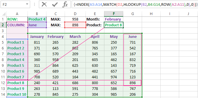
We have the table in which the sales volumes of certain products are recorded in different months. It is necessary to find the data in the table, and the search criteria will be the headings of rows and columns. But the search must be performed separately by the range of the row or column. That is, only one of the criteria will be used. Therefore, you can`t apply the INDEX function here, but you need a special formula.

Finding values in the Excel table

To solve this problem, let us illustrate the example in the schematic table that corresponds to the conditions are described above.

The sheet with the table to search for values vertically and horizontally:

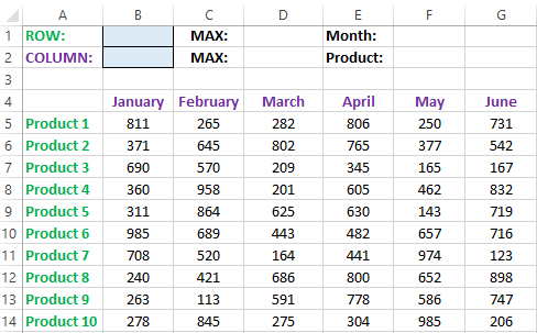
Above this table we can see the row with results. In the cell B1 we introduce the criterion for the search query, that is, the column header or the ROW name. And in the cell D1, to a search formula should return to the result of the calculation of the corresponding value. Then the second formula will work in the cell F1. She will already use the values of the cells B1 and D1 as the criteria for searching of the corresponding month.

Search of the value in the Excel ROW

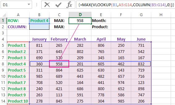
Now we are learning, in what maximum volume and in what month has been the maximum sale of the Product 4.

To search by columns:

In the cell B1 you need to enter the value of the Product 4 — the name of the row, that will act as the criterion.
In the cell D1 you need to enter the following:
To confirm after entering the formula, you need to press the CTRL + SHIFT + Enter hotkey combination, because she must be executed in the array. If everything is done correctly, the curly braces will appear in the formula ROW.

In the cell F1 you need to enter the second:
For confirmation, to press the key combination CTRL + SHIFT + Enter again.

found.

So we have found, in what month and what was the largest sale of the Product 4 for two quarters.

The principle of the formula for finding the value in the Excel ROW:

In the first argument of the VLOOKUP function (Vertical Look Up), indicates to the reference to the cell, where the search criterion is located. In the second argument indicates to the range of the cells for viewing during in the process of searching.

In the third argument of the VLOOKUP function should be indicated the number of the column from which you should to take the value against of the row named the Item 4. But since we do not previously know this number, we use the COLUMN function for creating the array of column numbers for the range B4:G15.

This allows the VLOOKUP function to collect the whole array of values. As a result, all relevant values are stored in memory for each column in the row Product 4 (namely: 360; 958; 201; 605; 462; 832). After that, the MAX function will only take the maximum number from this array and return it as the value for the cell D1, as the result of calculating.

As you can see, the construction of the formula is simple and concise. On its basis, it is possible in a similar way to find other indicators for a certain product. For example, the minimum or an average value of sales volume you need to find using for this purpose MIN or AVERAGE functions. Nothing hinders you from applying this skeleton of the formula to apply with more complex functions for implementation the most comfortable analysis of the sales report.

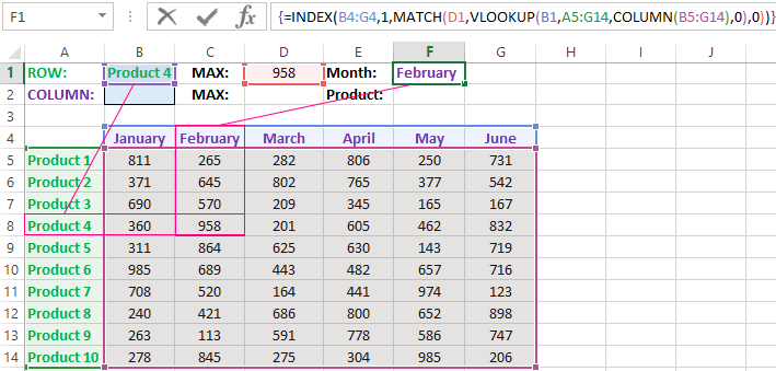
How can I get to the column headings from a single cell value?

For example, how effectively we displayed the month with the maximum sale, using of the second. It’s not difficult to notice that in the second formula we used the skeleton of the first formula without the MAX function. The main structure of the function is: VLOOKUP. We replaced the MAX on the MATCH, which in the first argument uses the value obtained by the previous formula. It acts as the criterion for searching for the month now.

And as a result, the MATCH function returns the column number 2, where the maximum value of the sales volume for the product is located for the product 4. After that, the INDEX function is included in the work. This function returns the value by the number of terms and column from the range specified in its arguments. Because the we have the number of column 2, and the row number in the range where the names of months are stored in any cases will be the value 1. Then we have the INDEX function to get the corresponding value from the range of B4:G4 — February (the second month).

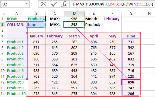
Search the value in the Excel column

The second version of the task will be searching in the table with using the month name as the criterion. In such cases, we have to change the skeleton of our formula: the VLOOKUP function is replaced by the HLOOKUP (Horizontal Look Up) one, and the COLUMN function is replaced by the row one.

This will allow us to know what volume and what of the product the maximum sale was in a certain month.

To find what kind of the product had the maximum sales in a certain month, you should:

In the cell B2 to enter the name of the month June — this value will be used as the search criterion.
In the cell D2, you should to enter the formula:
To confirm after entering the formula you need to press the combination of keys CTRL + SHIFT + Enter, as this formula will be executed in the array. And the curly braces will appear in the function ROW.

In the cell F1, you need to enter the second:
You need to click CTRL + SHIFT + Enter for confirmation again.

Exaple.

The principle of the formula for finding the value in the Excel column

In the first argument of the HLOOKUP function, we indicate to the reference by the cell with the criterion for the search. In the second argument specifies the reference to the table argument being scanned. The third argument is generated by the ROW function, what creates in the array of ROW numbers of 10 elements in memory. So there are 10 rows in the table section.

Further the HLOOKUP function, alternately using to each number of the row, creates the array of corresponding sales values from the table for the certain month (June). Further, the MAX function is left only to select the maximum value from this array.

Then just a little modifying to the first formula by using the INDEX and MATCH functions, we created the second function to display the names of the table rows according to the cell value. The names of the corresponding rows (products) we output in F2.

ATTENTION! When using the formula skeleton for other tasks, you need always to pay attention to the second and the third argument of the search HLOOKUP function. The number of covered rows in the range is specified in the argument, must match with the number of rows in the table. And also the numbering should begin with the second ROW!

Download example search values in the columns and rows

Read also: The searching of the value in a range Excel table in columns and rows

Indeed, the content of the range generally we don’t care — we just need the row counter. That is, you need to change the arguments to: ROW(B2:B11) or ROW(C2:C11) — this does not affect in the quality of the formula. The main thing is that — there are 10 rows in these ranges, as well as in the table. And the numbering starts from the second row!

Источник

The FIND function is a built-in Worksheet Function (WS) in Microsoft Excel, which you can use to locate a sub-string or a specific character’s position within a text string. It is categorized as a TEXT function in Excel.

If the FIND function fails to find the text, it will return a #VALUE error. Note that the Excel FIND function will perform a case-sensitive search.

Excel FIND function is commonly used by financial analysts for locating specific data or text occurrences in a cell.

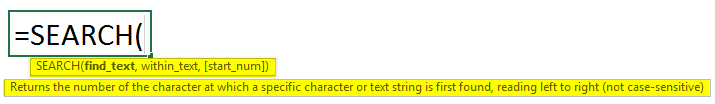
Syntax of Excel FIND function

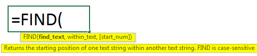
=FIND(find_text, within_text, [start_num])

Arguments:

'find_text' – The text/sub-string you want to locate.
'within_text' – This argument is the string within which you wish to perform the search. You can supply a cell reference or type in the string into the formula.
'start_num' – This is an optional argument wherein you specify the character from which your search must begin. If you omit this argument, the function will assume this parameter as 1, i.e., the search will begin from the 1st character of the 'within_text' string.

Things to Remember

The FIND function in Excel is case-sensitive and does not allow the usage of wildcard characters. For locating case-insensitive matches, take a look at the SEARCH function.
The FIND function will search the 'find_text' argument in 'within_text' and return the first character’s position.
You may search for either a substring or a character with the 'find_text'argument. You may use cell references or text characters for both 'find_text' and 'within_text' The FIND function will return ‘1’ when the 'find_text' argument is an empty string «».
The FIND function returns #VALUE! error when:
- The FIND function cannot locate 'find_text'in 'within_text' or
- The 'start_num' argument is negative, 0, or greater than the length of 'within_text'

Examples of FIND function in Excel

Example 1 – Finding a word’s position in a text string

In this example, when you search for «Dallas» and reference the cell A2, which has the text string «Dallas, USA» the function will return ‘1’. Here, 1 represents the position of the searched word’s starting point.

On account of the FIND function’s case-sensitivity, entering «dallas» as an argument will return #VALUE! error.

Example 2 – Search for a word in a text string

The 'start_num' argument lets you decide the starting position for performing the search in the text string. You will see that in the above example, the FIND function returns ‘1’ when we put 1 as the 'start_num'. Essentially, it searches for the text «Dallas» in «Dallas, USA».

When we change 'start_num' to ‘2’, it returns an error because it then searches for «Dallas» in «allas, USA».

Note that skipping the 'start_num' argument will result in the FIND function assuming ‘1’ as the starting position.

Example 3 – When the searched text occurs multiple times in a text string

Since the FIND function refers to the 'start_num' argument to see if you would like to define a starting position, it returns ‘1’ when you input 'start_num' as 1. This is because it finds «Dallas» at position ‘1’ in «Dallas, Dallas, USA».

When you input 'start_num' as 2, though, you will see that it returns ‘9’. What is happening here is that the FIND function tries to look for the word «Dallas» in «allas, Dallas, USA» since you are asking the function to start searching from the second position. Here, 9 is the starting position of the 2nd «Dallas» in «Dallas, Dallas, USA».

Example 4 – Look for a specific character’s Nth occurrence in a string.

Let’s now assume that you would like to know the position of the second «,» in the list that has the format «City, Country, Continent».

For this, we will need to nest two FIND functions one within another. The second FIND function will go in the first FIND function as a third argument ('start_num'), like so:

=FIND(",",A2,FIND(",",A2)+1)

With the third argument, you are instructing the first FIND function to start searching for «,» exactly after the first occurrence of a «,» in the string.

Pro tip: You can use the CHAR and SUBSTITUTE functions to do this more simply, with the following formula:

=FIND(CHAR(1), SUBSTITUTE(A5,",",CHAR(1),2)

Example 5 – Retrieving the first part of a text string separated by «,» (comma)

Let’s assume you want the list of just the name of cities, without the name of the country, i.e., the characters right before «,»).

To accomplish this, we will use the LEFT function and the FIND function together. The FIND function will give us the position of «,» and the LEFT function will allow us to retrieve the name of the cities.

In our example, the FIND function will return 10 when executed on «Amsterdam, Netherlands». From this, we will subtract 1 since we don’t want to include the «,» in our output.

Next, we embed a FIND function into the LEFT function and use FIND(",", A2,1)-1 as the second argument, like so:

=LEFT(A2,FIND(",",A2,1)-1)

Example 6 – Retrieving the second part of a text string separated by «,» (comma)

Let’s take example 5, and try to retrieve the second part of the string.

To accomplish this, we will use the MID function and the FIND function together. The FIND function will give us the position of «,» and the MID function will allow us to fetch the specific string portion that we need.

In our example, the FIND function will return 10 when executed on «Amsterdam, Netherlands». From this, we will add 1 since we don’t want to include the «,» in our output.

Next, we use a MID function and pass the FIND function to it FIND(",", A2,1)+1 as the second argument, like so:

=MID(A2,FIND(",",A2,1)+1,100)

FIND function vs. SEARCH function in Excel

Both Find and Search functions have a similar syntax and application. However, there are 2 differences between these functions. Let’s dive into what these differences are:

1. Acceptance of wildcard characters

Unlike with the FIND function, you may use wildcard characters in the SEARCH function’s 'find_text' argument.

To match one character – we will use a question mark ‘?’, and to match a series of characters – we will use an asterisk mark ‘*’.

Let’s work this out with an example:

We will use the syntax:

=SEARCH(",*EUROPE",A2)

Notice how the Excel SEARCH function returns the first character’s position if you input both «,» and the «continent name» regardless of how many characters exist between the text string referred to in the 'within_text'argument.

Pro tip: For finding a ‘?’ or ‘*’, just add a tilde (~) in front of the question mark or the asterisk.

2. FIND is case-sensitive, while SEARCH is case-insensitive

As I mentioned previously, case-sensitivity is another differentiating factor between the two functions.

In our example, when using the FIND function to search for ‘A’ it returns the position of the capital A in ‘USA’. However, searching for ‘A’ with the SEARCH function returns the position of the ‘a’ in ‘Dallas’ because it is case-insensitive.

Handling #VALUE! errors in the FIND function

To deal with #VALUE! errors, we can use the IFERROR function.

Let’s revisit our first example where we first encountered a #VALUE! error with FIND function on account of the FIND function’s case-sensitivity.

Here is the syntax we will use to fix this:

=IFERROR(FIND("dallas",A3,1), "Not Found!")

Using this syntax, we will «trap» the error and replace it with a standard string in the second argument of the IFERROR function, which in our case is «Not Found!». So, until the FIND function is able to return a matched string, the function will keep returning «Not Found».

Источник

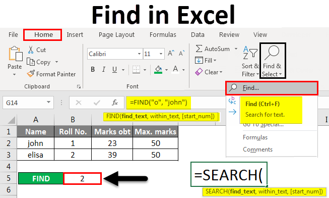
Find in Excel (Table of Contents)

Using Find and Select Feature in Excel
FIND Function in Excel
SEARCH Function in Excel

Introduction to Find in Excel

There are two ways to find it in Excel. First, we can use Find by pressing Ctrl + F shortcut keys. Therein Find and Replace box, search the word or field which we want to find in the Find What section. In another way, we can use the FIND function. For this, select the Find function from the insert function and, as per syntax, select the substring from where we need to find it, and choose the word or letter or number which we want to find in the String position. This will return the position of the chosen string from the selected Substring.

Methods to Find in Excel

Below are the different methods to find in excel.

You can download this Find in Excel Template here – Find in Excel Template

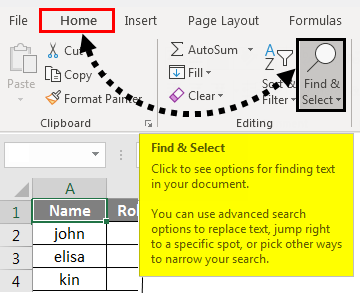
Method #1 – Using Find and Select Feature in Excel

Let’s see How to Find a Number or a Character in Excel using the Find and Select feature in Excel.

Step 1 – Under the Home tab, in the Editing group, click Find & Select.

Step 2 – To find text or numbers, click Find.

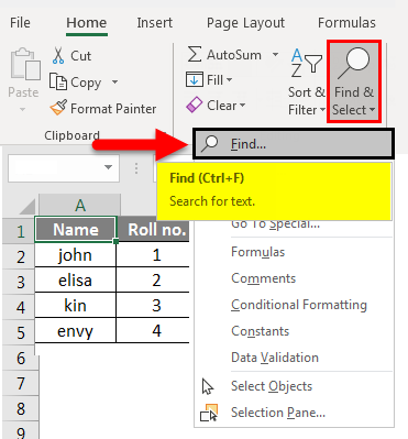
In the Find what box, type the text or character you want to search for, or click the arrow in the Find what box and then click a recent search in the list.

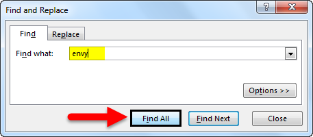
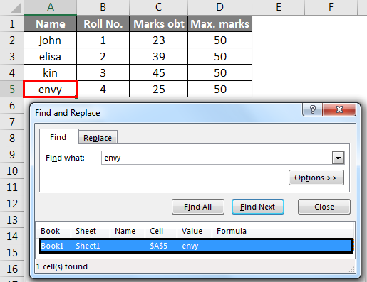
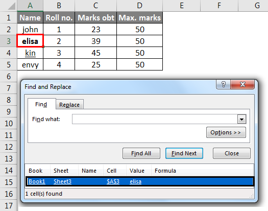
Here, we have a record of marks of four students. Suppose we want to find the text ‘envy’ in this table. For this, we click Find and Select under the Home tab then the Find and Replace dialog box appears. In the Find what box, we enter ‘envy’ then click on Find All. We get the text ‘envy’ is in cell number A5.

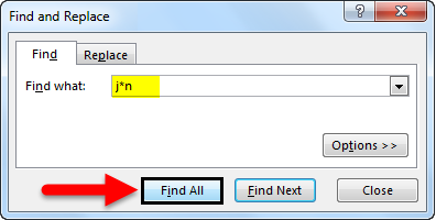
You can use wildcard characters, such as an asterisk (*) or a question mark (?), in your search criteria:

Use the asterisk to find any string of characters.

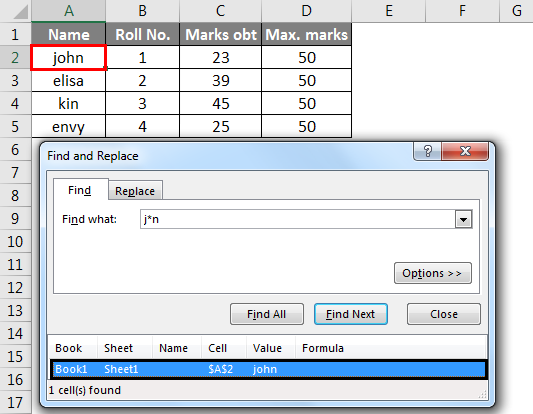
Suppose we want to find text in the table which starts with the letter ‘j’ and ends with the letter ‘n’. In the Find and Replace dialog box, we enter ‘j*n’ in the Find what box, then click on Find All.

We will get the result as text ‘j*n’(john) is in the cell no. ‘A2’ because we have only one text which starts with ‘j’ and ends with ‘n’ with any number of characters between them.

Use the question mark to find any single character.

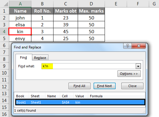
Suppose we want to find text in the table that starts with the letter ‘k’ and ends with the letter ‘n’ with a single character. So, in the Find and Replace dialog box, we enter ‘k?n’ to find what box. Then click on Find All.

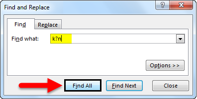
Here, we get the text ‘k?n’(kin) is in cell no. ‘A4’ because we have only one text which starts with ‘k’ and ends with ‘n’ with a single character between them.

Click Options to further define your search if needed.
We can find text or number by changing settings in the Within, Search and Look in the box according to our needs.
To show the working of the above-mentioned options, we took the data as follows.

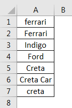
To search case-sensitive data, select the Match case check box. It gives you output in the case you give input in the Find What box. For example, we have a table of some cars’ names. If you type ‘ferrari’ in the Find What box, then it will find only ‘ferrari’, not ‘Ferrari’.

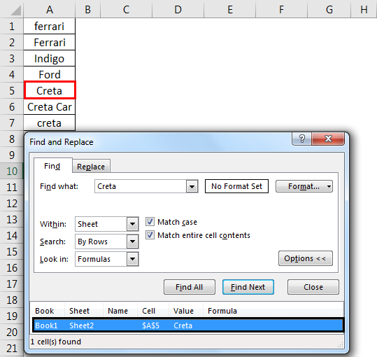
To search for cells that contain just the characters you typed in the Find what box, select the Match entire cell contents checkbox. For example, we have a table of some cars’ names. Type ‘Creta’ in the Find What box.

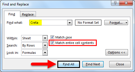
It will then find cells containing exactly ‘Creta’, and cells containing ‘Cretaa’ or ‘Creta car’ will not be found.

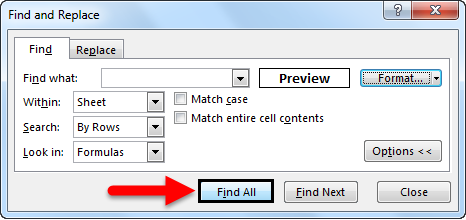
If you want to search for text or numbers with specific formatting, click Format, and then make your selections in the Find Format dialog box according to your need.
Let us click the Font option and select the Bold, and click OK.

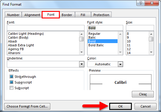
Then, we click on Find All.

We get the value as ‘elisa’, which is in the ‘A3’ cell.

Method #2 – Using FIND Function in Excel

The FIND function in Excel gives the location of a substring within a string.

Syntax For FIND in Excel:

The first two parameters are required, and the last parameter is non-compulsory.

Find_Value: The substring which you want to find.
Within_String: The string in which you want to find the specific substring.
Start_Position: It is a non-compulsory parameter and describes from which position we want to search substring. If you do not describe it, then start the search from the 1^stposition.

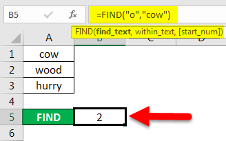
For example =FIND(“o”, “Cow”) gives 2 because “o” is the 2^ndletter in the word “cow“.

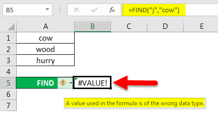
FIND(“j”, “Cow”) gives an error because there is no “j” in “Cow”.

If the Find_Value parameter contains multiple characters, the FIND function gives the location of the first character.

E.g., the formula FIND(“ur”, “hurry”) gives 2 because “u” in the 2^nd letter in the word “hurry”.

If Within_String contains multiple occurrences of Find_Value, the first occurrence is returned. For example, FIND (“o”, “wood”)

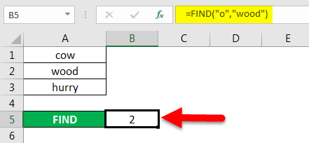
gives 2, which is the location of the first “o” character in the string “wood”.

The Excel FIND function gives the #VALUE! error if:

If Find_Value does not exist in Within_String.
If Start_Position contains multiple characters as compared to Within_String.
If Start_Position either has a zero or negative number.

Method #3 – Using SEARCH Function in Excel

The SEARCH function in Excel is simultaneous to FIND because it also gives the location of a substring in a string.

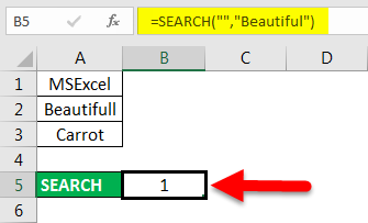
If Find_Value is the blank string “, the Excel FIND formula gives the string’s first character.

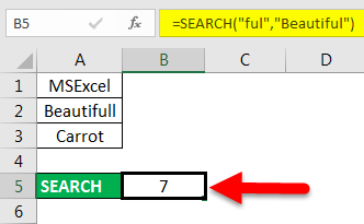
Example =SEARCH (“ful“, “Beautiful) gives 7 because the substring “ful” begins at the 7^th position of the substring “beautiful”.

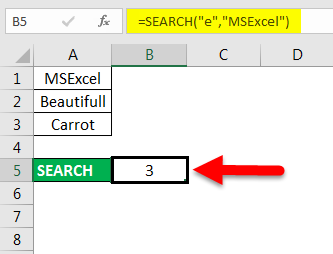
=SEARCH (“e”, “MSExcel”) gives 3 because “e” is the 3rd character in the word “MSExcel” and ignoring the case.

Excel’s SEARCH function gives the #VALUE! error if:

If the value of the Find_Value parameter is not found.
If the Start_Position parameter is superior to the length of Within_String.
If the Start_Position either equal to or less than 0.

Things to Remember About Find in Excel

Asterisk defines a string of characters, and the question mark defines a single character. You can also find asterisks, question marks, and tilde characters (~) in worksheet data by preceding them with a tilde character inside the Find what option.

For example, to find data that contain “*”, you would type ~* as your search criteria.

If you want to find cells that match a specific format, you can delete any criteria in the Find what box and select a specific cell format as an example. Click the arrow next to Format, click Choose Format From Cell, and click the cell with the formatting you want to search for.
MSExcel saves the formatting options you define; you should clear the formatting options from the last search by clicking on an arrow next to Format and then Clear Find Format.
The FIND function is case sensitive and does not allow while using wildcard characters.
The SEARCH function is case-insensitive and allows while using wildcard characters.

Syntax of the FIND Function of Excel

The syntax of the FIND function of Excel is shown in the following image:

The FIND function of Excel accepts the following arguments:

Find_text: This is the character (or substring) whose position is to be searched. It can be supplied as a reference to a cell containing the substring or as a direct substring enclosed within double quotation marks.
Within_text: This is the text string within which the character (or substring) needs to be searched. It can be supplied either directly to the FIND function or as a reference to a cell containing the text string. Enclose the text string within double quotation marks when supplied directly to the function.
Start_num: This is the character from which the search shall begin. It is supplied as a numeric value to the FIND function. For instance, if this argument is 3, the search begins from the third character of the “within_text” argument.

The arguments “find_text” and “within_text” are required, while “start_num” is optional. If the “start_num” argument is omitted, the search begins from the first character of the “within_text” argument.

How to use the FIND Function in Excel?

Let us consider some examples to understand the working of the FIND function in Excel.

You can download this FIND Function Excel Template here – FIND Function Excel Template

Example #1–Find a Single Character Within a Text String

The following image shows a text string and substring in cells A3 and B3 respectively. Within the text string (leopard), we want to find the substring (a) by using the FIND function of Excel. Supply the “find_text” and “within_text” arguments as:

Cell references
Direct strings

Consider the “start_num” argument to be 1 in both cases.

a. The steps to use the FIND function with cell referencesCell reference in excel is referring the other cells to a cell to use its values or properties. For instance, if we have data in cell A2 and want to use that in cell A1, use =A2 in cell A1, and this will copy the A2 value in A1.read more are listed as follows:

Step 1: Supply the cell references of the substring and the text string (in the stated sequence) to the FIND function. So, enter the following formula in cell C3.

“=FIND(B3,A3)”

Notice that the “start_num” argument is omitted since it is 1.

Step 2: Press the “Enter” key. The output appears, as shown in the following image. Hence, the character “a” is the fifth letter of the word “leopard.”

b. The steps to use the FIND function with direct strings are listed as follows:

Step 1: Supply the substring and the text string (in the stated sequence) to the FIND function directly. So, enter the following formula in cell C4.

“=FIND(“a”, “Leopard”)”

Since the “start_num” argument is 1, it has been omitted.

Step 2: Press the “Enter” key. The output in cell C4 is 5. This is shown in the following image. Hence, whether the first two arguments are entered as cell references or direct strings, the output of the FIND function is the same.

Example #2–Count the Number of Times a Single Character Occurs in a Range

The following image shows some random text strings in the range A3:A6. We want to find the number of times the character (or substring) “i” appears in this range. Use the FIND, ISNUMBER, and SUMPRODUCT functions of Excel.

The steps to find the character count by using the stated functions are listed as follows:

Step 1: Enter the following formula in cell B3.

“=SUMPRODUCT(- -(ISNUMBER(FIND(“i”,A3:A6))))”

Step 2: Press the “Enter” key. The output in cell B3 is 3. This is shown in the following image. Hence, the character “i” appears thrice in the range A3:A6.

Explanation: In the formula entered in step 1, the FIND function is processed first as it is the innermost function. Next, the ISNUMBERISNUMBER function in excel is an information function that checks if the referred cell value is numeric or non-numeric.read more and SUMPRODUCTThe SUMPRODUCT excel function multiplies the numbers of two or more arrays and sums up the resulting products.read more functions are processed. The entire formula works as follows:

The FIND function looks for the character “i” in each cell of range A3:A6. This character is found in cells A3, A4, and A6. It is not found in cell A5. If the character “i” is found in a cell, the FIND function returns its position. However, if this character is not found in a cell, the FIND function returns the “#VALUE!” error. So, the FIND function returns an array of four values {3;5;#VALUE!;5 }.
The array returned by the FIND function becomes an argument of the ISNUMBER function. If the output of the FIND function is numeric, the ISNUMBER returns “true.” However, if the output of the FIND function is an error, the ISNUMBER function returns “false.” So, the ISNUMBER returns an array of Boolean values {TRUE;TRUE;FALSE;TRUE}.
The unary operator or the double negative symbol (- -) converts every “true” and “false” output of the ISNUMBER function into 1 and 0 respectively. So, the unary operator returns a vertical array of four numbers {1;1;0;1}.
The array ({1;1;0;1}) returned by the unary operator becomes an argument of the SUMPRODUCT function. Since it is a single array of numbers, the SUMPRODUCT sums it. So, the sum returned by the SUMPRODUCT function is 3.

Hence, the final output of the given formula (entered in step 1) is 3.

Notice that three cells of the range A3:A6 contained a single instance of the character “i.” However, had there been multiple occurrences of this character in cells A3, A4 or A6, the FIND function would have returned its first instance. Therefore, the final output would still have been 3.

Note 1: The ISNUMBER function checks whether a value (or a cell containing a value) is numeric or not. The SUMPRODUCT function multiplies the numbers of two or more arrays and sums up the resulting products. In case of a single array, the SUMPRODUCT function adds the numbers and returns their sum.

For the syntax of the ISNUMBER and SUMPRODUCT functions, click the hyperlinks given in the preceding explanation.

Note 2: Rather than the FIND function, one could have used the COUNTIFThe COUNTIF function in Excel counts the number of cells within a range based on pre-defined criteria. It is used to count cells that include dates, numbers, or text. For example, COUNTIF(A1:A10,”Trump”) will count the number of cells within the range A1:A10 that contain the text “Trump”
read more function. The formula for counting the character “i” in the range A3:A6 would be =COUNTIF(A3:A6,“*i*”). This formula would also have returned the output 3.

Like the FIND function, the COUNTIF would also have returned 3 in case of multiple occurrences of character “i” in cells A3, A4 or A6. However, the COUNTIF is not case-sensitive, unlike the FIND function.

Example #3–Count the Text Strings Ending With Certain Characters

The following image shows a list of names in column A. We want to find the number of names ending with “ansh” or “anka” in the range A3:A10. Use the FIND, ISNUMBER, and SUMPRODUCT functions of Excel.

The steps to count specific names by using the stated functions are listed as follows:

Step 1: Enter the following formula in cell B3.

“=SUMPRODUCT(- -((ISNUMBER(FIND(“ansh”,A3:A10))+ISNUMBER(FIND(“anka”,A3:A10)))>0))

Step 2: Press the “Enter” key. The output in cell B3 is 4. This is shown in the following image.

Hence, a total of 4 names end with “ansh” or “anka.” Two names end with the former substring (Priyansh and Divyansh) and two names end with the latter substring (Priyanka and Divyanka).

Explanation: The formula entered in step 1 is explained as follows:

The FIND function processes each name of the range A3:A10. If “ansh” or “anka” are present in a cell, the FIND function returns the position of the first letter of these substrings. However, if these substrings are not present in a cell, the FIND function returns the “#VALUE!” error. So, the FIND function returns two arrays {#VALUE!;#VALUE!;5;5;#VALUE!;#VALUE!;#VALUE!; #VALUE!} and {5;5;#VALUE!;#VALUE!;#VALUE!;#VALUE!;#VALUE!;#VALUE!}.
The ISNUMBER processes the outputs returned by the FIND function. If the output of the FIND function is numeric, the ISNUMBER returns “true,” otherwise returns “false.” So, the ISNUMBER function returns two arrays {FALSE;FALSE;TRUE;TRUE;FALSE;FALSE;FALSE;FALSE} and {TRUE;TRUE;FALSE;FALSE;FALSE;FALSE;FALSE;FALSE}.
The two arrays returned by the ISNUMBER function are added due to the “plus” operator placed between them. The array returned after addition and the application of the “greater than zero” expression is {TRUE;TRUE;TRUE;TRUE;FALSE;FALSE;FALSE;FALSE}.
The unary operator (- -) converts each “true” and “false” output of the preceding array to 1 and 0 respectively. So, the unary operator returns the final array of 8 values {1;1;1;1;0;0;0;0}.
The SUMPRODUCT function sums the single array returned by the unary operator. Hence, this function returns the output 4.

Note 1: The “greater than zero” expression checks whether each output of the two arrays (returned by the ISNUMBER function) is greater than zero or not. This expression is useful in case one requires logical values (true and false) as the output.

This expression returns “true” if either of the two outputs (of the two arrays returned by the ISNUMBER function) is a number. It returns “false” if both outputs are errors.

Note 2: For knowing more about the ISNUMBER and SUMPRODUCT functions, refer to the hyperlinks (within the explanation) or “note 1” of the preceding example (example #2).

The following image shows some incomplete statements containing a hash symbol (#) in column C. From each statement, we want to extract this symbol, the word following it, and the trailing space in a separate column. Use the MID and FIND functions of Excel.

The steps to extract the given substrings using the stated functions are listed as follows:

Step 1: Enter the following formula in cell D3.

“=MID(C3,FIND(“#”,C3),FIND(” “,(MID(C3,FIND(“#”,C3),LEN(C3)))))”

Step 2: Press the “Enter” key. The output in cell D3 is “#Wedding .” It includes a space at the end. The output is shown in the following image.

Step 3: Drag the formula of cell D3 till cell D5 by using the fill handle. The output of the range D3 to D5 is shown in the following image.

Hence, the hash symbol, the following word, and the trailing space have been extracted from each statement of column C.

Explanation: In the given formula (entered in step 1), each function on the right is processed, followed by the subsequent function on the left. The LEN functionThe Len function returns the length of a given string. It calculates the number of characters in a given string as input. It is a text function in Excel as well as an inbuilt function that can be accessed by typing =LEN( and entering a string as input.read more, being the innermost (or rightmost), is processed first. The entire formula works as follows:

The LEN function counts the total number of characters in cell C3. So, the formula “=LEN(C3)” returns 27. This count includes 23 letters, 3 spaces, and 1 hash symbol.
Next, the FIND function searches the position of the hash symbol in cell C3. So, the formula “=FIND(“#”,C3)” returns 10. This implies that the hash symbol is at the tenth position of the statement given in cell C3.
The outputs of the FIND and LEN functions become the arguments of the MID functionThe mid function in Excel is a text function that finds strings and returns them from any mid-part of the spreadsheet. read more. So, the MID function processes the formula “=MID(C3,10,27)” and returns “#Wedding in Jaipur.”
The output of the MID function becomes the argument of the FIND function. The FIND function searches for a space character in the string “#Wedding in Jaipur.” So, the formula “=FIND(“ ”,“#Wedding in Jaipur”) returns 9. This implies that the first instance of the space character is at the ninth position of the given text string (#Wedding in Jaipur).
The formula “=FIND(“#”,C3)” again returns 10.
The outputs of the two FIND functions (in the preceding two pointers) become the arguments of the MID function. The formula “=MID(C3,10,9)” returns the string beginning from the tenth character and consisting of nine characters in total. So, this formula returns “#Wedding ” including a single space at the end of the word.

Likewise, the outputs in cells D4 and D5 have been returned by Excel.

Note 1: The LEN function counts all the characters in a cell. This includes letters, numbers, spaces, and special characters. The MID function helps extract a certain number of characters from the middle of the string. The position to begin extraction from can be specified to the MID function.

For the syntax of the LEN and MID functions, click the hyperlinks given in the preceding explanation.

Note 2: In the formula “=MID(C3,10,27),” the “start_num” argument is 10 and the “num_chars” argument is 27. If the sum of these two arguments exceeds the total length of the string, the MID function returns the characters beginning from the “start_num” till the end of the entire string.

Therefore, since 37 (“start_num” is 10 and “num_chars” is 27) exceeds 27 (length of the entire string), the MID function returns the character beginning from the tenth place (#) till the end of the string (Jaipur). So, the MID function returns “#Wedding in Jaipur.”

Relevance and Uses of the FIND Function of Excel

The FIND function of Excel is helpful in the following situations:

It helps extract the relevant characters, thereby removing the unwanted substrings of a text string.
It helps extract the words preceding or succeeding a specific character.
It assists in searching the n^th occurrence of a character.
It can be combined with other functions of Excel to find the number of times a character appears in a range.

The important points related to the FIND function of Excel are listed as follows:

The FIND function looks for the first occurrence of the “find_text” in the “within_text” argument.
The “find_text” and “within_text” arguments can be supplied as cell references or direct text strings. To supply these arguments as direct text strings, they must be enclosed within double quotation marks.
If the “find_text” argument contains more than one character, the FIND function returns the position of the first character in the “within_text” argument.
If the “find_text” argument is an empty string (“”), the FIND function returns 1.
The FIND function is case-sensitive and does not support the usage of wildcard characters.
The FIND function returns the “#VALUE!” error in the following cases:
- The “find_text” is not found in the “within_text” argument
- The “start_num” argument is zero or negative
- The “start_num” argument contains more characters than the “within_text” argument

Frequently Asked Questions

1. Define the FIND function of Excel.

The FIND function of Excel returns the position of a character within a text string. The first instance of such character is returned. In case multiple characters are searched within a text string, the position of the first searched character is returned.

The FIND function of Excel returns a numeric value. The function can be told the position from where the search should begin.

Note: For the syntax of the FIND function of Excel, refer to the heading “syntax of the FIND function of Excel” of this article.

2. Is the FIND function of Excel case-sensitive? Explain with the help of an example.

Yes, the FIND function of Excel is case-sensitive. This implies that this function treats the lowercase and uppercase letters differently.

For example, the formula =FIND(“m”,“smile”) looks for the lowercase “m” in the text string “smile.” It returns 2, signifying that “m” is the second letter of the given text string.

However, the formula =FIND(“M”,“smile”) looks for the uppercase “M” in the text string “smile.” It returns the “#VALUE!” error since “M” could not be found in the given text string. Had the text string been supplied as “SMILE,” the FIND function would have again returned 2.

Note: For a case-insensitive function, use the SEARCH in place of the FIND function of Excel.

3. How can the FIND function be used with the LEFT function of Excel?

The LEFT function helps extract the specified number of characters from the leftmost side of a text string. The FIND and LEFT functions can be used together to extract a substring from the left side of a cell. The formula for the same is stated as follows:

“=LEFT(textstring,FIND(character,textstring)-1)”

The “textstring” is the cell reference containing the entire text string. The substring preceding the “character” is extracted. The “-1” ensures that the “character” is not included in the output.

Therefore, if the substring “rose” needs to be extracted from cell A1 containing “rose flower,” the formula used is “=LEFT(A1,FIND(” “,A1)-1).” The “-1” of the formula helps exclude the trailing space of the substring extracted. Had the strings “rose” and “flower” been separated by a hyphen, we would have used the hyphen (“-”) as the “character.”

Note: The given formula should be entered in Excel without the beginning and ending double quotation marks.

FIND Function in Excel Video

Find and Highlight Something

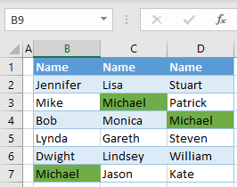
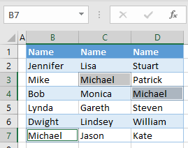
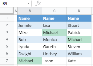
In Excel, you can find all cells containing a specific value and highlight them with the same background color. Say you have the data set pictured below.

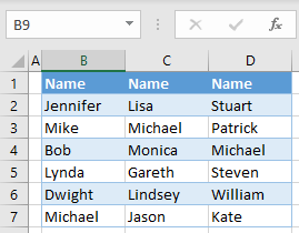
To find all cells containing Michael and apply a green fill, follow these steps.

In the Ribbon, go to Home > Find & Select > Find.

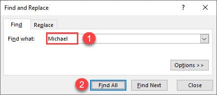
In the Find and Replace window, enter the text you want to find (Michael) and click Find All.

The bottom part of the window, shows all cells where the searched value appears.
Select one line in the found cells and press CTRL + A on the keyboard to select all cells.
Then click Close.

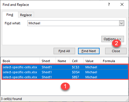
Now that all cells containing Michael are selected (B7, C3, and D4).

To highlight them, in the Ribbon, go to Home > Fill Color > Green Color.

Finally, all cells that contain the text Michael are highlighted in green.

Note: You can also use VBA code to find and highlight cells with a specific value.

Find and Highlight Something in Google Sheets

To find a certain value and highlight in Google Sheets, use conditional formatting.

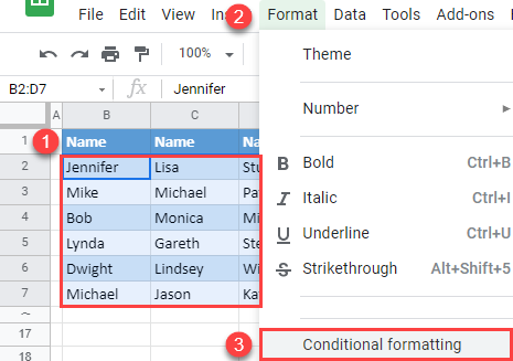
Select the data range where you want to search for a value (B2:D7), and in the Menu, go to Format > Conditional formatting.

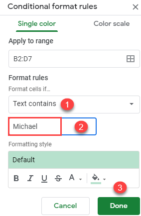
On the right side of the window, select Text contains for Format rules, enter the text to find (e.g., Michael), and click Done.
Leave the default fill color (green). If necessary, you can change it later using the Fill color icon.

Finally, all cells containing Michael have a green background.

Источник

In this article, we will learn How to Find and Replace Multiple Values in Excel.

Scenario:

We know how to find and replace a single item in the sheet at one time. We just press CTRL+H to open the find and replace dialog and use it to replace a single value. But what if we have multiple items to replace with one or multiple items? How do we replace multiple items in Excel? In this article we will learn exactly that. Hold tight.

Generic Formula in Excel

So we remember the SUBSTITUTE function. We used this function to replace a given text in a string with another text. We will use multiple SUBSTITUTE functions to find multiple values and replace multiple values. The SUBSTITUTE will need help from the INDEX function also. So with that said, let’s see the generic formula.

Generic Formula to Find Multiple Items and Replace With One Value

=SUBSTITUTE(SUBSTITUTE(original_text,INDEX(find_list,1),»replacer_text»),
INDEX(find_list,2),»replacer_text»)

Generic Formula to Find Multiple Items and Replace With Multiple Values

=SUBSTITUTE(SUBSTITUTE(original_text,INDEX(find_list,1),INDEX(Replacer_list,1)),
INDEX(E3:E7,2),INDEX(Replacer_list,2))

Here

Original_text: This is the reference of the string in which you want to find and replace multiple items.

Find_list: It is a range that contains the list of items to be found. It can be a named range or absolute reference.

Replacer_list (for multiple replace): It is a range that contains the list of items to be replaced with found items. It can be a named range or absolute reference.

1,2… : These are the index of values to find in the find_list and replacer_list.

Replacer_text (for single replacement): When you want to replace multiple items with one single item, in that case you can have a hardcoded text or single cell reference.

The first generic formula is for finding multiple items and replacing it one text at once. The second generic formula is for finding multiple items and replacing them with multiple items at once.

Example :

All of these might be confusing to understand. Let’s understand how to use the function using an example. Here we can see in the above image, we have an original data that has some random punctuations between numbers. We have the list of these punctuations in range E3:E7 and have named this range as Find.

We need to find each character in the Find list and replace it with a comma (,).

Since we have to find five characters we will need five nested SUBSTITUTE functions. So write the below formula in B3 and drag down.

=SUBSTITUTE(SUBSTITUTE(SUBSTITUTE(SUBSTITUTE(SUBSTITUTE(B3,INDEX(find,1),»,»),
INDEX(find,2),»,»),INDEX(find,3),»,»),INDEX(find,4),»,»),INDEX(find,5),»,»)

Here Find =$E$3:$E$7

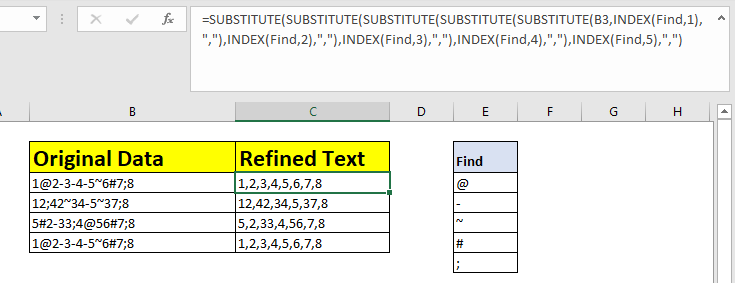
You can see that the data is cleaned. We successfully found multiple items of the list and replaced them with a comma. And we have cleaned data with each number separated with a comma.

How does it work?

Well, the formula may look complex but the technique is quite simple. First we replace one text with another and get the replaced string. Now we take this replaced text string as the original string and do the next replacement using another SUBSTITUTE function.

If we talk in the terms of the above example, this is how it is solved.

=SUBSTITUTE(SUBSTITUTE(SUBSTITUTE(SUBSTITUTE(SUBSTITUTE(B3,»@»,»,»),INDEX(find,2),»,»),
INDEX(find,3),»,»),INDEX(find,4),»,»),INDEX(find,5),»,»)

=SUBSTITUTE(SUBSTITUTE(SUBSTITUTE(SUBSTITUTE(«1,2-3-4-5~6#7;8″,»-«,»,»),INDEX(Find,3),»,»),INDEX(Find,4),»,»),INDEX(Find,5),»,»)

=SUBSTITUTE(SUBSTITUTE(SUBSTITUTE(«1,2,3,4,5~6#7;8″,»~»,»,»),INDEX(Find,4),»,»),
INDEX(Find,5),»,»)

=SUBSTITUTE(SUBSTITUTE(«1,2,3,4,5,6#7;8″,»#»,»,»),INDEX(Find,5),»,»)

=SUBSTITUTE(«1,2,3,4,5,6,7;8″,»;»,»,»)

=»1,2,3,4,5,6,7,8″

Here the INDEX function plays a big role. The INDEX function takes the Find list and in the first iteration (INDEX(find,1)) returns the first value that needs to be found. In the next iteration, it returns the next text that needs to be replaced using INDEX(find,2). And so on. So basically, the INDEX function is used as a feeder to SUBSTITUTE function here that provides values which need to be found and replaced.

Example 2: Find Multiple Items and Replace with Multiple Values

In the above example we had multiple values to find and replace with one value. In this example, we have multiple values to find and replace them with multiple values.

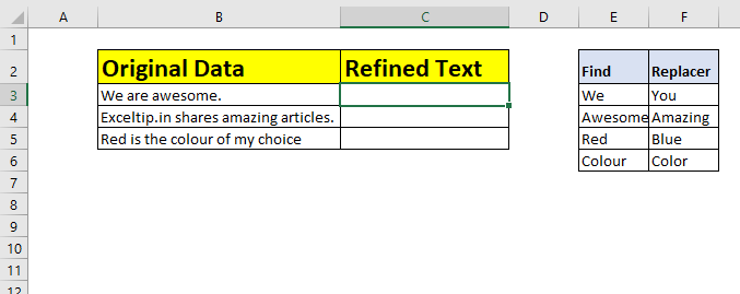
In this example we have a list of items to search and a list of items to replace those items with. How would you do this? You guessed it right. As we used INDEX function to feed the SUBSTITUTE function with find value, we will use INDEX function to feed replacement value too (instead of hardcoded value).

So using the second generic formula we write the below formula in the cell C3 and drag it down.

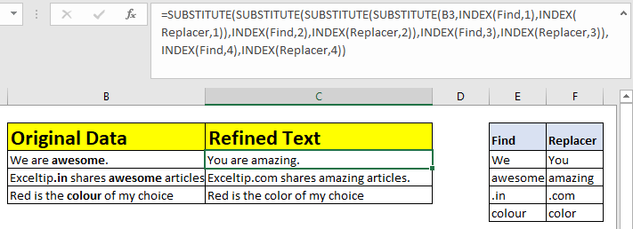
So, how does this work?

It works the same as the first formula. Since we needed to find and replace four values, we have four SUBSTITUTE functions. To find values, we have the same INDEX function. The new thing is another INDEX function, that we use to fetch replacing text.

Let’s see how the formula in cell C4 is solved.

=SUBSTITUTE(SUBSTITUTE(SUBSTITUTE(SUBSTITUTE(B4,»We»,»You»),INDEX(find,2),
INDEX(replacer,2)),INDEX(find,3),INDEX(replacer,3)),INDEX(find,4),INDEX(replacer,4))

=SUBSTITUTE(SUBSTITUTE(SUBSTITUTE(«Exceltip.in shares awesome
articles.»,»awesome»,»amazing»),INDEX(find,3),INDEX(replacer,3)),INDEX(find,4),(replacer,4))

=SUBSTITUTE(SUBSTITUTE(«Exceltip.in shares amazing articles.»,».in»,».com»),
INDEX(find,4),INDEX(replacer,4))

=SUBSTITUTE(«Exceltip.com shares amazing articles.»,»colour», «color»)

=Exceltip.com shares amazing articles.

Here you can see how step by step each substitution is done. The first INDEX pair provides the first find and replacing pair (We and You) and this happens till the last substitution function.

In previous examples, we used the INDEX function only for finding multiple text but in this example we used the INDEX function to fetch replacing text.

The SUBSTITUTE function is case sensitive. If you want a case insensitive formula that finds and replaces multiple values, wrap the original text in LOWER or UPPER function and wrap the old text into the same function.

Formula for finding and replacing multiple items with case insensitive.

=SUBSTITUTE(SUBSTITUTE(UPPER(B3),UPPER(INDEX(find,1)),»,»),UPPER(INDEX(find,2)),»,»))

Here are all the observational notes using the formula in Excel
Notes :

The find and replace text should be sorted in a table. As we use indexes to find and replace, make sure that ‘find’ text has the same index as ‘replace’ text. It is better to have both lists side by side as we have in the second example.
The generic formula has two SUBSTITUTE functions. You will need as many substitute functions as many you have replacements to do.
wildcards help with extracting value from the substrings.
The COUNTIF function supports logical operators like <, >, <>, = but these are used using double quote sign ( « ) with arguments. But if you are using cell reference for the criteria quotes can be ignored.
Criteria argument should use quote sign («) for texts ( like «Gillen» ) or numbers ( like «>50» ).
The formula can be used for both texts and numbers.

Hope this article about How to Find and Replace Multiple Values in Excel is explanatory. Find more articles on calculating values and related Excel formulas here. If you liked our blogs, share it with your friends on Facebook. And also you can follow us on Twitter and Facebook. We would love to hear from you, do let us know how we can improve, complement or innovate our work and make it better for you. Write to us at info@exceltip.com.

Related Articles :

Excel REPLACE vs SUBSTITUTE function: The REPLACE and SUBSTITUTE functions are the most misunderstood functions. To find and replace a given text we use the SUBSTITUTE function. Where REPLACE is used to replace a number of characters in string…

Replace text from end of a string starting from variable position: To replace text from the end of the string, we use the REPLACE function. The REPLACE function use the position of text in the string to replace.

How to Check if a string contains one of many texts in Excel: To check if a string contains any of multiple texts, we use this formula. We use the SUM function to sum up all the matches and then perform a logic to check if the string contains any of the multiple strings.

Count Cells that contain specific text: A simple COUNTIF function will do the magic. To count the number of multiple cells that contain a given string we use the wildcard operator with the COUNTIF function.

Popular Articles :

50 Excel Shortcuts to Increase Your Productivity : Get faster at your tasks in Excel. These shortcuts will help you increase your work efficiency in Excel.

How to use the VLOOKUP Function in Excel : This is one of the most used and popular functions of excel that is used to lookup value from different ranges and sheets.

How to use the IF Function in Excel : The IF statement in Excel checks the condition and returns a specific value if the condition is TRUE or returns another specific value if FALSE.

How to use the SUMIF Function in Excel : This is another dashboard essential function. This helps you sum up values on specific conditions.

How to use the COUNTIF Function in Excel : Count values with conditions using this amazing function. You don’t need to filter your data to count specific values. Countif function is essential to prepare your dashboard.

Источник

You can search in Excel to quickly find terms or numbers in your spreadsheet.
It’s easy to search in Excel by typing into the Search Sheet bar at the top of the screen, or by using a keyboard shortcut.
You can also search for terms or numbers and easily replace them with another value by using Find and Replace.
Visit Business Insider’s homepage for more stories.

Excel spreadsheets are a daunting affair for many.

And indeed, when you are confronting dozens of rows and columns comprising hundreds if not thousands of cells filled with all sorts of data, it’s only logical to be a bit unnerved. How are you going to find that one term or figure among all that clutter?

If you know what you’re searching for, using Excel’s search tools makes finding any term or number tucked into any cell quick and easy.

Here’s how to search an Excel spreadsheet.

Check out the products mentioned in this article:

Microsoft Office (From $139.99 at Best Buy)

MacBook Pro (From $1,299.99 at Best Buy)

Lenovo IdeaPad 130 (From $299.99 at Best Buy)

How to search in Excel using the Search Sheet bar

1. Simply click into the task bar with the faint words «Search Sheet» at the top right corner of the spreadsheet and enter the words or numbers you wish to find.

search1

Click into the search box.

Steven John/Business Insider

2. Hit «Enter» on a PC (or «Return» if you’re using a Mac) to find the first instance, and then use the arrows beside the search term to hop to the next or previous instance.

3. You can also quickly access this search bar by using a «command + F» keyboard shortcut on a Mac, and a «Control + F» shortcut on a PC.

search2

If you can’t find the terms or numbers you’re looking for, be sure to double check the way you typed them into the search bar; Excel won’t look for similar terms, so a mistype ruins the effort.

Steven John/Business Insider

How to use the Replace option to swap in new terms

If you have to replace multiple instances of a term or figure in your Excel sheet, then click on the magnifying glass icon at the top right corner of the screen and click «Replace…»

search3

Select Replace under the magnifying glass.

Steven John/Business Insider

In the pop-up box, enter the term you want to replace into the bar marked «Find what» and the new term (or number) into the «Replace with» bar and then select «Replace All» for a total swap out, or use «Find Next» to go on a case-by-case basis.

search4

You can replace all such terms or toggle through them in the spreadsheet.

Steven John/Business Insider

Related coverage from How To Do Everything: Tech:

How to merge and unmerge cells in Microsoft Excel in 4 ways, to clean up your data and formatting
How to lock cells in Microsoft Excel, so people you send spreadsheets to can’t change certain cells or data
How to alphabetize data in an Excel spreadsheet by column or row, and by using shortcuts
How to freeze a row in Excel so it remains visible when you scroll, to better compare data on different parts of a spreadsheet

Steven John

Freelance Writer

Steven John is a freelance writer living near New York City by way of 12 years in Los Angeles, four in Boston, and the first 18 near DC. When not writing or spending time with his wife and kids, he can occasionally be found climbing mountains. His writing is spread across the web, and his books can be found at www.stevenjohnbooks.com.

Summary

Create the Sample Worksheet

Term Definitions

Functions

LOOKUP()

VLOOKUP()

INDEX() and MATCH()

OFFSET() and MATCH()

Need more help?

Want more options?

Transcript

Finding values in the Excel table

Search of the value in the Excel ROW

The principle of the formula for finding the value in the Excel ROW:

How can I get to the column headings from a single cell value?

Search the value in the Excel column

The principle of the formula for finding the value in the Excel column

Syntax of Excel FIND function

Things to Remember

Examples of FIND function in Excel

FIND function vs. SEARCH function in Excel

1. Acceptance of wildcard characters

2. FIND is case-sensitive, while SEARCH is case-insensitive

Handling #VALUE! errors in the FIND function

Introduction to Find in Excel

Methods to Find in Excel

Method #1 – Using Find and Select Feature in Excel

Method #2 – Using FIND Function in Excel

Method #3 – Using SEARCH Function in Excel

Things to Remember About Find in Excel

Recommended Articles

Table of contents

Syntax of the FIND Function of Excel

How to use the FIND Function in Excel?

Example #1–Find a Single Character Within a Text String

Example #2–Count the Number of Times a Single Character Occurs in a Range

Example #3–Count the Text Strings Ending With Certain Characters

Relevance and Uses of the FIND Function of Excel

Frequently Asked Questions

FIND Function in Excel Video

Recommended Articles

Find and Highlight Something

Find and Highlight Something in Google Sheets

Example 2: Find Multiple Items and Replace with Multiple Values

Check out the products mentioned in this article:

Microsoft Office (From $139.99 at Best Buy)

MacBook Pro (From $1,299.99 at Best Buy)

Lenovo IdeaPad 130 (From $299.99 at Best Buy)

How to search in Excel using the Search Sheet bar

How to use the Replace option to swap in new terms

Related coverage from How To Do Everything: Tech:

How to merge and unmerge cells in Microsoft Excel in 4 ways, to clean up your data and formatting

How to lock cells in Microsoft Excel, so people you send spreadsheets to can’t change certain cells or data

How to alphabetize data in an Excel spreadsheet by column or row, and by using shortcuts

How to freeze a row in Excel so it remains visible when you scroll, to better compare data on different parts of a spreadsheet