
There are many functions in order to find the average in Excel (although it does not matter what kind of value it is: numerical, textual, percentage or other). And each of them has its own peculiarities and advantages. After all, certain conditions can be put in this task.
For example, the average in Excel is counting using statistical functions. You can also manually enter your own formula. Consider the various options.
How to find the arithmetic mean?
It is necessary to add all the numbers in the set and divide the sum by the number in order to find the arithmetic mean. For example, the student’s marks in computer science: 3, 4, 3, 5, 5. The average rating is 4 for a quarter. We found the arithmetic mean using the formula: =(3 + 4 + 3 + 5 + 5) / 5.
How can you quickly do this with Excel functions? Take for example a number of random numbers in a row:

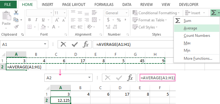
- We put the cursor in cell A2 (under a set of numbers). In the menu – «HOME»-«Editing»-«AutoSum»-«Average» button. A formula appears after clicking in the active cell. Select the range: A1: H1 and press ENTER.
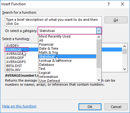
- The second method is based on the same principle of finding the arithmetic mean. But we will call the function AVERAGE differently. Using the function wizard (use fx button or key combination SHIFT + F3).
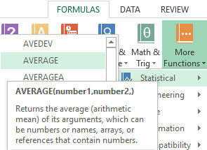
- The third way to call the AVERAGE function from the panel: «FORMULAS»-«More Function»-«Statistical»-«AVERAGE».
Or you can make cell to be active and just manually enter the formula: =AVERAGE(A1:A8).
Now let’s see what the AVERAGE function be able to:
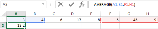
Let us find the arithmetic mean of the first two and three last numbers. Formula: =AVERAGE(A1:B1,F1:H1).
Average value by condition
A numerical criterion or a textual criterion can be the condition for finding the arithmetic mean. We will use the function: = AVERAGEIF().
Find the arithmetic mean for numbers that are greater or equal to 10.
Function:
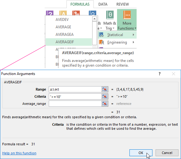
The result of using the function «AVERAGEIF» by the condition «>=10» is next:
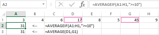
The third argument «Averaging Range» is omitted. Firstly, it is not necessary. Secondly, the range analyzed by the program contains ONLY numeric values. In the cells specified in the first argument, the search will be performed according to the condition specified in the second argument.
Attention! You can specify the search criteria in the cell. And in the formula make a reference to it.
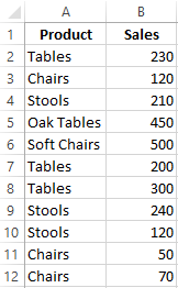
Let’s find the average value of numbers by the text criterion. For example, the average sales of goods «Tables».
The function will look like this:
Range is a column with the names of goods. Search criteria is a link to a cell with the word «Tables» (you can insert the word «Tables» instead of the A7 link). The averaging range is the cells from which data will be taken to calculate the arithmetic mean.
We get the following value as a result of calculating using the function:
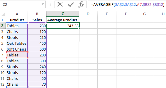
Attention! It is mandatory to point the averaging range for the text criterion (condition).
How to calculate the weighted average price in Excel?
How to calculate the average percentage in Excel? For this purpose, the SUMPRODUCTS and SUM functions are suitable. Table for an example:
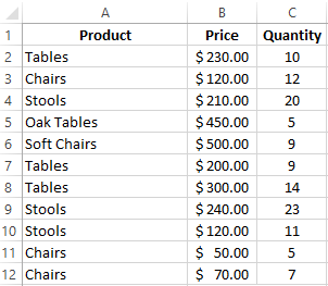
How did we know the weighted average price?
Formula:
Using the formula =SUMPRODUCT() we learn the total revenue after the realization of the entire quantity of goods. And the =SUM() function sums the goods quantity. We found a weighted average price having divided the total revenue from the sale of goods by the total number of units of the goods. This indicator takes into account the «weight» of each price and its share in the total mass of values.
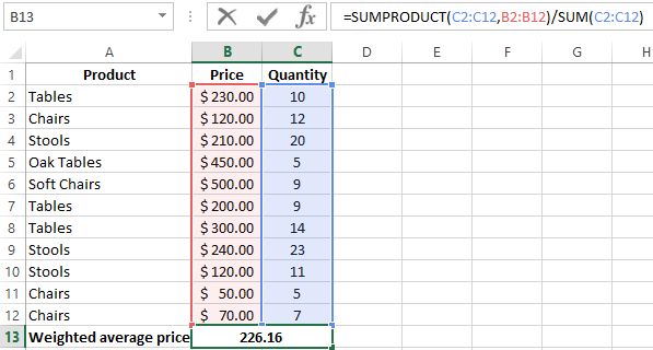
The standard deviation: the formula in Excel
There is a standard deviation in the entire population and in the sampling. In the first case, this is the square root of the general variance. In the second, this is a square root of the sampling variance.
A dispersion formula is compiled to calculate this statistical indicator. The square root is extracted from it. But in Excel, there is a ready-made function for finding the root-mean-square deviation.
The root-mean-square deviation is related to the scope of the initial data. This is not enough for a figurative representation of the variation of the analyzed range. The coefficient of variation is calculated to obtain the relative level of the data variability.
standard deviation / arithmetic mean
The formula in Excel is as follows:
STDEV.P (range of values) / AVERAGE (range of values).
The coefficient of variation is considered as a percentage. Therefore, set the percentage format in the cell set.
How to Find Mean in Excel (Table of Content)
- Introduction to Mean in Excel
- Example of Mean in Excel
Introduction to Mean in Excel
The average function is used to calculate the Arithmetic Mean of the given input. It is used to do sum of all arguments and divide it by the count of arguments where the half set of the number will be smaller than the mean, and the remaining set will be greater than the mean. It will return the arithmetic mean of the number based on provided input. It is an in-built Statistical function. A user can give 255 input arguments in the function.
As an example, suppose there is 4 number 5,10,15,20 if a user wants to calculate the mean of the numbers then it will return 12.5 as the result of =AVERAGE (5, 10, 15, 20).
The formula of Mean: It is used to return the mean of the provided number where a half set of the number will be smaller than the number, and the remaining set will be greater than the mean.
The argument of the Function:
- number1: It is a mandatory argument in which functions will take to calculate the mean.
- [number2]: It is an optional argument in the function.
Examples on How to Find Mean in Excel
Here are some examples of how to find mean in excel with the steps and the calculation
You can download this How to Find Mean Excel Template here – How to Find Mean Excel Template
Example #1 – How to Calculate the Basic Mean in Excel
Let’s assume there is a user who wants to perform the calculation for all numbers in Excel. Let’s see how we can do this with the average function.
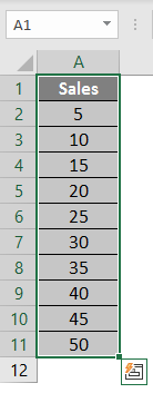
Step 1: Open MS Excel from the start menu >> Go to Sheet1, where the user has kept the data.
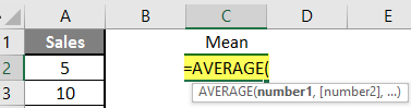
Step 2: Now create headers for Mean where we will calculate the mean of the numbers.
![]()
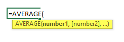
Step 3: Now calculate the mean of the given number by average function>> use the equal sign to calculate >> Write in cell C2 and use average>> “=AVERAGE (“
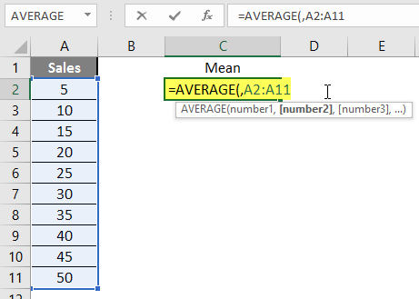
Step 3: Now, it will ask for a number1, which is given in column A >> there are 2 methods to provide input either a user can give one by one or just give the range of data >> select data set from A2 to A11 >> write in cell C2 and use average>> “=AVERAGE (A2: A11) “
Step 4: Now press the enter key >> Mean will be calculated.
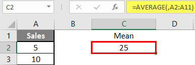
Summary of Example 1: As the user wants to perform the mean calculation for all numbers in MS Excel. Easley everything calculated in the above excel example, and the Mean is 27.5 for sales.
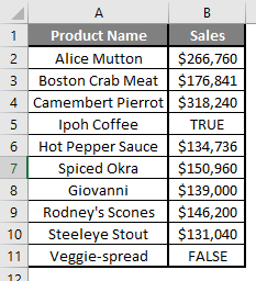
Example #2 – How to Calculate Mean if Text Value Exists in the Data Set
Let’s calculate the Mean if there is some text value in the Excel data set. Let’s assume a user wants to perform the calculation for some sales data set in Excel. But there is some text value also there. So, he wants to use count for all, either its text or number. Let’s see how we can do this with the AVERAGE function. Because in the normal AVERAGE function, it will exclude the text value count.
Step 1: Open MS Excel from the start menu >> Go to Sheet2, where the user has kept the data.
Step 2: Now create headers for Mean where we will calculate the mean of the numbers.
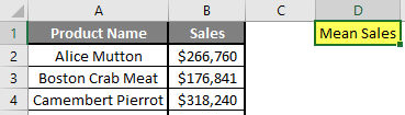
Step 3: Now calculate the mean of the given number by average function>> use the equal sign to calculate >> Write in cell D2 and use AVERAGEA>> “=AVERAGEA (“
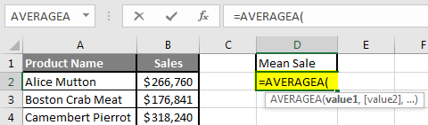
Step 4: Now, it will ask for a number1, which is given in column B >> there is two open to provide input either a user can give one by one or just give the range of data >> select data set from B2 to B11 >> write in D2 Cell and use average>> “=AVERAGEA (D2: D11) “
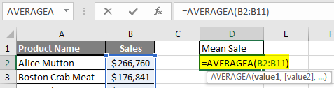
Step 5: Now click on the enter button >> Mean will be calculated.
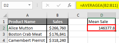
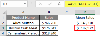
Step 6: Just to compare the AVERAGEA and AVERAGE, in normal average, it will exclude the count for text value so mean will high than the AVERAGE MEAN.
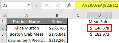
Summary of Example 2: As the user wants to perform the mean calculation for all number in MS Excel. Easley, everything calculated in the above excel example and the Mean is $146377.80 for sales.
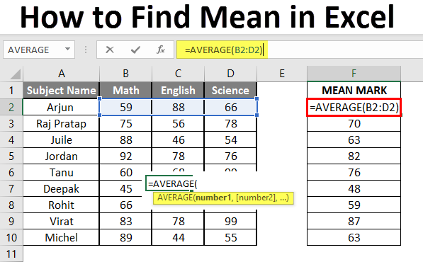
Example #3 – How to Calculate Mean for Different Set of Data
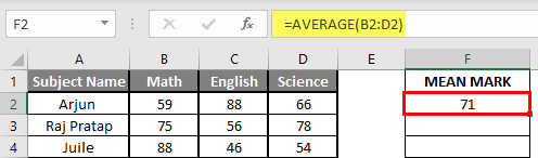
Let’s assume a user wants to perform the calculation for some student’s mark data set in MS Excel. There are ten student marks for Math, English, and Science out of 100. Let’s see How to Find Mean in Excel with the AVERAGE function.
Step 1: Open the MS Excel from the start menu >> Go to Sheet3, where the user kept the data.
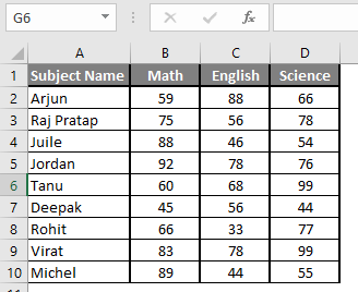
Step 2: Now create headers for Mean where we will calculate the mean of the numbers.
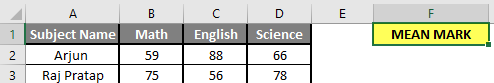
Step 3: Now calculate the mean of the given number by average function>> use the equal sign to calculate >> Write in F2 Cell and use AVERAGE >> “=AVERAGE (“
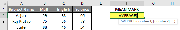
Step 3: Now, it will ask for number1 which is given in B, C, and D column >> there is two open to provide input either a user can give one by one or just give the range of data >> Select data set from B2 to D2 >> Write in F2 Cell and use average >> “=AVERAGE (B2: D2) “
Step 4: Now click on the enter button >> Mean will be calculated.
Step 5: Now click on the F2 cell and drag and apply to another cell in the F column.
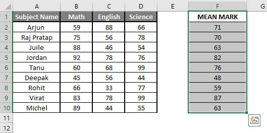
Summary of Example 3: As the user wants to perform the mean calculation for all number in MS Excel. Easley, everything calculated in the above excel example and the Mean is available in the F column.
Things to Remember About How to Find Mean in Excel
- Microsoft Excel’s AVERAGE function used to calculate the Arithmetic Mean of the given input. A user can give 255 input arguments in the function.
- Half the set of a number will be smaller than the mean, and the remaining set will be greater than the mean.
- If a user calculating the normal average, it will exclude the count for a text value, so AVERAGE Mean will bigger than the AVERAGE MEAN.
- Arguments can be number, name, range or cell references that should contain a number.
- If a user wants to calculate the mean with some condition, then use AVERAGEIF or AVERAGEIFS.
Recommended Articles
This is a guide to How to Find Mean in Excel. Here we discuss How to Find Mean along with examples and a downloadable excel template. You may also look at the following articles to learn more –
- FIND Function in Excel
- Excel Find
- Excel Average Formula
- Excel AVERAGE Function
You can use the following formulas to find the mean, median, and mode of a dataset in Excel:
=AVERAGE(A1:A10)

=MEDIAN(A1:A10)

=MODE.MULT(A1:A10)
It’s worth noting that each of these formulas will simply ignore non-numeric or blank values when calculating these metrics for a range of cells in Excel.
The following examples shows how to use these formulas in practice with the following dataset:

Example: Finding the Mean in Excel
The mean represents the average value in a dataset.
The following screenshot shows how to calculate the mean of a dataset in Excel:

The mean turns out to be 19.11.
Example: Finding the Median in Excel
The median represents the middle value in a dataset, when all of the values are arranged from smallest to largest.
The following screenshot shows how to calculate the median of a dataset in Excel:

The median turns out to be 20.
Example: Finding the Mode in Excel
The mode represents the value that occurs most often in a dataset. Note that a dataset can have no mode, one mode, or multiple modes.
The following screenshot shows how to calculate the mode(s) of a dataset in Excel:

The modes turn out to be 7 and 25. Each of these values appears twice in the dataset, which is more often than any other value occurs.
Note: If you use the =MODE() function instead, it will only return the first mode. For this dataset, only the value 7 would be returned. For this reason, it’s always a good idea to use the =MODE.MULT() function in case there happens to be more than one mode in the dataset.
Additional Resources
How to Calculate the Interquartile Range (IQR) in Excel
How to Calculate the Midrange in Excel
How to Calculate Standard Deviation in Excel
Learn quick and simple ways to calculate mean in excel. Read the article to know how.
Excel is a widely popular program which is used to analyse and organize large amounts of data and information. Finding out the mean is one of the most important functions of analyzing data. But what is mean?
The mean is the average number when all of the data is added and divided by the number of data points. Let us know what the mean is, its uses and how to calculate the mean in Excel for your usage.
Uses For Mean in Excel
There are many uses for the mean in Excel. The mean is found by adding up all of the numbers in a set of data and dividing by the number of points that are added together. It tells you the typical value in a given set of information. Some ways you can use the mean in analyzing data:
- To find a standard midpoint for comparing individual data points.
- To determine quotas and key performance indicators (KPIs).
- To compare historical data.
- To guide project management and business strategy.
Specifying Mean Calculation Criteria in Excel
Here are some scenarios where you will need to use more specific mean formulas to know if the information should be included in the calculation:
- You want to include cells with values of zero or text. If you want to include cells with any data in your calculations, you would use the formula AVERAGEA.
- You want to include cells that meet specific criteria. If you only want to find the mean of certain information that is based on one criterion, you would use the formula AVERAGEIF. You might use this if you are trying to find the mean of every cell that doesn’t meet a quota or the mean salary over a certain pay grade.
- You want to include cells that meet several specific criteria. If you are trying to find the mean of information that meets two or more requirements, you would use the formula AVERAGEIFS. You might use this if you are trying to find the mean of cells that are within a certain number range.
There are many ways to calculate the mean of a data set. It depends on what you are trying to find in the data. Here is how to calculate the mean of an entire data set:
Example #1 – How to Calculate Mean in Excel In the Basic Way
Step 1: Open MS Excel from the start menu >> Go to Sheet1, where the user has kept the data.

Step 2: Create headers for the Mean where we will calculate the mean of the numbers.

Step 3: Calculate the mean of the given number by average function>> use the equal sign to calculate >> Write in cell C2 and use average>> “=AVERAGE (“

Step 4: Now, it will ask for a number1, which is given in column A >> there are 2 methods to provide input either a user can give one by one or just give the range of data >> select data set from A2 to A11 >> write in cell C2 and use average>> “=AVERAGE (A2: A11) “

Step 5: Press the enter key >> Mean will be calculated.

Example #2 – How to Calculate Mean In Excel if Text Value Exists in the Data Set
Let’s calculate the Mean if there is some text value in the Excel data set.
Step 1: Open MS Excel from the start menu >> Go to Sheet2, where the user has kept the data.

Step 2: Create headers for the Mean where we will calculate the mean of the numbers.

Step 3: Calculate the mean of the given number by average function>> use the equal sign to calculate >> Write in cell D2 and use AVERAGEA>> “=AVERAGEA (“

Step 4: It will ask for a number1, which is given in column B >> there is two open to provide input either a user can give one by one or just give the range of data >> select data set from B2 to B11 >> write in D2 Cell and use average>> “=AVERAGEA (D2: D11) “

Step 5: Click on the enter button >> Mean will be calculated.

Step 6: Just to compare the AVERAGEA and AVERAGE, in normal average, it will exclude the count for text value so the mean will high than the AVERAGE MEAN.


Example #3 – How to Calculate Mean In Excel for Different Sets of Data
Let’s assume a user wants to perform the calculation for a student’s mark data set in MS Excel. There are ten student marks for Math, English, and Science out of 100. Let’s see How to Find Mean in Excel with the AVERAGE function.
Step 1: Open MS Excel from the start menu >> Go to Sheet3, where the user kept the data.

Step 2: Now create headers for the Mean where we will calculate the mean of the numbers.

Step 3: Calculate the mean of the given number by average function>> use the equal sign to calculate >> Write in F2 Cell and use AVERAGE >> “=AVERAGE (“

Step 4: Now, it will ask for number 1 which is given in B, C, and D column >> there are two open to provide input either a user can give one by one or just give the range of data >> Select data set from B2 to D2 >> Write in F2 Cell and use average >> “=AVERAGE (B2: D2) “

Step 5: Now click on the enter button >> Mean will be calculated.

Step 6: Now click on the F2 cell and drag and apply to another cell in the F column.

Step 1: Click an empty cell. Step 2: Type “=AVERAGE(A1:A10)” where A1:A10 is the location of your data set. For example, if you want to find a mean for a data set in cells A1 to A99, type “A1:A99”. Step 3: Press “Enter” to display the mean.
Contents
- 1 How do I calculate mean in Excel?
- 2 What is the mean function in Excel?
- 3 How do you calculate mean?
- 4 How do you find the mean of a set of data?
- 5 How do you find the mean median and mode?
- 6 How do you find the mean of two means?
- 7 Why do you calculate a mean?
- 8 Why do we calculate the mean?
- 9 How do you find the mad of a set of data?
- 10 How do you find the mean of a big data set?
- 11 Is mean same as average?
- 12 How do you calculate mean with examples?
- 13 When to use median vs mean?
- 14 How do you find the mean and standard deviation of grouped data in Excel?
- 15 How do you find the mean of the distribution of means?
- 16 How do you find the mean of two sets of data?
- 17 How do you find the mean point?
- 18 How do you calculate mean time?
- 19 Does the mean represent the center of the data?
How do I calculate mean in Excel?
To find the mean in Excel, you start by typing the syntax =AVERAGE or select AVERAGE from the formula dropdown menu. Then, you select which cells will be included in the calculation. For example: Say you will be calculating the mean for column A, rows two through 20. Your formula will look like this: =AVERAGE(A2:A20).
What is the mean function in Excel?
The mean or the statistical mean is essentially means average value and can be calculated by adding data points in a setand then dividing the total, by the number of points. Excel’s AVERAGE function does exactly this: sum all the values and divides the total by the count of numbers.
How do you calculate mean?
Remember, the mean is calculated by adding the scores together and then dividing by the number of scores you added. In this case, the mean would be 2 + 4 (add the two middle numbers), which equals 6. Then, you take 6 and divide it by 2 (the total number of scores you added together), which equals 3.
How do you find the mean of a set of data?
The mean (average) of a data set is found by adding all numbers in the data set and then dividing by the number of values in the set.
How do you find the mean median and mode?
For example, take this list of numbers: 10, 10, 20, 40, 70.
- The mean (informally, the “average“) is found by adding all of the numbers together and dividing by the number of items in the set: 10 + 10 + 20 + 40 + 70 / 5 = 30.
- The median is found by ordering the set from lowest to highest and finding the exact middle.
How do you find the mean of two means?
A combined mean is a mean of two or more separate groups, and is found by : Calculating the mean of each group, Combining the results.
To calculate the combined mean:
- Multiply column 2 and column 3 for each row,
- Add up the results from Step 1,
- Divide the sum from Step 2 by the sum of column 2.
Why do you calculate a mean?
The mean is used to summarize a data set. It is a measure of the center of a data set.
Why do we calculate the mean?
The mean is essentially a model of your data set.An important property of the mean is that it includes every value in your data set as part of the calculation. In addition, the mean is the only measure of central tendency where the sum of the deviations of each value from the mean is always zero.
How do you find the mad of a set of data?
Calculate Mean Absolute Deviation (M.A.D)
- To find the mean absolute deviation of the data, start by finding the mean of the data set.
- Find the sum of the data values, and divide the sum by the number of data values.
- Find the absolute value of the difference between each data value and the mean: |data value – mean|.
How do you find the mean of a big data set?
How to Find the Mean
- Add up all data values to get the sum.
- Count the number of values in your data set.
- Divide the sum by the count.
Is mean same as average?
Average, also called the arithmetic mean, is the sum of all the values divided by the number of values. Whereas, mean is the average in the given data. In statistics, the mean is equal to the total number of observations divided by the number of observations.
How do you calculate mean with examples?
Mean: The “average” number; found by adding all data points and dividing by the number of data points. Example: The mean of 4, 1, and 7 is ( 4 + 1 + 7 ) / 3 = 12 / 3 = 4 (4+1+7)/3 = 12/3 = 4 (4+1+7)/3=12/3=4left parenthesis, 4, plus, 1, plus, 7, right parenthesis, slash, 3, equals, 12, slash, 3, equals, 4.
When to use median vs mean?
Mean is the most frequently used measure of central tendency and generally considered the best measure of it. However, there are some situations where either median or mode are preferred. Median is the preferred measure of central tendency when: There are a few extreme scores in the distribution of the data.
How do you find the mean and standard deviation of grouped data in Excel?
But first, let us have some sample data to work on:
- Calculate the mean (average)
- For each number, subtract the mean and square the result.
- Add up squared differences.
- Divide the total squared differences by the count of values.
- Take the square root.
- Excel STDEV function.
- Excel STDEV.
- Excel STDEVA function.
How do you find the mean of the distribution of means?
Calculate the mean of each sample by taking the sum of the sample values and dividing by the number of values in the sample. For example, the mean of the sample 9, 4 and 5 is (9 + 4 + 5) / 3 = 6.
How do you find the mean of two sets of data?
How to Find the Mean: Overview. To find the arithmetic mean of a data set, all you need to do is add up all the numbers in the data set and then divide the sum by the total number of values.
How do you find the mean point?
To find the mean, add up all the numbers in the data set. Then, divide by how many numbers there are.
How do you calculate mean time?
Mean time to failure is an arithmetic average, so you calculate it by adding up the total operating time of the products you’re assessing and dividing that total by the number of devices. For example: Let’s say you’re figuring out the MTTF of light bulbs.
Does the mean represent the center of the data?
the mean represents the center of a numerical data set. to find the mean, sum the data values & then divide by the number of values in the data set.
The mean (or average) of a dataset is one of the most common ways to analyze data. Let’s learn how to find a mean in Excel.
The mean (or average) of a dataset is one of the most common ways to analyze data. Excel makes it easy. Let’s learn how to find a mean in Excel.
How to Find the Mean in Excel (With AutoSum)
Excel offers at least two quick ways to find the mean. The fastest way comes if your data is in a row or column.
Consider a column of data like this. It has nine unique numbers, and you want to quickly find the average.

To do that, click into the empty cell immediately below the last number. Then, go to the Home tab on Excel’s ribbon. You’ll see the AutoSum button in the Editing group.
Click on the dropdown arrow immediately to the right of AutoSum (if you click AutoSum, the numbers will be added, not averaged).

You’ll see a few options on the dropdown, the second one being Average. Click it, and then highlight your data. Excel will automatically average it for you.

If you’re working with a row of data, the process is identical. Simply click into the empty cell to the immediate right of your last number, and repeat the AutoSum steps.
How to Find the Mean from Multiple Rows and Columns
Imagine now that you have multiple rows or columns, and need to find the mean of numbers within them. This is almost as easy.
Suppose you need to find the average of the numbers in rows 1, 2, 3, and 4. Begin by clicking into an empty cell. Type = to start a formula, then AVERAGE(.
Click and drag to select your data set: in this case, A1:D4. Close the ). Your formula should read:
=AVERAGE(A1:D4)

Hit Enter on your keyboard, and Excel will calculate the average of all the data.
As you can see, Excel makes finding the mean simple. Use these techniques next time you’re analyzing any dataset.
Finding the mean (or average) of a set of values is used in many contexts, including business, finance, and research. Microsoft Excel can find the mean for any set of values you choose as input.
So, how do you find mean in Excel? To find mean in Excel, use the “AVERAGE” function. The input to the average function is a range of cells (you can enter one or more cells, rows, or columns, separating inputs with a comma). For example, the mean of the values in cells A1 to A20 would be given by the formula “=AVERAGE(A1:A20)”.
Of course, when dealing with the mean, remember that population mean takes into account every person or item in the entire group, while sample mean only uses a subset of the group.
In this article, we’ll talk about finding mean in Excel, including how to do it, alternative methods, and when you might use it. We’ll also look at some other types of mean, including geometric mean, harmonic mean, and weighted averages.
Let’s get started.
How To Find Mean In Excel (The Average Function In Excel)
The easiest way to find the mean (also called arithmetic mean) in Excel is to use the “AVERAGE” function. This function can take one or more inputs, separated by commas.
Each input is one or more cells – an input can be:
- a single cell (for example, “A1” would be a single cell)
- a row (for example, “A1:J1” would be a row consisting of 10 cells)
- a column (for example, “A1:A8” would be a column consisting of 8 cells)
- a block of cells (for example, “A1:J8” would be a block of cells consisting of 8 rows and 10 columns, for a total of 8*10 = 80 cells)
- a named range (for example “my_values”, which could denote any set of cells you choose, including an individual cell, a row, a column, or a block of cells)
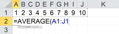
For example, the mean of the values in cells A1 to J1 (a row of 10 cells) would be given by the formula
- =AVERAGE(A1:J1)
You can see an example of this illustrated below.
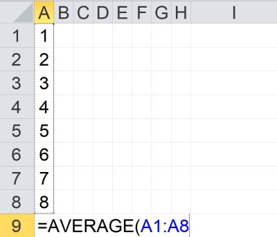
The mean of the values in cells A1 to A8 (a column of 8 cells) would be given by the formula
- =AVERAGE(A1:A8)
You can see an example of this illustrated below.
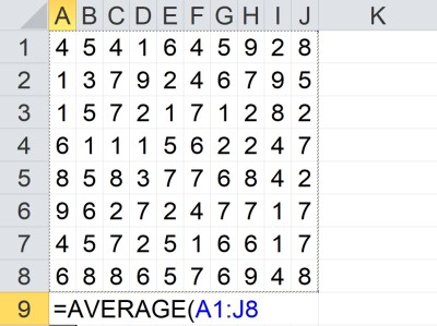
The mean of the values in cells A1 to J8 (a block of 80 cells) would be given by the formula
- =AVERAGE(A1:J8)
You can see an example of this illustrated below.
The mean of the value in cells A1 to A5 and C1 to C5 would be given by the formula
- =AVERAGE(A1:A5, C1:C5)
You can see an example of this illustrated below.
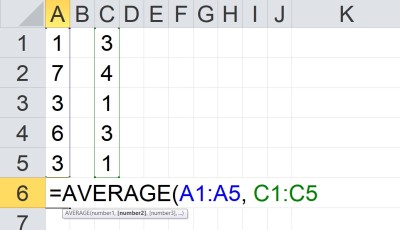
Note that the two inputs (A1:A5 and C1:C5) are separated by a comma. Each input has a total of 5 cells, for a total of 10 cells as input.
Also note that we can take the average of any combination of cells, rows, columns, and blocks.
Alternative To Average In Excel
One alternative to the AVERAGE function in Excel is to combine the SUM and COUNT functions, along with division (denoted by the “/” symbol).
Remember that the mean (average or arithmetic mean) for a set of n values {x1, x2, … , xn} is given by the formula:
- Mean = (x1 + x2 + … + xn) / n
or, as an Excel formula for n = 10:
- =SUM(A1:A10) / COUNT(A1:A10)
The above formula will return the same result as
- =AVERAGE(A1:A10)
The alternative method is useful in some cases when you might like to show the sum, the count, and the mean that comes from dividing the sum by the count.
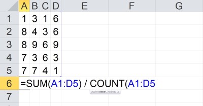
Example: Alternative To Average In Excel
Let’s say we want to find the mean of the set of values in the cells A1:D5 in Excel. Instead of using the AVERAGE function, we can divide the SUM function by the COUNT function as follows:
- =SUM(A1:D5) / COUNT(A1:D5)
You can see an example of this illustrated below.
Note that you can also use a named range to make it easier to change inputs later. For example, if you create a named range called “my_values” and define it to be cells A1:D5, you can use the formula:
- =SUM(my_values) / COUNT(my_values)
You can see an example of this illustrated below.
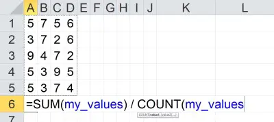
If you change the definition of the named range my_values to cells A1:E5, the sum and count will be updated to reflect the new input range (as will the average).
Is Average The Same As Mean In Excel? (Difference Between Mean & Average)
In Excel, average is the same as mean. That is, there is no difference between mean and average in Excel.
However, there are different types of means that we can use. For example, there is geometric mean and also harmonic mean (we will look at both of these later).
There is also a weighted average, which assigns different weight to each value. The arithmetic mean (or mean, or average) assigns equal weight to each value.
When To Use Average In Excel
The average (or mean) is a measure of center in a data set. So, you might use an average in Excel to tell you where the center of a data set lies.

(You can learn more about uses of mean in this article).
You can also use median or mode as alternative measures of center for a data set. You can learn more about the differences between mean and median here.
Another way to use average in Excel is to track the performance of a group or to compare multiple groups, based on a data set from each group. For example, you could track the average revenue per month, quarter, or year for one or more groups of salespeople at a company.
How To Calculate Geometric Mean In Excel
Remember that the geometric mean for a set of n values {x1, x2, … , xn} is given by the formula:
- Geometric Mean = n√(x1*x2*…*xn)
In other words, the geometric mean of a set of n values is the principal nth root of the product of those n numbers.
The easiest way to find the geometric mean in Excel is to use the “GEOMEAN” function. This function can take one or more inputs, separated by commas.
Each input is one or more cells – an input can be:
- a single cell (for example, “A1” would be a single cell)
- a row (for example, “A1:J1” would be a row consisting of 10 cells)
- a column (for example, “A1:A8” would be a column consisting of 8 cells)
- a block of cells (for example, “A1:J8” would be a block of cells consisting of 8 rows and 10 columns, for a total of 8*10 = 80 cells)
- a named range (for example “my_values”, which could denote any set of cells you choose, including an individual cell, a row, a column, or a block of cells)
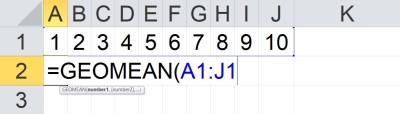
For example, the geometric mean of the values in cells A1 to J1 (a row of 10 cells) would be given by the formula
- =GEOMEAN(A1:J1)
You can see an example of this illustrated below.
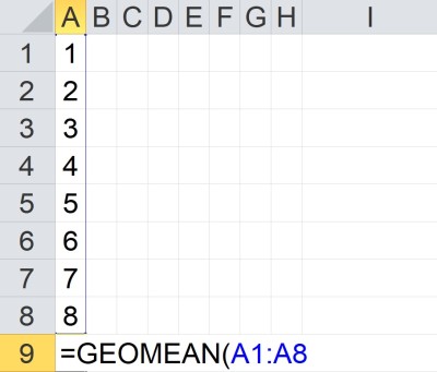
The geometric mean of the values in cells A1 to A8 (a column of 8 cells) would be given by the formula
- =GEOMEAN(A1:A8)
You can see an example of this illustrated below.
How To Calculate Harmonic Mean In Excel
Remember that the harmonic mean for a set of n values {x1, x2, … , xn} is given by the formula:
- Harmonic Mean = n / (x1-1 + x2-1 … + xn-1)
In other words, to find the harmonic mean of a set of n values, we take these steps:
- Step 1: Find the reciprocal (inverse) of each of the n values in the set of numbers (so x1-1 = 1/x1, x2-1 = 1/x2, etc.)
- Step 2: take the sum of the n reciprocals from Step 1 (calculate x1-1 + x2-1 … + xn-1).
- Step 3: take the reciprocal of the sum from Step 2 (calculate 1 / (x1-1 + x2-1 … + xn-1)).
- Step 4: multiply the result of Step 3 by n (calculate n / (x1-1 + x2-1 … + xn-1)).
The easiest way to find the geometric mean in Excel is to use the “HARMEAN” function. This function can take one or more inputs, separated by commas.
Each input is one or more cells – an input can be:
- a single cell (for example, “A1” would be a single cell)
- a row (for example, “A1:J1” would be a row consisting of 10 cells)
- a column (for example, “A1:A8” would be a column consisting of 8 cells)
- a block of cells (for example, “A1:J8” would be a block of cells consisting of 8 rows and 10 columns, for a total of 8*10 = 80 cells)
- a named range (for example “my_values”, which could denote any set of cells you choose, including an individual cell, a row, a column, or a block of cells)
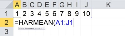
For example, the harmonic mean of the values in cells A1 to J1 (a row of 10 cells) would be given by the formula
- =HARMEAN(A1:J1)
You can see an example of this illustrated below.
The harmonic mean of the values in cells A1 to A8 (a column of 8 cells) would be given by the formula
- =HARMEAN(A1:A8)
You can see an example of this illustrated below.

How To Calculate Weighted Average In Excel (Weighted Mean)
The easiest way to calculate weighted average (weighted mean) in Excel is to use the SUMPRODUCT formula. The first input is the set of values, and the second input is the set of weights.
Note that the values and weights should correspond. If they do not, you will be assigning the wrong weights to each value.
Also, the weights should add up to 1 (100%).
Example: Weighted Average In Excel
Let’s say we want to take a weighted average of 5 values in Excel. The table below gives the values and the weights:
| Values | Weights |
|---|---|
| 2 | 0.1 |
| 5 | 0.15 |
| 7 | 0.25 |
| 11 | 0.3 |
| 15 | 0.2 |
In Excel, we would put the numbers from column 1 in the table (values) into cells A1:A5. Then, we would put the numbers from column 2 in the table (weights) into cells B1:B5.

Finally, we would use the SUMPRODUCT formula to multiply each value in the first column by its corresponding weight in the second column, and then add up the products.
The formula would be:
- =SUMPRODUCT(A1:A5, B1:B5)
You can see a picture of this below.

Conclusion
Now you know how to find mean in Excel, as well as an alternative method to find the mean in Excel and how to use named ranges. You also know how to find other types of means and weighted averages in Excel.
You can learn more about what mean tells you about data (along with lots of examples) here.
You can learn how to calculate median in Excel here.
You can learn how to calculate the mode in Excel here.
You can learn about the differences between mean and standard deviation here.
Calculating the mean of numbers is one of staples of statistical analysis processes. In this article, we’re going to show you how to calculate mean in Excel using the AVERAGE formula.
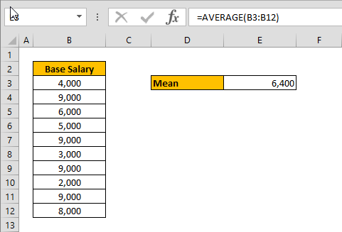
Syntax
=AVERAGE( array of numbers )
Steps
- Begin by creating the formula =AVERAGE(
- Select your data range that contains the values (i.e. B3:B12)
- Finish the formula with ) and press the Enter key.
How to find the mean in Excel
The mean or the statistical mean is essentially means average value and can be calculated by adding data points in a setand then dividing the total, by the number of points. Excel’s AVERAGE function does exactly this: sum all the values and divides the total by the count of numbers.
The AVERAGE function can also be configured to ignore empty cells and cells that do not include any numbers. If you want to include empty or invalid values in calculations as zeroes, use the AVERAGEA function. The AVERAGEA function works exactly the same with the AVERAGE.
=AVERAGEA( array of numbers )
For more information about AVERAGE formula please see our related article.
![]()
Finding the mean comes in handy when processing and analyzing all kinds of data. With Microsoft Excel’s AVERAGE function, you can quickly and easily find the mean for your values. We’ll show you how to use the function in your spreadsheets.
How Microsoft Excel Calculates the Mean
By definition, the mean for a data set is the sum of all the values in the set divided by the count of those values.
For example, if your data set contains 1, 2, 3, 4, and 5, the mean for this data set is 3. You can find it with the following formula.
(1+2+3+4+5)/5
You could type out formulas like that yourself, but Excel’s AVERAGE function helps you perform this calculation with ease.
Find the Mean Using a Function in Microsoft Excel
In our example, we’ll find the mean for the values in the “Score” column, and display the answer in the C9 cell.
We’ll start by clicking the C9 cell where we want to display the resulting mean.

In the C9 cell, we’ll type the following function. This function finds the mean for the values in all the cells between C2 and C6 (both these cells included).
=AVERAGE(C2:C6)
Press Enter and the result will appear in the C9 cell.
You can use the AVERAGE function to find the mean for any values in your spreadsheet. Enjoy!
Getting the mean will come in handy if you ever need Excel to calculate uncertainty.
RELATED: How to Get Microsoft Excel to Calculate Uncertainty
READ NEXT
- › How to Calculate Average in Microsoft Excel
- › How to Combine Data From Spreadsheets in Microsoft Excel
- › How to Manage Conditional Formatting Rules in Microsoft Excel
- › How to Calculate the Median in Microsoft Excel
- › HoloLens Now Has Windows 11 and Incredible 3D Ink Features
- › The New NVIDIA GeForce RTX 4070 Is Like an RTX 3080 for $599
- › How to Adjust and Change Discord Fonts
- › This New Google TV Streaming Device Costs Just $20
How-To Geek is where you turn when you want experts to explain technology. Since we launched in 2006, our articles have been read billions of times. Want to know more?