

Use the Find and Replace features in Excel to search for something in your workbook, such as a particular number or text string. You can either locate the search item for reference, or you can replace it with something else. You can include wildcard characters such as question marks, tildes, and asterisks, or numbers in your search terms. You can search by rows and columns, search within comments or values, and search within worksheets or entire workbooks.

Find
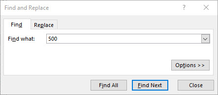
To find something, press Ctrl+F, or go to Home > Editing > Find & Select > Find.
Note: In the following example, we’ve clicked the Options >> button to show the entire Find dialog. By default, it will display with Options hidden.

-
In the Find what: box, type the text or numbers you want to find, or click the arrow in the Find what: box, and then select a recent search item from the list.
Tips: You can use wildcard characters — question mark (?), asterisk (*), tilde (~) — in your search criteria.
-
Use the question mark (?) to find any single character — for example, s?t finds «sat» and «set».
-
Use the asterisk (*) to find any number of characters — for example, s*d finds «sad» and «started».
-
Use the tilde (~) followed by ?, *, or ~ to find question marks, asterisks, or other tilde characters — for example, fy91~? finds «fy91?».
-
-
Click Find All or Find Next to run your search.
Tip: When you click Find All, every occurrence of the criteria that you are searching for will be listed, and clicking a specific occurrence in the list will select its cell. You can sort the results of a Find All search by clicking a column heading.
-
Click Options>> to further define your search if needed:
-
Within: To search for data in a worksheet or in an entire workbook, select Sheet or Workbook.
-
Search: You can choose to search either By Rows (default), or By Columns.
-
Look in: To search for data with specific details, in the box, click Formulas, Values, Notes, or Comments.
Note: Formulas, Values, Notes and Comments are only available on the Find tab; only Formulas are available on the Replace tab.
-
Match case — Check this if you want to search for case-sensitive data.
-
Match entire cell contents — Check this if you want to search for cells that contain just the characters that you typed in the Find what: box.
-
-
If you want to search for text or numbers with specific formatting, click Format, and then make your selections in the Find Format dialog box.
Tip: If you want to find cells that just match a specific format, you can delete any criteria in the Find what box, and then select a specific cell format as an example. Click the arrow next to Format, click Choose Format From Cell, and then click the cell that has the formatting that you want to search for.
Replace
To replace text or numbers, press Ctrl+H, or go to Home > Editing > Find & Select > Replace.
Note: In the following example, we’ve clicked the Options >> button to show the entire Find dialog. By default, it will display with Options hidden.

-
In the Find what: box, type the text or numbers you want to find, or click the arrow in the Find what: box, and then select a recent search item from the list.
Tips: You can use wildcard characters — question mark (?), asterisk (*), tilde (~) — in your search criteria.
-
Use the question mark (?) to find any single character — for example, s?t finds «sat» and «set».
-
Use the asterisk (*) to find any number of characters — for example, s*d finds «sad» and «started».
-
Use the tilde (~) followed by ?, *, or ~ to find question marks, asterisks, or other tilde characters — for example, fy91~? finds «fy91?».
-
-
In the Replace with: box, enter the text or numbers you want to use to replace the search text.
-
Click Replace All or Replace.
Tip: When you click Replace All, every occurrence of the criteria that you are searching for will be replaced, while Replace will update one occurrence at a time.
-
Click Options>> to further define your search if needed:
-
Within: To search for data in a worksheet or in an entire workbook, select Sheet or Workbook.
-
Search: You can choose to search either By Rows (default), or By Columns.
-
Look in: To search for data with specific details, in the box, click Formulas, Values, Notes, or Comments.
Note: Formulas, Values, Notes and Comments are only available on the Find tab; only Formulas are available on the Replace tab.
-
Match case — Check this if you want to search for case-sensitive data.
-
Match entire cell contents — Check this if you want to search for cells that contain just the characters that you typed in the Find what: box.
-
-
If you want to search for text or numbers with specific formatting, click Format, and then make your selections in the Find Format dialog box.
Tip: If you want to find cells that just match a specific format, you can delete any criteria in the Find what box, and then select a specific cell format as an example. Click the arrow next to Format, click Choose Format From Cell, and then click the cell that has the formatting that you want to search for.
There are two distinct methods for finding or replacing text or numbers on the Mac. The first is to use the Find & Replace dialog. The second is to use the Search bar in the ribbon.
Find & Replace dialog
Search bar and options

-
Press Ctrl+F or go to Home > Find & Select > Find.
-
In Find what: type the text or numbers you want to find.
-
Select Find Next to run your search.
-
You can further define your search:
-
Within: To search for data in a worksheet or in an entire workbook, select Sheet or Workbook.
-
Search: You can choose to search either By Rows (default), or By Columns.
-
Look in: To search for data with specific details, in the box, click Formulas, Values, Notes, or Comments.
-
Match case — Check this if you want to search for case-sensitive data.
-
Match entire cell contents — Check this if you want to search for cells that contain just the characters that you typed in the Find what: box.
-
Tips: You can use wildcard characters — question mark (?), asterisk (*), tilde (~) — in your search criteria.
-
Use the question mark (?) to find any single character — for example, s?t finds «sat» and «set».
-
Use the asterisk (*) to find any number of characters — for example, s*d finds «sad» and «started».
-
Use the tilde (~) followed by ?, *, or ~ to find question marks, asterisks, or other tilde characters — for example, fy91~? finds «fy91?».

-
Press Ctrl+F or go to Home > Find & Select > Find.
-
In Find what: type the text or numbers you want to find.
-
Select Find All to run your search for all occurrences.

Note: The dialog box expands to show a list of all the cells that contain the search term, and the total number of cells in which it appears.
-
Select any item in the list to highlight the corresponding cell in your worksheet.
Note: You can edit the contents of the highlighted cell.

-
Press Ctrl+H or go to Home > Find & Select > Replace.
-
In Find what, type the text or numbers you want to find.
-
You can further define your search:
-
Within: To search for data in a worksheet or in an entire workbook, select Sheet or Workbook.
-
Search: You can choose to search either By Rows (default), or By Columns.
-
Match case — Check this if you want to search for case-sensitive data.
-
Match entire cell contents — Check this if you want to search for cells that contain just the characters that you typed in the Find what: box.
Tips: You can use wildcard characters — question mark (?), asterisk (*), tilde (~) — in your search criteria.
-
Use the question mark (?) to find any single character — for example, s?t finds «sat» and «set».
-
Use the asterisk (*) to find any number of characters — for example, s*d finds «sad» and «started».
-
Use the tilde (~) followed by ?, *, or ~ to find question marks, asterisks, or other tilde characters — for example, fy91~? finds «fy91?».
-
-
-
In the Replace with box, enter the text or numbers you want to use to replace the search text.
-
Select Replace or Replace All.
Tips:
-
When you select Replace All, every occurrence of the criteria that you are searching for is replaced.
-
When you select Replace, you can replace one instance at a time by selecting Next to highlight the next instance.
-
-
Select any cell to search the entire sheet or select a specific range of cells to search.
-
Press Command + F or select the magnifying glass to expand the Search bar and type the text or number you want to find in the search field.
Tips: You can use wildcard characters — question mark (?), asterisk (*), tilde (~) — in your search criteria.
-
Use the question mark (?) to find any single character — for example, s?t finds «sat» and «set».
-
Use the asterisk (*) to find any number of characters — for example, s*d finds «sad» and «started».
-
Use the tilde (~) followed by ?, *, or ~ to find question marks, asterisks, or other tilde characters — for example, fy91~? finds «fy91?».
-
-
Press return.
Notes:
-
To find the next instance of the item you are searching for, press return again or use the Find dialog box and select Find Next.
-
To specify additional search options, select the magnifying glass and select Search in Sheet or Search in Workbook. You can also select the Advanced option, which launches the Find dialog.
Tip: You can cancel a search in progress by pressing ESC.
-
Find
To find something, press Ctrl+F, or go to Home > Editing > Find & Select > Find.
Note: In the following example, we’ve clicked > Search Options to show the entire Find dialog. By default, it will display with Search Options hidden.

-
In the Find what: box, type the text or numbers you want to find.
Tips: You can use wildcard characters — question mark (?), asterisk (*), tilde (~) — in your search criteria.
-
Use the question mark (?) to find any single character — for example, s?t finds «sat» and «set».
-
Use the asterisk (*) to find any number of characters — for example, s*d finds «sad» and «started».
-
Use the tilde (~) followed by ?, *, or ~ to find question marks, asterisks, or other tilde characters — for example, fy91~? finds «fy91?».
-
-
Click Find Next or Find All to run your search.
Tip: When you click Find All, every occurrence of the criteria that you are searching for will be listed, and clicking a specific occurrence in the list will select its cell. You can sort the results of a Find All search by clicking a column heading.
-
Click > Search Options to further define your search if needed:
-
Within: To search for data within a certain selection, choose Selection. To search for data in a worksheet or in an entire workbook, select Sheet or Workbook.
-
Direction: You can choose to search either Down (default), or Up.
-
Match case — Check this if you want to search for case-sensitive data.
-
Match entire cell contents — Check this if you want to search for cells that contain just the characters that you typed in the Find what box.
-
Replace
To replace text or numbers, press Ctrl+H, or go to Home > Editing > Find & Select > Replace.
Note: In the following example, we’ve clicked > Search Options to show the entire Find dialog. By default, it will display with Search Options hidden.

-
In the Find what: box, type the text or numbers you want to find.
Tips: You can use wildcard characters — question mark (?), asterisk (*), tilde (~) — in your search criteria.
-
Use the question mark (?) to find any single character — for example, s?t finds «sat» and «set».
-
Use the asterisk (*) to find any number of characters — for example, s*d finds «sad» and «started».
-
Use the tilde (~) followed by ?, *, or ~ to find question marks, asterisks, or other tilde characters — for example, fy91~? finds «fy91?».
-
-
In the Replace with: box, enter the text or numbers you want to use to replace the search text.
-
Click Replace or Replace All.
Tip: When you click Replace All, every occurrence of the criteria that you are searching for will be replaced, while Replace will update one occurrence at a time.
-
Click > Search Options to further define your search if needed:
-
Within: To search for data within a certain selection, choose Selection. To search for data in a worksheet or in an entire workbook, select Sheet or Workbook.
-
Direction: You can choose to search either Down (default), or Up.
-
Match case — Check this if you want to search for case-sensitive data.
-
Match entire cell contents — Check this if you want to search for cells that contain just the characters that you typed in the Find what box.
-
Need more help?
You can always ask an expert in the Excel Tech Community or get support in the Answers community.
Recommended articles
Merge and unmerge cells
REPLACE, REPLACEB functions
Apply data validation to cells
Return to Excel Formulas List
Download Example Workbook
Download the example workbook
This tutorial will demonstrate how to find a number in a column or workbook in Excel and Google Sheets.
Find a Number in a Column
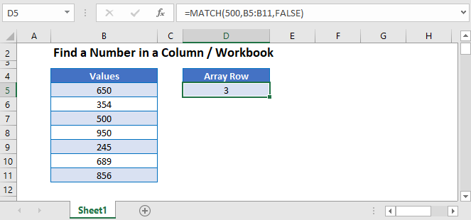
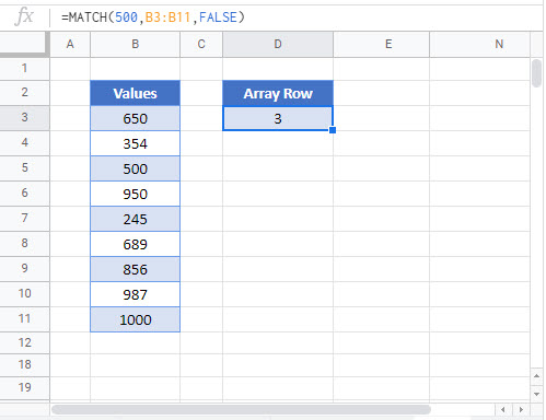
The MATCH Function is useful when you want to find a number within a array of values.
This example will find 500 in column B.
=MATCH(500,B3:B11, 0)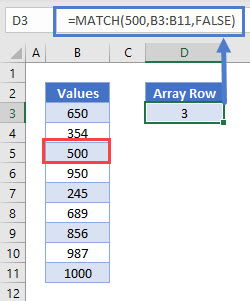
The position of 500 is the 3rd value in the range and returns 3.
Find Row Number of Value Using ROW, INDEX and MATCH Functions
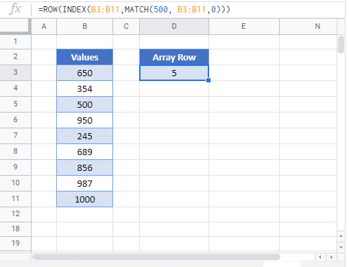
To find the row number of the value found, we can add the ROW and INDEX functions to the MATCH Function.
=ROW(INDEX(B3:B11,MATCH(987,B3:B11,0)))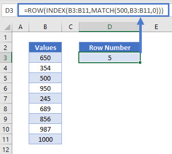
ROW and INDEX Functions
The MATCH Function returns 3 as we have seen from the previous example. The INDEX Function will then return the cell reference or value of the array position returned by the MATCH Function. The ROW function will then return the row of that cell reference.
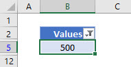
Filter in Excel
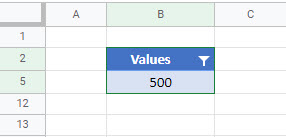
We can find a specific number in an array of data by using a Filter in Excel.
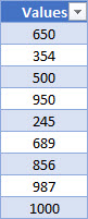
- Click in the Range you want to filter ex B3:B10.
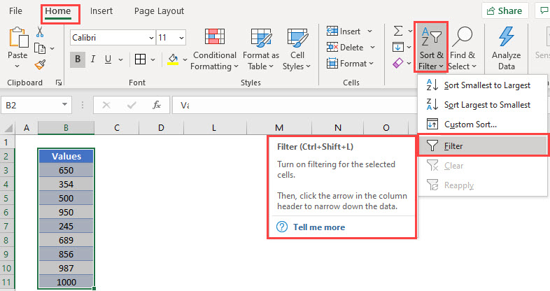
- In the Ribbon, select Home > Editing > Sort & Filter > Filter.
- A drop-down list will be added to the first row in your selected range.
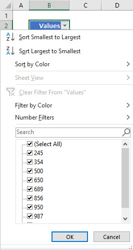
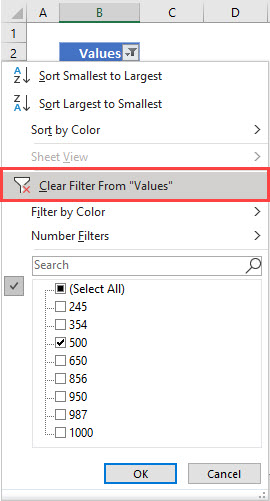
- Click on the drop-down list to get a list of available options.
- Type 500 in the search bar.
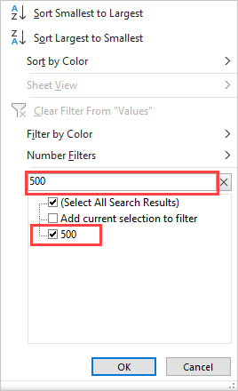
- Click OK.
- If your range has more than one value of 500, then both would show.
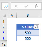
- The rows that do not contain the required values are hidden, and the visible row headers are shown in BLUE.
- To clear the filter, click on the drop-down and then click Clear Filter From “Values”.
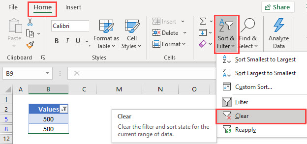
To remove the filter entirely from the Range, select Home > Editing > Sort & Filter > Clear in the Ribbon.
Find Number in Workbook or Worksheet using FIND in Excel
We can look for values in Excel using the FIND functionality.
- In your workbook, press Ctrl+F on the keyboard.
OR
In the Ribbon, select Home > Editing > Find & Select.
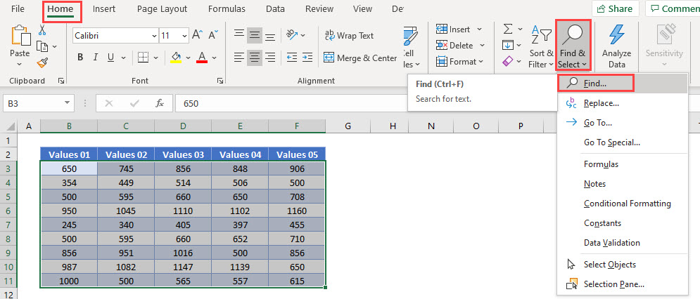
- Type in the value you wish to find.
- Click Find Next.
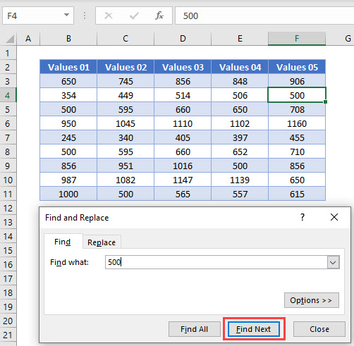
- Continue to click Find Next to move through all the available values in the Worksheet.
- Click Find All to find all the instances of the value in the worksheet.
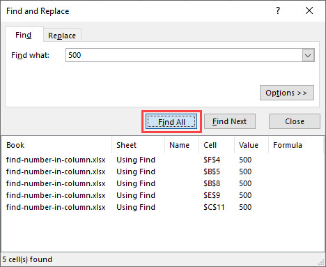
Click Options.
- Amend the Within from Sheet to Workbook and click Find All
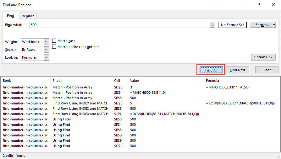
- All the matching values will appear in the results shown.
Find a Number – MATCH Function in Google Sheets
The MATCH Function works the same in Google Sheets as it does in Excel.
Find Row Number of Value Using ROW, INDEX and MATCH Functions in Google Sheets
The ROW, INDEX and MATCH Functions works the same in Google Sheets as it does in Excel.
Filter in Google Sheets
We can find a specific number in an array of data by using Filter in Google Sheets.
- Click in the Range you want to filter ex B3:B10.
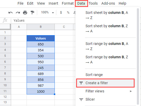
- In the Menu, select Data > Create a filter
- In the Search bar, type in the value you wish to filter on.
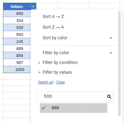
- Click OK.
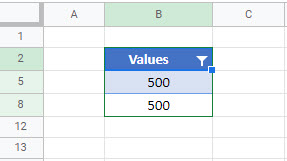
- If your range has more than one value of 500, then both would show.
- The rows that do not contain the required values are hidden.
- To clear the filter, click on the drop-down, click Select All” and then click
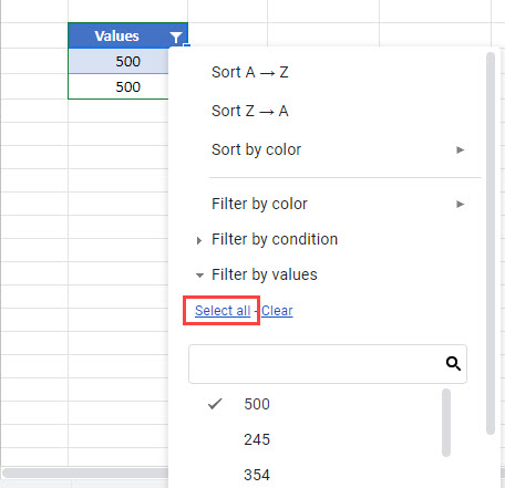
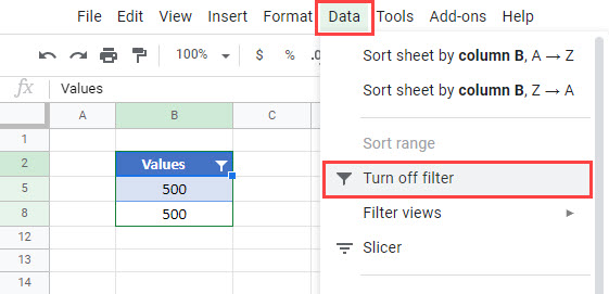
To remove the filter entire, in the Menu, select Data > Turn off Filter.
Find Number in Workbook or Worksheet using FIND in Google Sheets
We can look for values in Google Sheets using the FIND functionality.
- In your workbook, press Ctrl+F on the keyboard.
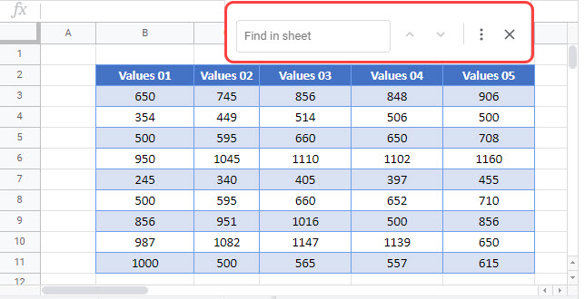
- Type in the value you wish to find.
- All the matching values in the current sheet will be highlighted, with the first one being selected as shown below.
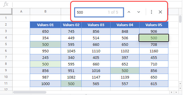
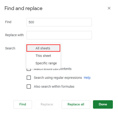
- Select More Options.

- Amend the search to All Sheets.
- Click Find.
- The first instance of the value will be found. Click Find again to go to the next value and continue to click Find to find all the matching values in the workbook.
- Click Done to exit out of the Find and Replace Dialog Box.
Splitting single-cell values into multiple cells, and collating multiple cell values into one, is the part of data manipulation. With the help of the text function in excelTEXT function in excel is a string function used to change a given input to the text provided in a specified number format. It is used when we large data sets from multiple users and the formats are different.read more “LEFT,” “MID,” and “RIGHT,” we can extract part of the selected text value or string value. To make the formula dynamic, we can use other supporting functions like “FIND” and “LEN.” However, the extraction of only numbers with the combination of alpha-numeric values requires an advanced level of formula knowledge.
Table of contents
- How to Extract Number from String in Excel?
- #1 – Extract Number from the String at the End in Excel?
- #2 – Extract Numbers From Right Side but Without Special Characters
- #3 – Extract Number From Any Position in Excel
- Recommended Articles
This article will show you the three ways to extract numbers from a string in Excel.
- #1 – Extract Number from the String at the End of the String
- #2 – Extract Numbers from Right Side but Without Special Characters
- #3 – Extract Numbers from any Position of the String
Below we have explained the different ways of extracting the numbers from strings in Excel. Read the whole article to learn this technique.
You are free to use this image on your website, templates, etc, Please provide us with an attribution linkArticle Link to be Hyperlinked
For eg:
Source: Extract Number from String Excel (wallstreetmojo.com)
#1 – Extract the Number from the String at the End in Excel?
You can download this Extract Number from String Excel Template here – Extract Number from String Excel Template
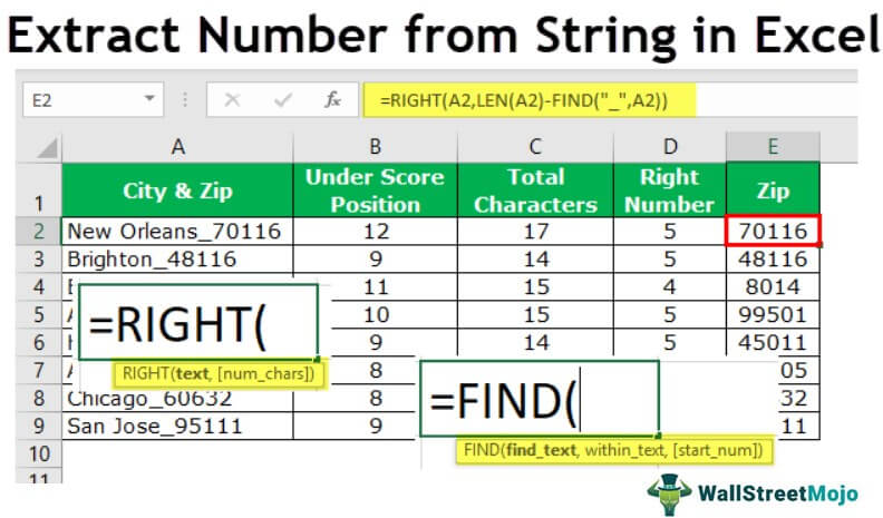
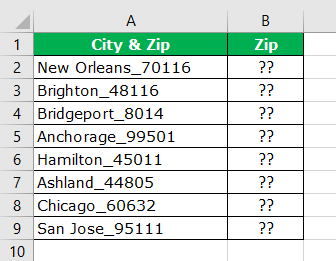
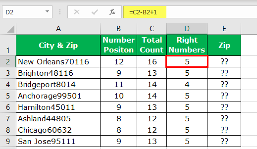
When we get the data, it follows a certain pattern, and having all the numbers at the end of the string is one of the patterns.
- For example, the city with its zip code below is a sample of the same.

- We have the city name and zip code in the above example. In this case, we know we have to extract the zip code from the right-hand side of the string. But, we do not know exactly how many digits we need from the right-hand side of the string.
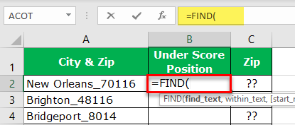
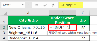
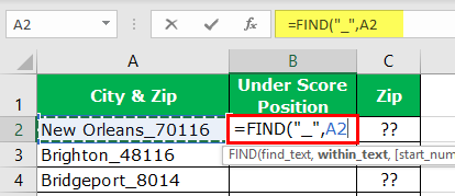
Before the numerical value starts, one of the common things is the underscore (_) character. So first, we need to identify the position of the underscore character. We can do it by using the FIND method. So, apply the FIND function in excel.

- What text do we need to find in the find_text argument? In this example, we need to find the position of the underscore, so enter the underscore in double quotes.

- The within_text is in which text we need to find the mentioned text, so select cell reference.

- The last argument is not required, so leave it as of now.

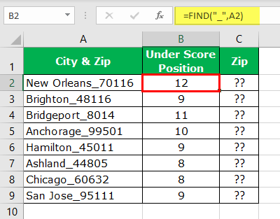
- So, we have got positions of underscore character for each cell. Next, we need to identify how many characters we have in the entire text. So, we must apply the LEN function in Excel to get the total length of the text value.

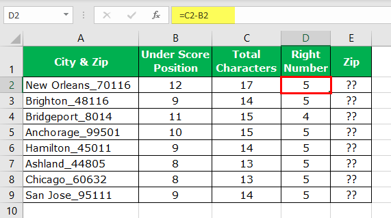
- Now, we have total characters and positions of underscore before the numerical value. Therefore, to supply the number of characters needed for the RIGHT function, we must minus the Total Characters with Underscore Position.

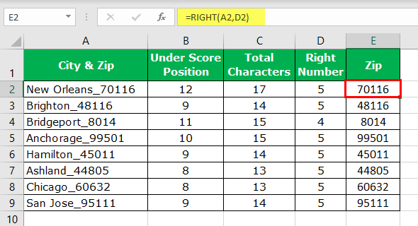
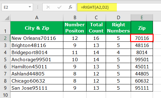
- Now, apply the RIGHT function in cell E2.

- So, like this, we can get the numbers from the right-hand side when we have a common letter before the number starts in the string value. Instead of having so many helper columns, we can apply the formula in a single cell.


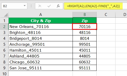
=RIGHT(A2,LEN(A2)-FIND(“_”,A2))
It will eliminate all the supporting columns and reduce the time drastically.
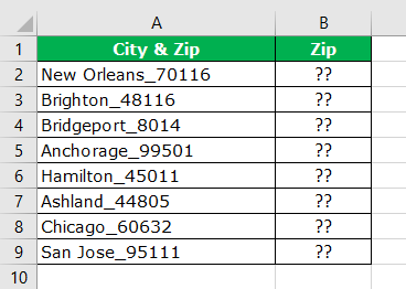
#2 – Extract Numbers From Right Side but Without Special Characters
Assume we have the same data, but this time we do not have any special character before the numerical value.
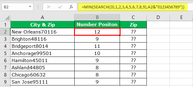
We have found a special character position in the previous example, but we do not have that luxury here. So, the formula below will find the “Numerical Position.”
Please do not turn off your computer by looking at the formula. We will decode this for you.
For the SEARCH function in excelSearch function gives the position of a substring in a given string when we give a parameter of the position to search from. As a result, this formula requires three arguments. The first is the substring, the second is the string itself, and the last is the position to start the search.read more, we have supplied all the possible starting numbers of numbers, so the formula looks for the position of the numerical value. Since we have provided all the possible numbers to the array, the resulting arrays should contain the same numbers. Then, the MIN function in excelIn Excel, the MIN function is categorized as a statistical function. It finds and returns the minimum value from a given set of data/array.read more returns the smallest number among the two, so the formula reads below.
=MIN(SEARCH({0,1,2,3,4,5,6,7,8,9},A2&”0123456789″))
So, now we have the “Numerical Position.” But, first, let us find the total number of characters in the cell.
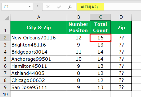
Consequently, it will return the total number of characters in the supplied cell value. Now, the “LEN” – position of the numerical value will return the number of characters required from the right side, so apply the formula to get the number of characters.
Now, we must apply the RIGHT function in excelRight function is a text function which gives the number of characters from the end from the string which is from right to left. For example, if we use this function as =RIGHT ( “ANAND”,2) this will give us ND as the result.read more to get only the numerical part from the string.
Let us combine the formula in a single cell to avoid multiple helper columns.
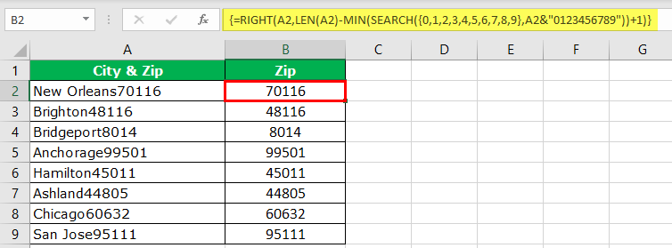
{=RIGHT(A2,LEN(A2)-MIN(SEARCH({0,1,2,3,4,5,6,7,8,9},A2&”0123456789″))+1)}
#3 – Extract Number From Any Position in Excel
We have seen from the RIGHT side extraction. But this is not the case with all the scenarios, so now we will see how to extract numbers from any string position in Excel.
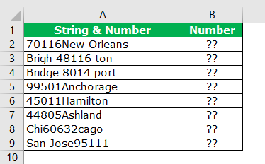
For this, we need to employ various functions of Excel. Below is the formula to extract the numbers from any string position.
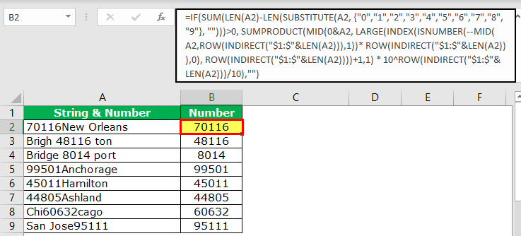
=IF(SUM(LEN(A2)-LEN(SUBSTITUTE(A2, {“0″,”1″,”2″,”3″,”4″,”5″,”6″,”7″,”8″,”9”}, “”)))>0, SUMPRODUCT(MID(0&A2, LARGE(INDEX(ISNUMBER(–MID(A2,ROW(INDIRECT(“$1:$”&LEN(A2))),1))* ROW(INDIRECT(“$1:$”&LEN(A2))),0), ROW(INDIRECT(“$1:$”&LEN(A2))))+1,1) * 10^ROW(INDIRECT(“$1:$”&LEN(A2)))/10),””)
Recommended Articles
This article is a guide to Extract Number From String in Excel. We discussed the top 3 easy methods, step-by-step examples, and a downloadable Excel template. You may learn more about Excel from the following articles: –
- MID Function in Excel
- REPLACE Function in Excel
- Substring in Excel
- VBA String Functions
Extracting numbers from a list of cells with mixed text is a common data cleaning task.
Unfortunately, there is no direct menu or function created in Excel to help us accomplish this.
In this tutorial we will look at three cases where you might have a list of mixed text, from which you might want to extract numbers:
- When the number is always at the end of the text
- When the number is always at the beginning of the text
- When the number can be anywhere in the text
We will look at three different formulas that can be used to extract the numbers in each case.
At the end of the tutorial, we will also take a look at some VBA code that you can use to accomplish the same.
Brace yourself, this might get a little complex!
Extracting a Number from Mixed Text when Number is Always at the End of the Text
Consider the following example:

Here, each cell has a mix of text and numbers, with the number always appearing at the end of the text. In such cases, we will need to use a combination of nested Excel functions to extract the numbers.
The functions we will use are:
- FIND – This function searches for a character or string in another string and returns its position.
- MIN – This function returns the smallest value in a list.
- LEFT – This function extracts a given number of characters from the left side of a string.
- SUBSTITUTE – This function replaces a particular substring of a given text with another substring.
- IFERROR – This function returns an alternative result or formula if it finds an error in a given formula.
Essentially, we will be using the above functions altogether to perform the following sequence of tasks:
- Find the position of the first numeric value in the given cell
- Extract and remove the text part of the given cell (by removing everything to the left of the first numeric digit)
The formula that we will use to extract the numbers from cell A2 is as follows:
=SUBSTITUTE(A2,LEFT(A2,MIN(IFERROR(FIND({0,1,2,3,4,5,6,7,8,9},A2),""))-1),"")
Let us break down this formula to understand it better. We will go from the inner functions to the outer functions:
- FIND({0,1,2,3,4,5,6,7,8,9},A2)
This function tries to find the positions of all the numbers (0-9) in the cell A2. Thus it returns an arrayformula:
{#VALUE!,#VALUE!,#VALUE!,#VALUE!,#VALUE!,#VALUE!,9,7,8,#VALUE!}
It returns a #VALUE! error for all digits except the 7th, 8th, and 9th digits because it was not able to find these numbers (0,1,2,3,4,5,9) in cell A2. It simply returns the positions of numbers 6,7 and 8 which are the 9th, 7th, and 8th characters respectively in A2.
- IFERROR(FIND({0,1,2,3,4,5,6,7,8,9},A2),””)
Next, the IFERROR function replaces all the error elements of the array with a blank (“”). As such it returns the arrayformula:
{“”,””,””,””,””,””,9,7,8,””}
- MIN(IFERROR(FIND({0,1,2,3,4,5,6,7,8,9},A2),””))
After this the MIN function finds the array element with least value. This is basically the position of the first numeric character in A2. The function now returns the value 7.
- LEFT(A2,MIN(IFERROR(FIND({0,1,2,3,4,5,6,7,8,9},A2),””))-1)
At this point we want to extract all text characters from A2 (so that we can remove them). So we want the LEFT function to extract all the characters starting backwards from the 7-1= 6th character. Thus we use the above formula. The result we get at this point is “arnold”. Notice we subtracted 1 from the second parameter of the LEFT function.
- SUBSTITUTE(A2,LEFT(A2,MIN(IFERROR(FIND({0,1,2,3,4,5,6,7,8,9},A2),””))-1),””)
Now all that’s left to do is remove the string obtained, by replacing it with a blank. This can be easily achieved by using the SUBSTITUTE function: We finally get the numeric characters in the mixed text, which is “786”.
Once you are done entering the formula, make sure you press CTRL+SHIFT+Enter, instead of just the return key. This is because the formula involves arrays.
In a nutshell, here’s what’s happening when you break down the formula:
=SUBSTITUTE(A2,LEFT(A2,MIN(IFERROR(FIND({0,1,2,3,4,5,6,7,8,9},A2),””))-1),””)
=SUBSTITUTE(A2,LEFT(A2,MIN(IFERROR({{#VALUE!,#VALUE!,#VALUE!,#VALUE!,#VALUE!,#VALUE!,9,7,8,#VALUE!}),””))-1),””)
=SUBSTITUTE(A2,LEFT(A2,MIN({“”,””,””,””,””,””,9,7,8,””}))-1),””)
=SUBSTITUTE(A2,”arnold”,””)
=786
When you drag the formula down to the rest of the cells, here’s the result you get:

Also read: How to Generate Random Letters in Excel?
Extracting a Number from Mixed Text when Number is Always at the Beginning of the Text
Now let us consider the case where the numbers are always at the beginning of the Text.
Consider the following example:

Here, each cell has a mix of text and numbers, with the number always appearing at the beginning of the text. In such cases, we will again need to use a combination of nested Excel functions to extract the numbers.
In addition to the functions we used in the previous formula, we are going to use two additional functions. These are:
- MAX – This function returns the largest value in a list
- RIGHT – This function extracts a given number of characters from the right side of a string
- LEN – This function finds the length of (number of characters in) a given string.
Essentially, we will be using these functions altogether to perform the following sequence of tasks:
- Find the position of the last numeric value in the given cell
- Extract and remove the text part of the given cell (by removing everything to the right of the last numeric digit)
The formula that we will use to extract the numbers from cell A2 is as follows:
=SUBSTITUTE(A2,RIGHT(A2,LEN(A2)-MAX(IFERROR(FIND({0,1,2,3,4,5,6,7,8,9},A2),""))),"")
Let us break down this formula to understand it better. We will go from the inner functions to the outer functions:
- FIND({0,1,2,3,4,5,6,7,8,9},A2)
This function tries to find the positions of all the numbers (0-9) in the cell A2. Thus it returns an arrayformula:
{#VALUE!,#VALUE!,1,#VALUE!,#VALUE!,2,#VALUE!,#VALUE!,#VALUE!,#VALUE!}
It returns a #VALUE! error for all digits except the 3rd and 6th digits because it was not able to find these numbers (0,1,3,4,6,7,8,9) in cell A2. It simply returns the positions of numbers 2 and 5 which are the 1st and 2nd characters respectively in A2.
- IFERROR(FIND({0,1,2,3,4,5,6,7,8,9},A2),””)
Next, the IFERROR function replaces all the error elements of the array with a blank. As such it returns the array formula:
{“”,””,1,””,””,2,””,””,””,””}
- MAX(IFERROR(FIND({0,1,2,3,4,5,6,7,8,9},A2),””))
After this the MAX function finds the array element with the highest value. This is basically the position of the last numeric character in A2. The function now returns the value 2.
- LEN(A2)-MAX(IFERROR(FIND({0,1,2,3,4,5,6,7,8,9},A2),””))
At this point we want to extract all text characters from A2 (so that we can remove them). We need to specify how many characters we want to remove. This is obtained by computing the length of the string in A2 minus the position of the last numeric value.Thus we will get the value 8-2 = “6”.
- RIGHT(A2,LEN(A2)-MAX(IFERROR(FIND({0,1,2,3,4,5,6,7,8,9},A2),””)))
We can now use the RIGHT function to extract 6 characters starting from the 2nd character onwards. The result we get at this point is “arnold”.
- SUBSTITUTE(A2,RIGHT(A2,LEN(A2)-MAX(IFERROR(FIND({0,1,2,3,4,5,6,7,8,9},A2),””))),””)
Now all that’s left to do is remove this string by replacing it with a blank. This is easily achieved by using the SUBSTITUTE function. We finally get the numeric characters in the mixed text, which is “25”.
Again, once you are done entering the formula, don’t forget to press CTRL+SHIFT+Enter, instead of just the return key.
In a nutshell, here’s what’s happening when you break down the formula:
=SUBSTITUTE(A7,RIGHT(A7,LEN(A7)-MAX(IFERROR(FIND({0,1,2,3,4,5,6,7,8,9},A7),””))),””)
=SUBSTITUTE(A7,RIGHT(A7,LEN(A7)-MAX(IFERROR({#VALUE!,#VALUE!,1,#VALUE!,#VALUE!,2,#VALUE!,#VALUE!,#VALUE!,#VALUE!}
),””))),””)
=SUBSTITUTE(A7,RIGHT(A7,LEN(A7)-MAX({“”,””,1,””,””,2,””,””,””,””}
)),””)
=SUBSTITUTE(A7,RIGHT(A7,LEN(A7)-2),””)
=SUBSTITUTE(A7,RIGHT(A7,8-2),””)
=SUBSTITUTE(A7,”arnold”,””)
=25
When you drag the formula down to the rest of the cells, here’s the result you get:

Extracting a Number from Mixed Text when Number can be Anywhere in the Text
Finally let us consider the case where the numbers can be anywhere in the text, be it the beginning, end or middle part of the text.
Let’s take a look at the following example:

Here, each cell has a mix of text and numbers, where the number appears in any part of the text. In such cases, we will need to use a combination of nested Excel functions to extract the numbers.
Here are the functions that we are going to use this time:
- INDIRECT – This function simply returns a reference to a range of values.
- ROW – This function returns a row number of a reference.
- MID – This function extracts a given number of characters from the middle of a string.
- TEXTJOIN – This function combines text from multiple ranges or strings using a specified delimiter between them.
Note that the formula discussed in this section will work only in Excel version 2016 onwards as it uses the newly introduced TEXTJOIN function. If you are using an older version of Excel, then you may consider using the VBA method instead (discussed in the next section).
In this method, we will essentially be using the above functions altogether to perform the following sequence of tasks:
- Break up the given text into an array of individual characters
- Find out and remove all characters that are not numbers
- Combine the remaining characters into a full number
The formula that we will use to extract the numbers from cell A2 is as follows:
=TEXTJOIN("",TRUE,IFERROR(MID(A2,ROW(INDIRECT("1:"&LEN(A2))),1)*1,""))
Let us break down this formula to understand it better. We will go from the inner functions to the outer functions:
- LEN(A2)
This function finds the length of the string in cell A2. In our case it returns 13.
- INDIRECT(“1:”&LEN(A2))
This function just returns a reference to all the rows from row 1 to row 12.
- ROW(INDIRECT(“1:”&LEN(A2)))
Now this function returns the row numbers of each of these rows. In other words, it simply returns an array of numbers 1 to 12. This function thus returns the array:
{1;2;3;4;5;6;7;8;9;10;11;12;13}
Note: We use the ROW() function instead of simply hard-coding an array of numbers 1 to 12 because we want to be able to customize this formula depending on the size of the string being worked on. This will ensure that the function adjusts itself when copied to another cell. ·
- MID(A2,ROW(INDIRECT(“1:”&LEN(A2))),1)
Next the MID function extracts the character from A2 that corresponds to each position specified in the array. In other words, it returns an array containing each character of the text in A2 as a separate element, as follows:
{“a”;”r”;”n”;”o”;”l”;”d”;”1″;”4″;”3″;”b”;”l”;”u”;”e”}
- IFERROR(MID(A2,ROW(INDIRECT(“1:”&LEN(A2))),1)*1,””)
After this, the IFERROR function replaces all the elements of the array that are non-numeric. This is because it checks if the array element can be multiplied by 1. If the element is a number, it can easily be multiplied to return the same number. But if the element is a non-numeric character, then it cannot be multiplied with 1 and thus returns an error.
The IFERROR function here specifies that if an element gives an error on multiplication, the result returned will be blank. As such it returns the arrayformula:
{“”;””;””;””;””;””;1;4;3;””;””;””;””}
- TEXTJOIN(“”,TRUE,IFERROR(MID(A2,ROW(INDIRECT(“1:”&LEN(A2))),1)*1,””))
Finally, we can simply combine the array elements together using the TEXTJOIN function. The TEXTJOIN function here combines the string characters that remain (which are the numbers only) and ignores the empty string characters. We finally get the numeric characters in the mixed text, which is “143”.
Once you are done entering the formula, don’t forget to press CTRL+SHIFT+Enter, instead of just the return key.
In a nutshell, here’s what’s happening when you break down the formula:
=TEXTJOIN(“”,TRUE,IFERROR(MID(A2,ROW(INDIRECT(“1:”&LEN(A2))),1)*1,””))
=TEXTJOIN(“”,TRUE,IFERROR(MID(A2,ROW(INDIRECT(“1:”&13)),1)*1,””))
=TEXTJOIN(“”,TRUE,IFERROR(MID(A2,{1;2;3;4;5;6;7;8;9;10;11;12;13},1)*1,””))
=TEXTJOIN(“”,TRUE,IFERROR({“a”;”r”;”n”;”o”;”l”;”d”;”1″;”4″;”3″;”b”;”l”;”u”;”e”}
*1,””))
=TEXTJOIN(“”,TRUE,IFERROR(MID(A2,{1;2;3;4;5;6;7;8;9;10;11;12;13},1)*1,””))
=TEXTJOIN(“”,TRUE, {“”;””;””;””;””;””;1;4;3;””;””;””;””})
=143
When you drag the formula down to the rest of the cells, here’s the result you get:

Using VBA to Extract Number from Mixed Text in Excel
The above method works well enough in extracting numbers from anywhere in a mixed text.
However, it requires one to use the TEXTJOIN function, which is not available in older Excel versions (versions before Excel 2016).
If you’re on a version of Excel that does not support TEXTJOIN, then you can, instead, use a snippet of VBA code to get the job done.
If you have never used VBA before, don’t worry. All you need to do is copy the code below into your VBA developer window and run it on your worksheet data.
Here’s the code that you will need to copy:
'Code by Steve Scott from spreadsheetplanet.com
Function ExtractNumbers(CellRef As String)
Dim StringLength As Integer
StringLength = Len(CellRef)
For i = 1 To StringLength
   If (IsNumeric(Mid(CellRef, i, 1))) Then Result = Result & Mid(CellRef, i, 1)
Next i
ExtractNumbers = Result
End Function
The above code creates a user-defined function called ExtractNumbers() that you can use in your worksheet to extract numbers from mixed text in any cell.
To get to your VBA developer window, follow these steps:
- From the Developer tab, select Visual Basic.

- Once your VBA window opens, Click Insert->Module. That’s it, you can now start coding.

Type or copy-paste the above lines of code into the module window. Your code is now ready to run.

Now, whenever you want to extract numbers from a cell, simply type the name of the function, passing the cell reference as a parameter. So to extract numbers from a cell A2, you will simply need to type the function as follows in a cell:
=ExtractNumbers(A2)

Explanation of the Code
Now let us take some time to understand how this code works.
- In this code, we defined a function named ExtractNumbers, that takes the string in the cell we want to work on. We assigned the name CellRef to this string.
Function ExtractNumbers(CellRef As String)
- We created a variable named StringLength, that will hold the length of the string, CellRef.
Dim StringLength As Integer
StringLength = Len(CellRef)
- Next, we loop through each character in the string CellRef and find out if it is a number. We use the function Mid(CellRef, i, 1) to extract a character from the string at each iteration of the loop. We also use the IsNumeric() function to find out if the extracted character is a number. Each extracted numeric character is combined together into a string called Result.
For i = 1 To StringLength
If (IsNumeric(Mid(CellRef, i, 1))) Then Result = Result & Mid(CellRef, i, 1)
Next i
- This Result is then returned by the function.
ExtractNumbers = Result
Note that since the workbook now has VBA code in it, you need to save it with .xls or .xlsm extension.
You can also choose to save this to your Personal Macro Workbook, if you think you will be needing to run this code a lot. This will allow you to run the code on any Excel workbook of yours.
Well, that was a lot!
In this tutorial, we showed you how to extract numbers from mixed text in excel.
We saw three cases where the numbers are situated in different parts of the text. We also showed you how to use VBA to get the task done quickly.
Other Excel articles you may also like:
- How to Extract URL from Hyperlinks in Excel (Using VBA Formula)
- How to Reverse a Text String in Excel (Using Formula & VBA)
- How to Add Text to the Beginning or End of all Cells in Excel
- How to Remove Text after a Specific Character in Excel (3 Easy Methods)
- How to Separate Address in Excel?
- How to Extract Text After Space Character in Excel?
- How to Find the Last Space in Text String in Excel?
- How to Remove Space before Text in Excel

The Find and Replace tool is a powerful yet often forgotten feature of Excel. Let’s see how it can be used to find and replace text and numbers in a spreadsheet and also some of its advanced features.
When working with large spreadsheets, it is a common task to need to find a specific value. Fortunately, Find and Replace make this a simple task.
Select the column or range of cells you want to analyze or click any cell to search the entire worksheet. Click Home > Find & Select > Find or press the Ctrl+F keyboard shortcut.

Type the text or number you want to search for in the “Find What” text box.
Click “Find Next” to locate the first occurrence of the value in the search area; click “Find Next” again to find the second occurrence, and so on.
Next, select “Find All” to list all occurrences of the value including information, such as the book, sheet, and cell where it is located. Click on the item in the list to be taken to that cell.
Finding specific or all occurrences of a value in a spreadsheet is useful and can save hours of scrolling through.
If you want to change the occurrences of a value with something else, click the “Replace” tab. Type the text or number you want to use as a replacement value within the “Replace With” text box.
Click “Replace” to change each occurrence one at a time or click “Replace All” to change all occurrences of that value in the selected range.
RELATED: How to Add Text to a Cell With a Formula in Excel
Explore the Advanced Options
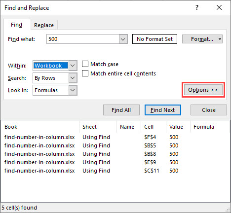
Find and Replace has advanced features that many users are not aware of. Click the “Options” button to expand the window and see these.
One really useful setting is the ability to change from looking within the active worksheet to the workbook.
Click the “Within” list arrow to change this to Workbook.
Other useful options include the “Match Case” and “Match Entire Cell Contents” checkboxes.
These options can help narrow down your search criteria, ensuring you find and replace the correct occurrences of the values you’re looking for.
Change the Formatting of Values
You can also find and replace the formatting of values.
Select the range of cells you want to find and replace in or click any cell to search the entire active worksheet.
Click Home > Find & Select > Replace to open the Find and Replace dialog box.
Select the “Options” button to expand the Find and Replace options.
You do not need to enter text or numbers that you want to find and replace unless required.
Click the “Format” button next to the “Find What” and “Replace With” text boxes to set the formatting.
Specify the formatting you want to find or replace.
A preview of the formatting is shown in the Find and Replace window.
Continue with any other options you want to set and then click “Replace All” to change all occurrences of the formatting.
Using Wildcard Characters
When using Find and Replace, sometimes you might need to perform partial matches using wildcard characters.
There are two wildcard characters you can use in Find and Replace. The question mark and the asterisk. The question mark (?) is used to find a single character. For example, Al?n would find “Alan,” “Alen,” and “Alun.”
The asterisk (*) replaces any number of characters. For example, y* would find “yes,” “yeah,” “yesss,” and “yay.”
In this example, we have a list of names followed by an ID in column A of our spreadsheet. They follow this format: Alan Murray – 5367.
We want to replace all occurrences of the ID with nothing to remove them. This will leave us with just the names.
Click Home > Find & Select > Replace to open the Find and Replace dialog box.
Type ” – *” in the “Find What” text box (there are spaces before and after the hyphen). Leave the “Replace With” text box empty.
Click “Replace All” to modify your spreadsheet.
READ NEXT
- › How to Find the Smallest or Largest Number in Microsoft Excel
- › How to Use the SUBSTITUTE Function in Microsoft Excel
- › How to Remove Duplicate Rows in Excel
- › 9 Useful Microsoft Excel Functions for Working With Text
- › How to Remove Spaces in Microsoft Excel
- › 5 Ways to Convert Text to Numbers in Microsoft Excel
- › How to Use the Navigation Pane in Microsoft Excel
- › The New NVIDIA GeForce RTX 4070 Is Like an RTX 3080 for $599