
To start a new line of text or add spacing between lines or paragraphs of text in a worksheet cell, press Alt+Enter to insert a line break.
-
Double-click the cell in which you want to insert a line break.
-
Click the location inside the selected cell where you want to break the line.
-
Press Alt+Enter to insert the line break.
To start a new line of text or add spacing between lines or paragraphs of text in a worksheet cell, press CONTROL + OPTION + RETURN to insert a line break.
-
Double-click the cell in which you want to insert a line break.
-
Click the location inside the selected cell where you want to break the line.
-
Press CONTROL+OPTION+RETURN to insert the line break.
To start a new line of text or add spacing between lines or paragraphs of text in a worksheet cell, press Alt+Enter to insert a line break.
-
Double-click the cell in which you want to insert a line break (or select the cell and then press F2).
-
Click the location inside the selected cell where you want to break the line.
-
Press Alt+Enter to insert the line break.
-
Double-tap within the cell.
-
Tap the place where you want a line break, and then tap the blue cursor.

-
Tap New Line in the contextual menu.

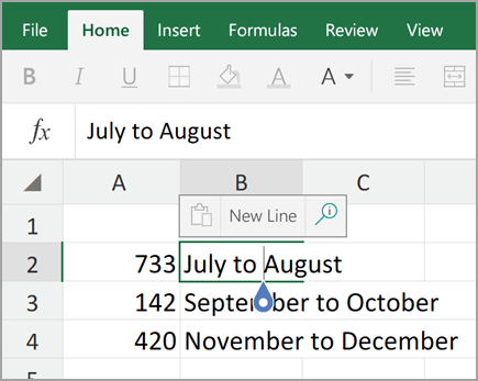
Note: You cannot start a new line of text in Excel for iPhone.
-
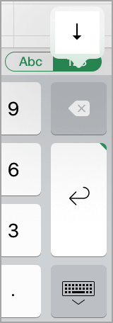
Tap the keyboard toggle button to open the numeric keyboard.
-
Press and hold the return key to view the line break key, and then drag your finger to that key.

Lines in Excel are used to show connections between two or more data points. However, we can also draw lines without showing any types of relationships in Excel. To draw a line in Excel, we need to go to the “Insert” tab and click on “Shapes,” then, we can choose the type of line we want to draw in Excel.
Table of contents
- Draw and Insert a Line in Excel
- How to Insert/Draw a Line in Excel?
- How to Draw a Line in Excel?
- Insert Line in Excel Example #1
- Insert Line in Excel Example #2
- Explanation of Draw Lines in Excel
- Things to Remember
- Recommended Articles
Earlier, if we needed to draw a particular shape in a document, it was done by a drawing program. The program was separate from the software itself. In this way, the software was dependent on the drawing program if there needed to be any connections drawn out.
But now, in Microsoft Excel, it is easier to draw shapes of any size or desire. So, for example, we can draw a circle, a line, a rectangle, or any shape.
How to Insert/Draw a Line in Excel?
Excel has provided us with the tools required to insert a line or shape or draw a shape in it, rather than depending upon any other third program. In addition, it has a variety of shapes that we can use as the situation requires.
One of the shapes is a “Line.” The line is a collection of points that extends in both directions. We can use it to form certain shapes, such as squares or rectangles, or it can just be a straight line that has an infinite ending to both ends.
The main question arises: how do we draw a line in Excel?
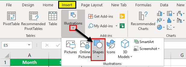
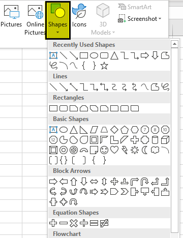
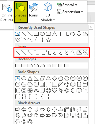
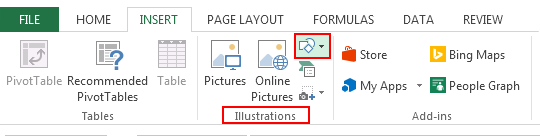
If we go to the “Insert” tab and in the “Illustrations” section, we will find an option for “Shapes.”
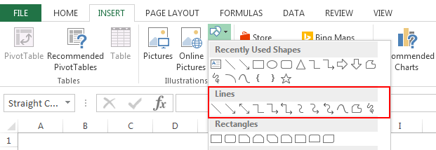
If we click on “Shapes,” it gives us a variety of shapes to choose from. One of the varieties is the “Lines.”
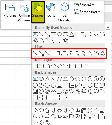
Now, in the line option, we have various types of line options to choose from:
- Line
- Arrow
- Double Arrow
- Elbow Connector
- Elbow Arrow Connector
- Elbow Double Arrow Connector
- Curved Connector
- Curved Arrow Connector
- Curved Double Arrow Connector
- Curve
- FreeForm
- Scribble.
All of these forms of lines are used as a connector in Excel. It shows the relationship, dependency, or connection in Excel. For example, suppose we have various cells with data but which cells refer to which data can be recognized by inserting a line or shape in Excel.
How to Draw a Line in Excel?
To draw a line in Excel, we must follow these steps:
- In the “Insert” tab under “Illustrations,” click on “Shapes.”
- When the dialog box appears, we must go to the “Lines” section,
- Select any line from the various given options to draw a connection.
Like this, we use the elbow arrow connector in “Lines.”
Let us learn how to draw a line in Excel by a few examples:
You can download this Draw Line Excel Template here – Draw Line Excel Template
Insert Line in Excel Example #1
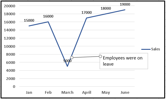
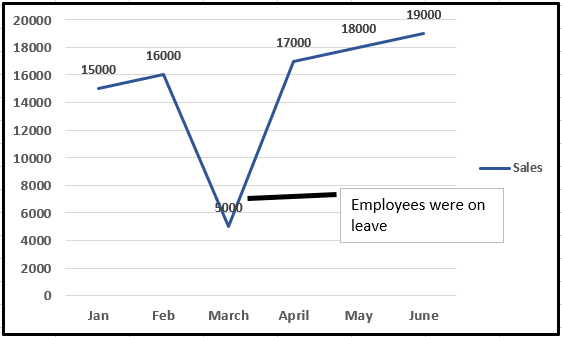
Suppose we have a chart for data. We can see that there is a dip in sales for a company. Rather than going through the whole data and analyzing the issue for a viewer, the chart author can add text to show the reason for the spike and draw a line in Excel to indicate the same.
Have a look at the chart below.
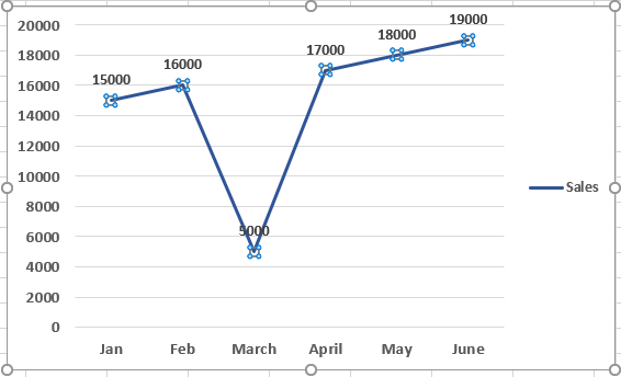
Looking at the chart, we see that they dipped in sales in March, but we do not know why.
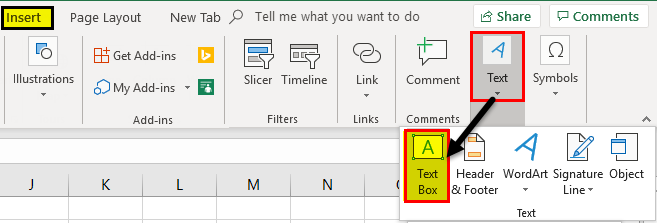
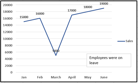
- We must first insert a text box and write the text for the dip in sales. Then, we must insert a line to indicate the reason.

- Write the text in the text box.

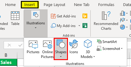
- Now, in the Insert tab under llustrations, click on Shapes.

- A dialog box pops up for different shapes. Select the Lines menu.

- In the Lines option, we can see the option for line shape, which is the first one.

- Now, we must right-click on the mouse and start stretching the line to the extent we want it and release the mouse.

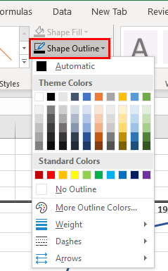
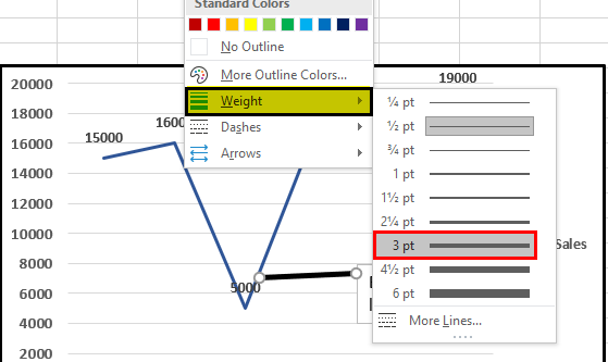
- Next, in the Shape Outline option, click on Weight.

- A dialog box pops up with the various weights or the dimensions for the line. Select anyone suitable like 3 points.

- We have successfully drawn a line for the chart to indicate a connection.


Insert Line in Excel Example #2
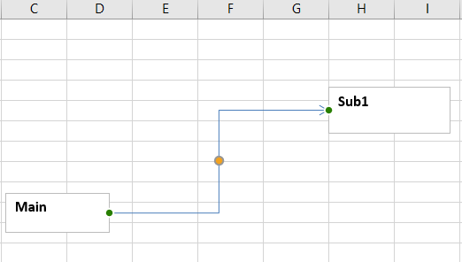
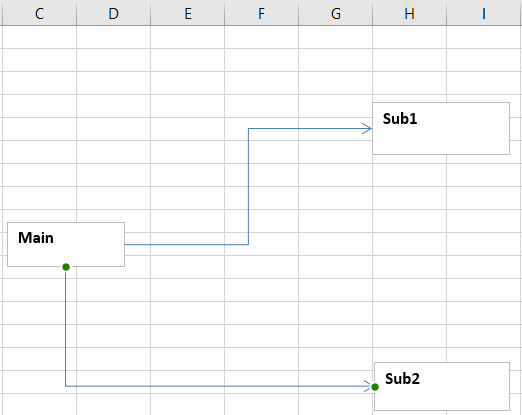
Suppose we have an illustration such as below somewhere in our data. We want to show a relationship between them.
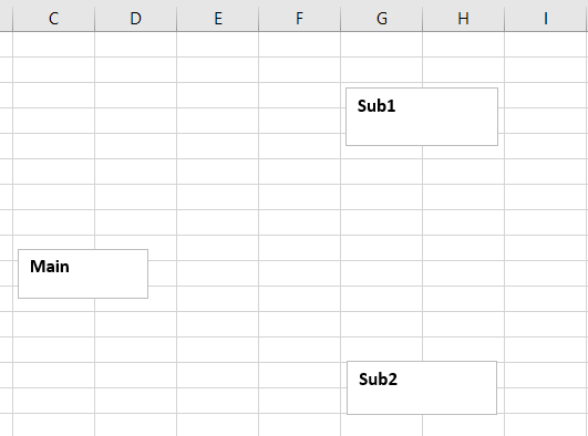
We will use the elbow arrow connector in line to show that the main is related to both sub 1 and sub2.
Step #1 – In the “Illustrations” under the “Insert” tab, click on “Shapes.”

Step #2 – Again, a dialog box may appear for the various shapes.
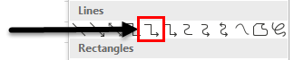
Step #3 – This time, we will choose the “Elbow Arrow” connector, located in the fifth position from the start.
Step #4 – Now we know we need to show a relation between the main and the two subs. Right-click on the mouse from the main and release the mouse when we drag it to the sub 1 end.
Step #5 – This is the first connection. Now again, go to the “Insert” tab and, in “Illustrations,” click on “Shapes.”
Step #6 – Then, click on the “Elbow Arrow” connector in “Lines.”

Step #7 – Again, start from the main by right click and release the click in the sub 2’s end.
Explanation of Draw Lines in Excel
The lines in Excel are inserted to show connections between two points.
We can also use it to draw shapes if used in free form. For example, “Draw the line” in Excel acts as a connector as in the above example. It showed the connection between the main and the other two subs.
Things to Remember
- Lines should start at one point and end at another point.
- To start inserting a line in Excel, we must right-click on the mouse, stretch the line, and release the click when we want to end the line.
Recommended Articles
This article is a guide to Draw Line in Excel. We discuss how to insert/draw a Line in Excel, practical examples, and a downloadable Excel template. You may learn more about Excel from the following articles: –
- Border in Excel
- How to Make a Chart in Excel?
- Use Format Painter in Excel
- Insert Worksheet in Excel
- Forecast in Excel
Excel is not only a wonderful tool for data entry and data analysis, but also great at making charts, flow charts, simple diagrams, etc.
It’s quite simple in Excel to insert a line and then customize and position it. In fact, you’ll be surprised how many options you get when you need to draw a line in Excel.
You can easily draw a line to connect two boxes (to show the flow) or add a line in an Excel chart to highlight some specific data point or the trend.
Excel also allows you to use your cursor or touch screen option to manually draw a line or create other shapes.
How to Insert a Line in Excel (Using Illustation)
To insert a line in the worksheet in Excel, you need to use the Shapes option. It inserts a line as a shape object that you can drag and place anywhere in the worksheet.
You can also easily customize it- such as change the size, thickness, color, add effects such as shadow, etc.
Below are the steps to insert a line shape in Excel:
- Open the Excel workbook and activate the worksheet in which you want to draw/insert the line
- Click the Insert tab

- Click on Illustrations
- Click on the Shapes icon

- Choose from any of the existing 12 Line options
- Go to the worksheet, click the left key on your mouse/trackpad and drag the cursor to insert a line of that length

The above steps would instantly insert the line that you selected in step 5.
These are the 12 line options that you have available in Excel:
- Straight Line
- Line Arrow (with arrow at one end of the line)
- Line Arrow Double (arrow at both ends)
- Connector: Elbow (use this to connect boxes, this is not a straight line)
- Connector: Elbow arrow (arrow at one end)
- Connector: Elbow double-arrow (arrow at both ends)
- Connector: Curved
- Connector: Curved Arrow
- Connector: Curved Double-Arrow
- Curve
- Freeform: Shape
- Freeform: Scribble
Adding Multiple Lines in One Go
When you use the above steps, you can only insert any of the line shapes once. If you need to insert it again (say you want to insert 3 lines), you will have to repeat the process two times again.
Instead, you can lock the drawing mode so you can keep inserting the lines in one go.
Below are the steps to lock the line drawing mode:
- Open the Excel workbook and activate the worksheet in which you want to draw/insert the line
- Click the Insert tab
- Click on Illustrations
- Click on the Shapes icon
- Right-click on any of the line shapes that you want lock (i.e., the one that you want to insert multiple times)
- Click on Lock Drawing Mode

- Click anywhere in the worksheet
When you do the above steps, you will notice that your cursor changes and remains a plus icon. You can now click and drag and insert multiple lines in one go.
To unlock the line drawing mode, hit the Escape key.
Customizing Lines/Arrows in Excel
Apart from inserting different types of lines, you can also further customize the line shapes you insert.
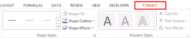
When you click on any of the line shapes in the worksheet, you will see a new contextual tab appear in the ribbon – the Shape Format tab.

In this new tab, you get some additional options to format the lines.
Shape Styles Options
In the Shape Styles group, there are some inbuilt theme styles and preset styles you can use. To see all these options, you can click on the More icon.
Then you can select any of the existing styles and it will be applied to all the selected lines in the worksheet.

Apart from this, you can also change the line outline by clicking on the Shape Outline option.

In Shape Outline, you can change the following:
- Color of the line
- Weight of the line (thickness)
- Style of the line (solid, dot, dash, etc)
- Arrows
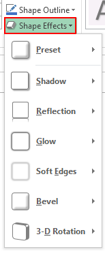
And finally, you can also add some Effects to the line, such as shadow, glow, or reflection. This can be done using the Shape Effect options.

To use these, select one or multiple lines to which you want to add the Effects and then use the options in Shape Effect.
Arranging the Lines
If you’re working with more than a few line shapes in Excel, you will find it useful to know about the ‘Arrange’ options.
You can find these in the Arrange group in the Shape Format tab (which only appears when you select any shape in the worksheet).

Following are the options that are available to you:
- Bring Forward / Send Backward – in case you want to rearrange the shapes
- Selection Pane – this opens a pane on the right where you can see all the shapes in the worksheet. You also have the option to hide some shapes from this pane
- Align – To align the lines left/center/right or top/middle/bottom. This comes in handy when working with multiple shapes where you want these shapes to be neatly aligned
- Rotate – to change the angle to the line
- Group – to group mutiple lines/shapes. For example, you can group lines and boxes using this so they will move/size together.
Note that most of the shape ‘Arrange options’ will become available only when you have more than one shape in the worksheet.
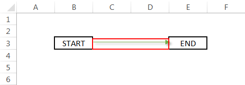
Example 1 – Adding a Line to Connect Boxes/Shapes
Now that I’ve covered the basics of how to insert and format line shapes in Excel, let me show you a couple of examples of how you can use this in real life.
A common example is when you have boxes in the worksheet and you want to connect these boxes using lines. These could be simple lines or lines with arrows that also show the flow
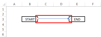
Below I have an example, where I have two boxes, and I want to draw lines between these to connect them.

Below are the steps to do this:
- Click the Insert tab
- Click on Illustrations
- Click on Shapes
- Click on the Line icon
- In the worsheet, click on the right border of the first box and drag the cursor to the left border of the second box.
This will insert a line and you will get something as shown below.
You can also use different styles of the lines, such as with arrows or connectors.
Example 2 – Adding a Line in Excel Charts
Apart from connecting boxes and making flowcharts, arrows are also useful when you want to highlight specific data points in a chart in Excel.
Below is an example where I wanted to highlight one specific data point with some context, so I added some text in the chart and then used an arrow to point that text towards one specific data point.

You can format the line using the same colors used in the chart, or you can use a contrasting color to make it stand out.
How to Draw a Line in Excel (Using Cursor / Touch)
So far, I have covered how to insert a line shape in Excel that you can drag and drop anywhere in the worksheet and format the colors, thickness, etc.
But there is also an option to manually draw a line or shape in Excel.
The Draw option in Excel allows you to use your cursor (or a pen or touch if you have a touch screen) and draw on the screen.
You can use it to quickly draw some shapes and lines – such as a simple flow chart or an organization chart.
It won’t look as neat and clean as the shapes that you can insert, but in some cases, it could be faster and more useful – for example, if you are trying to show a process in excel on a call or in a presentation.
You can access these options in the Draw tab in the ribbon, where you can select the pen (with different colors and thickness) and use it for drawing lines or shapes.

You can change the pen color and size by clicking on the downward arrow that appears when you select any pen.
In case you don’t see the Draw option in the ribbon, right-click on any of the existing ribbon options and click on Customize the Ribbon. In the Excel Options dialog box that opens, check the Draw option (in the right pane) and click OK.
While using the Draw option is quite easy and self-explanatory, there is one useful feature that I want to highlight – Ink to Shape.
Using the Ink to Shape option, you can draw lines and shapes in the worksheet, and then use this option to convert these into neat-looking shapes (such as proper straight lines and boxes/squares/rectangles).
Below is an example of something I drew using my cursor.

And now below are the steps to convert these hand draw boxes and lines into proper shapes:
- Click the Select Object option in the Draw tab
- Select the shapes you want to convert
- Click on the Ink to Shape option
Here is the result I got:

The above option will try its best to convert your free-form hand-drawn shapes into proper lines and boxes.
This feature is not perfect sometimes can’t understand the shapes. But it still works well and can save you a lot of time if you have a lot of these hand-drawn shapes that need to be converted.
In this tutorial, I covered how to draw a line in Excel using the insert shapes options and the draw options.
I hope you found this tutorial useful!
Other Excel tutorials you may also like:
- How to Split a Cell Diagonally in Excel (Insert Diagonal Line)
- How to Remove Dotted Lines in Excel (3 Easy Fix)
- How to Add a TrendLine in Excel Charts
- How to Insert and Use a Radio Button (Option Button) in Excel
![]()
Download Article
![]()
Download Article
Grid lines, which are the faint lines that divide cells on a worksheet, are displayed by default in Microsoft Excel. You can enable or disable them by worksheet, and even choose to see them on printed pages. Gridlines are different than cell borders, which you can add to cells and ranges and customize with line styles and colors. This wikiHow article will show you how to show gridlines in your Excel worksheet, both on the screen and printed, as well as how to add cell borders to make your data stand out.
Things You Should Know
- On Windows, open your Excel sheet. Go to File > Options > Advanced > «Display options for this worksheet». Choose your worksheet and select «Show gridlines.»
- On Mac, open your Excel sheet. Click the Page Layout tab. Find the «Gridlines» panel and check the «View» box.
- Add borders to cells in both OS’s by selecting your cells and clicking Home. Click the arrow next to the Borders icon and choose a style.
-
1
Open the workbook you want to edit. Gridlines always appear on worksheets by default, but you can enable or disable them for any individual worksheet in your settings.
- If the issue is that you can see gridlines on your worksheet but aren’t seeing them on printed pages, you can just enable gridlines when printing. Skip to Step 8 to learn how.
- If you see gridlines on the page but want to add more obvious borders around certain cells or ranges, see Adding Cell Borders in Windows and macOS.
-
2
Click the File menu and select Options. The Excel Options window will expand.
Advertisement
-
3
Click the Advanced tab. It’s in the left panel.
-
4
Scroll down to the «Display options for this worksheet» area. It’s in the right panel just after the «Display options for this workbook» group.
-
5
Select the sheet that doesn’t have gridlines from the «Display options for this worksheet» menu. If you already see the name of the active worksheet here, you can skip this step.
-
6
Check the box next to «Show gridlines.» If gridlines were hidden, the checkbox would be blank. Clicking the box re-enables gridlines.
- If there was already a check next to «Show gridlines» but you don’t see lines on your sheet, the color may be too light. Click the «Gridline color» menu to choose a darker gray color.
-
7
Click OK. Gridlines are now visible on your worksheet.
-
8
Show gridlines when printing (optional). Gridlines, by default, do not appear on printed versions of your worksheet. If you want to see gridlines when you print, you’ll need to enable them in your Page Setup options. Here’s how:
- Click the name of the sheet you want to print at the bottom of your workbook.
- Click the Page Layout tab at the top.
- Click the small arrow at the bottom-right corner of the «Page Setup» panel in the toolbar.
- Click the Sheet tab.
- Check the box next to «Gridlines» under «Print.»
- Click OK. Now when you print this sheet, gridlines will appear on each page.


Advertisement
-
1
Open the workbook you want to edit. Gridlines always appear on worksheets by default, but you can enable or disable them for any individual worksheet in your settings.
- If you already see gridlines on the page but want to add more obvious borders around certain cells or ranges, see Adding Cell Borders in Windows and macOS.
- If your workbook is not open to the sheet that doesn’t have gridlines, click the name of that sheet at the bottom of the workbook to open it now.
-
2
Click the Page Layout tab. It’s at the top of Excel.[1]
-
3
Check the box next to «View» on the «Gridlines» panel. This is in the toolbar at the top of Excel. As long as this box is checked, gridlines will be visible for this worksheet on the screen.
-
4
(optional) Check the box next to «Print» to print gridlines. If you want to see gridlines on the printed version of your worksheet, this option ensures they’ll show up.


Advertisement
-
1
Open your workbook in Excel. Gridlines appear on all sheets by default, but they may not be bold enough to make your data stand out. If you want to surround certain data with more visible lines, you can add borders to those cells.
-
2
Select the range of cells you want to add borders to. You will be able to add a border that surrounds the entire selected range, and/or around each individual cell in the range.[2]
-
3
Click the Home tab. It’s at the top of Excel.
-
4
Click the arrow next to the Borders icon. The Borders icon is a dotted grid on the «Font» panel at the top of Excel. A list of border styles will appear.
-
5
Select a border style. If you want to add darker grid lines that surround each selected cell, choose All Borders. Otherwise, choose any of the other options, such as Outside Borders, which adds one solid border around the selected range.
-
6
Click the arrow next to the «Borders» icon again. Now that you’ve inserted some cell borders, you can customize how they look.
-
7
Click More Borders…. It’s at the bottom of the menu.
-
8
Choose your border options.
- To customize the actual line used in the border (such as changing a solid line to a dotted line), select one of the line styles from the Styles area.
- To make the border a different color, choose a color from the Color menu.
-
9
Click OK. This adds your border preferences to the selected range.
- To remove cell borders, click the arrow next to the Borders icon in the toolbar, and then choose No Border.
- Unlike gridlines, cell borders are always shown on printed sheets.


Advertisement
Ask a Question
200 characters left
Include your email address to get a message when this question is answered.
Submit
Advertisement
Thanks for submitting a tip for review!
About This Article
Article SummaryX
1. Click the File menu and select Options.
2. Click Advanced.
3. Select the sheet from the «Display options for this worksheet» menu.
4. Check the box next to «Show gridlines.»
5. Click OK.
Did this summary help you?
Thanks to all authors for creating a page that has been read 91,982 times.
Is this article up to date?
Drawing a line in Excel (Table of Contents)
- Introduction to Drawing a line in Excel
- How to use Drawing a line in Excel?
- Purpose of Drawing a line in Excel
Introduction to Drawing a line in Excel
To draw a line, we have a command in Excel with the name Shapes in the Insert menu tab. If we go in Shapes drop-down list, see Lines. Line in Excel is used to connect any two cells, boxes, shapes or show to give directions as well. To draw a Line in Excel, select LINE from the Lines section in Shapes and then draw it anywhere on a sheet by holding the left click of the touchpad or mouse, then moving it along any direction we want, then leave the buttons to drop endpoint of the line.
How to use Drawing a line in Excel?
The first thing to know before the drawing is where to find the line. Below are the generic steps that will lead your way:
You can download this Drawing a line in Excel Template here – Drawing a line in Excel Template
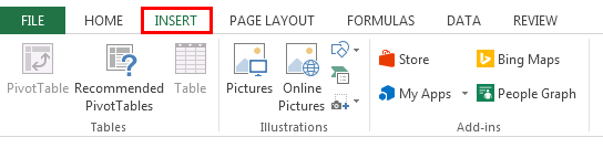
Step 1: Click on the “INSERT” Tab as highlighted in below image:
Step 2: Under the “Insert” tab, you will find “Shapes”, which is a part of the “Illustrations” group
Step 3: In “Shapes”, you will find a wide variety of lines from line to scribble that we will be used according to our requirement:
Purpose of Drawing a line in Excel
Below are a few scenarios that you may come across.
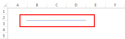
Example #1 – Draw a simple line
Step 1: Select “Line” from the “Lines” menu.
![]()
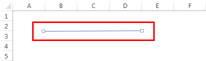
Step 2: Click anywhere in the document or the point from where you want to start, hold and drag your mouse pointer to a different location or the point where you want to end and then release.

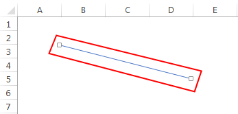
Step 3: In case you release the mouse cursor in between, you need not worry at all. Select the line, and you will see two dots at each end of the line as shown in below image:
Step 4: Select the dot from any end to resize the line or to change its direction, and you will get the output as shown below:
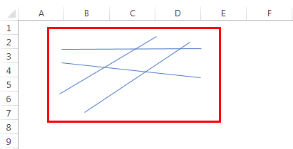
Example #2 – Draw multiple lines without selecting “line shape” again
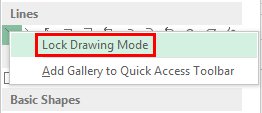
After the first line, if you need to create another line of the same type, you have to select the line again from the “Shapes” menu. What if we need to draw multiple lines without selecting them back from the “Shapes” menu. To overcome this situation, Excel has an inbuilt functionality, i.e. “Lock Drawing Mode”. Below are the steps that you need to follow to draw multiple lines repeatedly.
Step 1: While selecting the type of line, right-click on the required type and select “Lock Drawing Mode” as shown below:
Step 2: Click anywhere in the document or the point from where you want to start, hold and drag your mouse pointer to a different location or the point where you want to end and then release the mouse cursor.
Step 3: Repeat “Step 2” for every line you need to draw. After you have drawn the number of required lines, Press the “Esc” button.
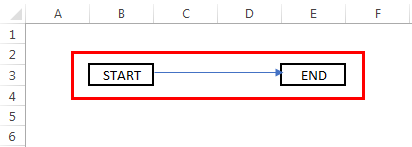
Example #3 – Draw an arrow in a flow diagram
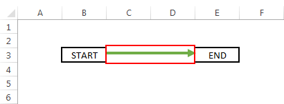
Imagine you need to create a flow diagram to explain the process or steps you follow for a certain project. In this situation, a simple line might not be useful as you need to specify the direction of the flow. We typically use “Line arrow” for such situations.
Below are the steps you need to take to draw it:
Step 1: Select “Line Arrow” from the “Lines” menu.
![]()
Step 2: Click anywhere in the document or the point from where you want to start, hold and drag your mouse pointer to a different location or the point where you want to end and then release the mouse cursor.
Example #4 – Format the line to make it more presentable
Sometimes we need to present our work to others in both the professional and personal world. One thing we should keep in mind is that we might have to make it look visually appealing according to the situation and all you need to do is follow the below set of steps:
Step 1: Select the line which you want to format.
Note: You can also select multiple lines to format them in the same manner in one go and avoid repeating the steps.
Step 2: Select the “Format” tab under the “Drawing Tools” as highlighted below:
Under the “Format tab”, you will have access to a lot of different options. You can change the color of the line or its width/thickness. You can even add some visual effects to it to make it more visually appealing.
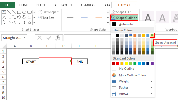
To format Color:
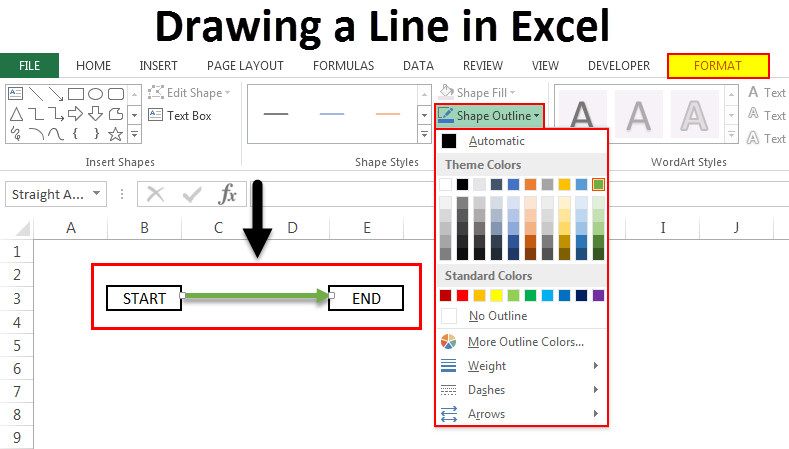
Step 3: Now, select “Shape Outline” from the “Format tab” and choose the desired color for your line.
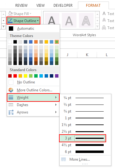
To format Size:
Step 3: Now, select “Shape Outline” from the “Format tab” and choose “Weight” and then the required width.
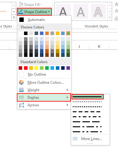
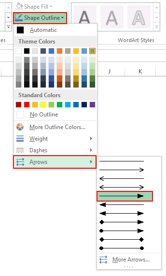
Similarly, under the “Shapes Outline”, you will find “Dashes” and “Arrows”, which can be used to make the line dotted or to change the direction or type of arrows.
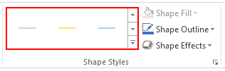
You can also use some pre-defined styles for a quick turnaround. They are available under the header “Shape Styles”, as shown below:
To format Shape effects:
Step 3: To add shape effects, select “Shape Effects” from the “Format tab”, and you will see a wide variety of effects that can be used.
Let us take an example of adding shadow to the line and see it looks like:
Step 4: Select “Shadow” from the “Shape Effects” menu as shown below:
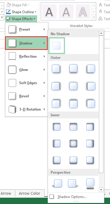
Step 5: Select the required effect from the “Shadow” menu, and you will see an output similar to the one shown below:
Things to Remember
This was an overview of drawing a line in excel and some of its applications. To draw other shapes and format them, all you need to do is select the required shape from the “Shapes” menu and follow the steps we used above to draw a line in excel. You make things look simple; the method of drawing a line in excel will be more helpful.
Some popular types of lines.
- Line
- Line Arrow
- Line Arrow: Double
- Connector: Elbow Arrow
- Connector: Elbow Double-Arrow
Some other applications.
- Used in charts to mark threshold values or as stat markers
- Used as dividers to segregate the spreadsheet into two or multiple regions.
Recommended Articles
This has been a guide to Drawing a line in Excel. Here we discuss Drawing a line in Excel and how to use Drawing a line in Excel along with practical examples and a downloadable excel template. You can also go through our other suggested articles –
- Data Table in Excel
- Combo Box in Excel
- Bubble Chart in Excel
- Scrollbar in Excel