
Excel for Microsoft 365 Excel 2021 Excel 2019 Excel 2016 Excel 2013 More…Less
You can square a number in Excel with the power function, which is represented by the carat ^ symbol. Use the formula =N^2, in which N is either a number or the value of the cell you want to square. This formula can be used multiple times throughout a worksheet.
Square a number in its own cell
Follow these steps:
-
Click inside a cell on your worksheet.
-
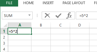
Type =N^2 into the cell, where N is the number you want to square. For example, to insert the square of 5 into cell A1, type =5^2 into the cell.

-
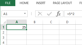
Press Enter to see the result.
Tip: You can also click into another cell to see the squared result.
Square a number in a different cell
Follow these steps:
-
Click inside a cell and type the number that you want to square.
-
Select another empty cell in the worksheet.
-
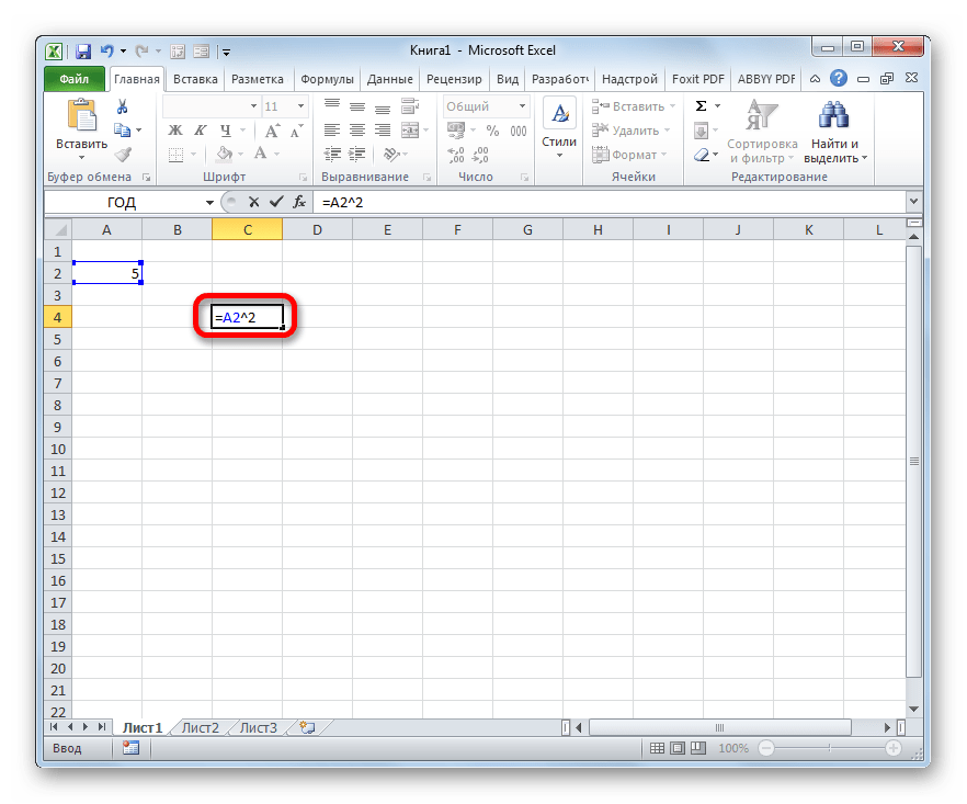
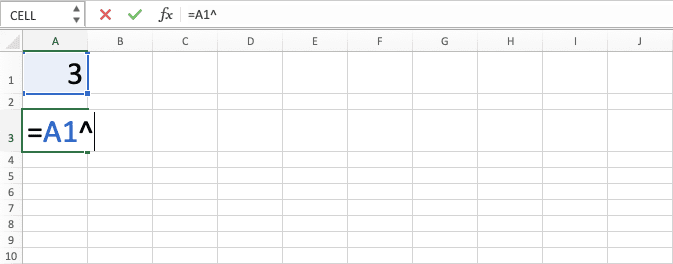
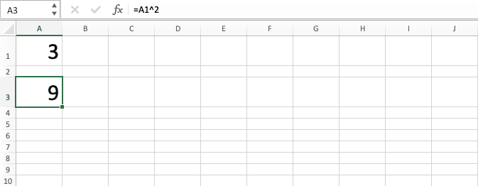
Type =N^2 into the empty cell, in which N is a cell reference that contains the numeric value you want to square. For example, to display the square of the value in cell A1 into cell B1, type =A1^2 into cell B1.
-
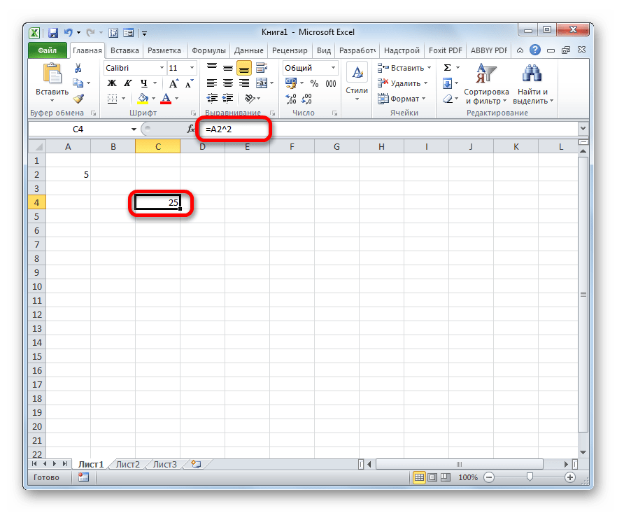
Press Enter to see the result.
Need more help?
You can always ask an expert in the Excel Tech Community or get support in the Answers community.
Need more help?
Want more options?
Explore subscription benefits, browse training courses, learn how to secure your device, and more.
Communities help you ask and answer questions, give feedback, and hear from experts with rich knowledge.
Square a number
- Click inside a cell on your worksheet.
- Type =N^2 into the cell, where N is the number you want to square. For example, to insert the square of 5 into cell A1, type =5^2 into the cell.
- Press Enter to see the result. Tip: You can also click into another cell to see the squared result.
Contents
- 1 How do you type 2 squared in Excel?
- 2 How do you square a shape in Excel?
- 3 How do you square a sheet?
- 4 How do you type a small 2?
- 5 How do you type 2 squared?
- 6 How do you square a number?
- 7 How do you square on Google?
- 8 How do you type 1 2 on a keyboard?
- 9 How do you write 2 cubed?
- 10 How do you type square root on a keyboard?
- 11 How do you write square roots?
- 12 Can you open sheets in Excel?
- 13 How do you write two and a half?
- 14 What is another way to say 1 2?
How do you type 2 squared in Excel?
To type the 2 Squared Symbol anywhere on your PC or Laptop keyboard (like in Microsoft Word or Excel), press Option + 00B2 shortcut for Mac. And if you are using Windows, simply press down the Alt key and type 0178 using the numeric keypad on the right side of your keyboard.
How do you square a shape in Excel?
Add a shape in Excel, Outlook, Word, or PowerPoint
- On the Insert tab, click Shapes.
- Click the shape you want, click anywhere in the workspace, and then drag to place the shape. To create a perfect square or circle (or constrain the dimensions of other shapes), press and hold Shift while you drag.
How do you square a sheet?
To square numbers in Google Sheets, type a numbers or a cell reference (to a cell containing a number), then type a carrot “^”, then type the number “2”, and then press enter. Here are a couple examples of squaring formulas: =10^2.
How do you type a small 2?
Hold down Alt and key in 0178 and let go of Alt. A superscript 2 will appear. Incidentally, if you needed ‘cubed’ instead of ‘squared’ then type 0179 and you’ll get a superscript 3. In fact, this will work anywhere in Windows or online – even in Word.
How do you type 2 squared?
Inserting the squared symbol on your Android smartphone is relatively easy and straightforward. To insert the squared sign, just long-press the number 2 and it will insert the superscript ².
How do you square a number?
Want to square a number? Just take the number and multiply it by itself! If you square an integer, you get a perfect square!
How do you square on Google?
How Do You Write Squared on Google Docs?
- Open a Google Docs document.
- Type “2” next to the number you want to square and highlight it.
- In the horizontal toolbar at the top of the screen, click “Format.”
- Place your cursor over “Text.”
- Click “Superscript.”
How do you type 1 2 on a keyboard?
Some fractions (1/4, 1/2, and 3/4) automatically switch to a fraction character when you type them (¼, ½, ¾). But others do not (1/3, 2/3, 1/5, etc.). To switch to a fraction character, click Insert > Symbols > More Symbols. In the Subset drop-down list, click Number Forms and select a fraction.
How do you write 2 cubed?
2 cubed is 23 = 2×2×2 = 8. The term “cube” can be remembered because there are three dimensions in a cube (height, width, and depth) and the number being cubed appears three times in the calculation.
How do you type square root on a keyboard?
To type the square root symbol using your keyboard, hold down the Alt key and then type 251 on the numeric keypad. The result is this: √.
How do you write square roots?
A square root is written with a radical symbol √ and the number or expression inside the radical symbol, below denoted a, is called the radicand. To indicate that we want both the positive and the negative square root of a radicand we put the symbol ± (read as plus minus) in front of the root.
Can you open sheets in Excel?
Google Sheets allows you to download your spreadsheets in a format that can be opened in Microsoft Excel.
How do you write two and a half?
Mixed numbers have a whole number followed by the fraction (2 1/2). You would say “two and one half.” The other format is an improper fraction where the numerator is greater than the denominator (5/2).
What is another way to say 1 2?
We pronounce 1/2 as one-half, 1/4 as one-quarter, and 3/4 as three-quarters.
Содержание
- Square a number
- Square a number in its own cell
- Square a number in a different cell
- Need more help?
- Square a number
- Square a number in its own cell
- Square a number in a different cell
- Need more help?
- Возведение числа в квадрат в Microsoft Excel
- Процедура возведения в квадрат
- Способ 1: возведение с помощью формулы
- Способ 2: использование функции СТЕПЕНЬ
- How to Make a Square Excel Calculation and All Its Formulas & Functions
- How to Write a Square Excel Calculation With the ^ Symbol
- How to Write a Square Excel Calculation With the * Symbol
- How to Make a Square Excel Calculation With the POWER Formula
- Exercise
- Questions
- Additional Note
Square a number
You can square a number in Excel with the power function, which is represented by the carat ^ symbol. Use the formula =N^2, in which N is either a number or the value of the cell you want to square. This formula can be used multiple times throughout a worksheet.
Square a number in its own cell
Follow these steps:
Click inside a cell on your worksheet.
Type =N^2 into the cell, where N is the number you want to square. For example, to insert the square of 5 into cell A1, type =5^2 into the cell.
Press Enter to see the result.
Tip: You can also click into another cell to see the squared result.
Square a number in a different cell
Follow these steps:
Click inside a cell and type the number that you want to square.
Select another empty cell in the worksheet.
Type =N^2 into the empty cell, in which N is a cell reference that contains the numeric value you want to square. For example, to display the square of the value in cell A1 into cell B1, type =A1^2 into cell B1.
Press Enter to see the result.
Need more help?
You can always ask an expert in the Excel Tech Community or get support in the Answers community.
Источник
Возведение числа в квадрат в Microsoft Excel

Одним из наиболее частых математических действий, применяемых в инженерных и других вычислениях, является возведение числа во вторую степень, которую по-другому называют квадратной. Например, данным способом рассчитывается площадь объекта или фигуры. К сожалению, в программе Excel нет отдельного инструмента, который возводил бы заданное число именно в квадрат. Тем не менее, эту операцию можно выполнить, использовав те же инструменты, которые применяются для возведения в любую другую степень. Давайте выясним, как их следует использовать для вычисления квадрата от заданного числа.
Процедура возведения в квадрат
Как известно, квадрат числа вычисляется его умножением на самого себя. Данные принципы, естественно, лежат в основе вычисления указанного показателя и в Excel. В этой программе возвести число в квадрат можно двумя способами: использовав знак возведения в степень для формул «^» и применив функцию СТЕПЕНЬ. Рассмотрим алгоритм применения данных вариантов на практике, чтобы оценить, какой из них лучше.
Способ 1: возведение с помощью формулы
Прежде всего, рассмотрим самый простой и часто используемый способ возведения во вторую степень в Excel, который предполагает использование формулы с символом «^». При этом, в качестве объекта, который будет возведен в квадрат, можно использовать число или ссылку на ячейку, где данное числовое значение расположено.
Общий вид формулы для возведения в квадрат следующий:
В ней вместо «n» нужно подставить конкретное число, которое следует возвести в квадрат.
Посмотрим, как это работает на конкретных примерах. Для начала возведем в квадрат число, которое будет составной частью формулы.
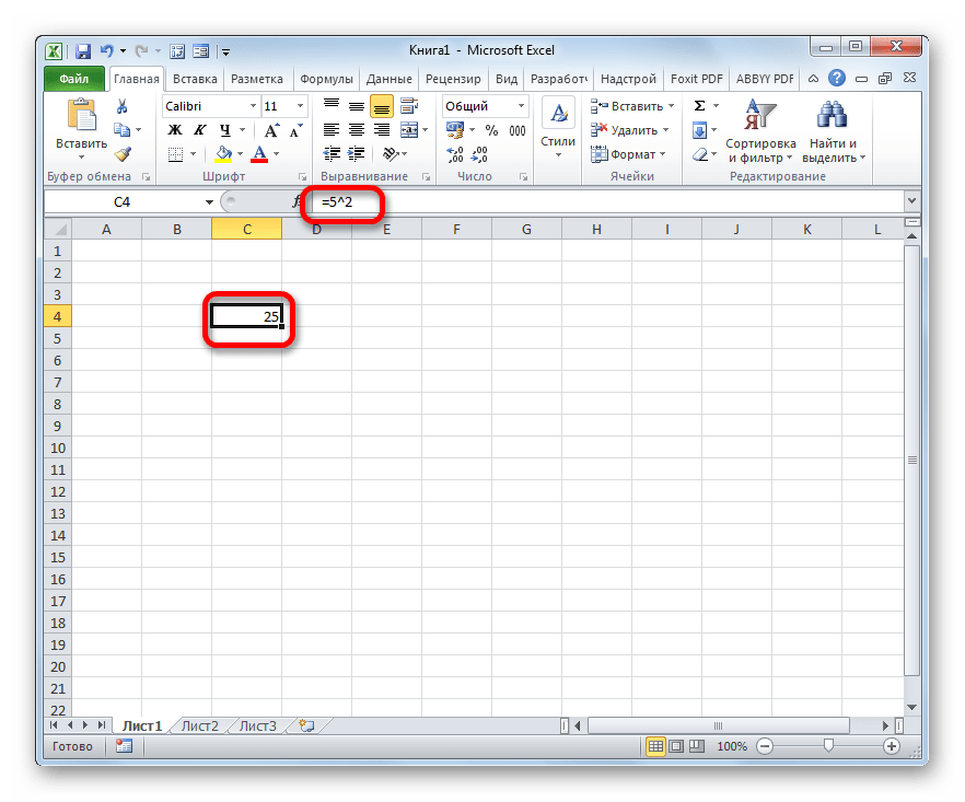
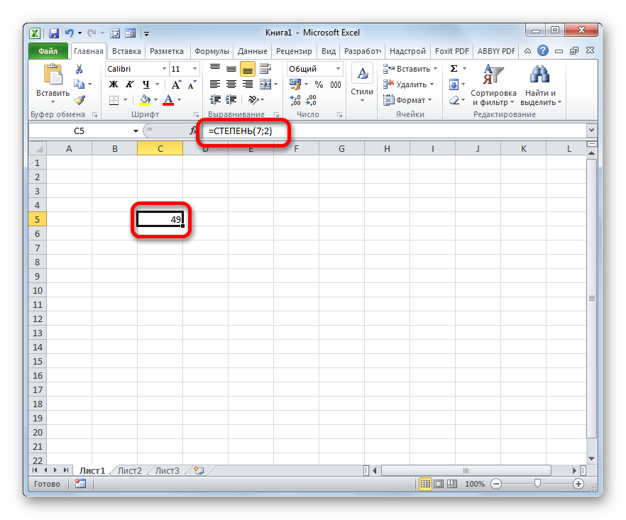
- Выделяем ячейку на листе, в которой будет производиться расчет. Ставим в ней знак «=». Потом пишем числовое значение, которое желаем возвести в квадратную степень. Пусть это будет число 5. Далее ставим знак степени. Он представляет собой символ «^» без кавычек. Затем нам следует указать, в какую именно степень нужно произвести возведение. Так как квадрат – это вторая степень, то ставим число «2» без кавычек. В итоге в нашем случае получилась формула:
=5^2 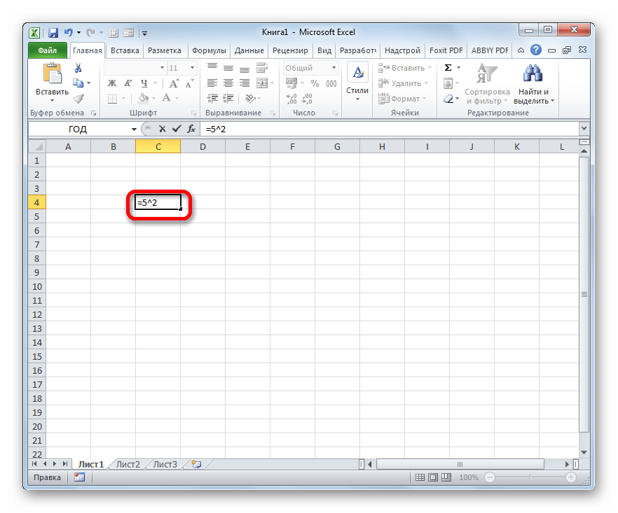
Теперь давайте посмотрим, как возвести в квадрат значение, которое расположено в другой ячейке.
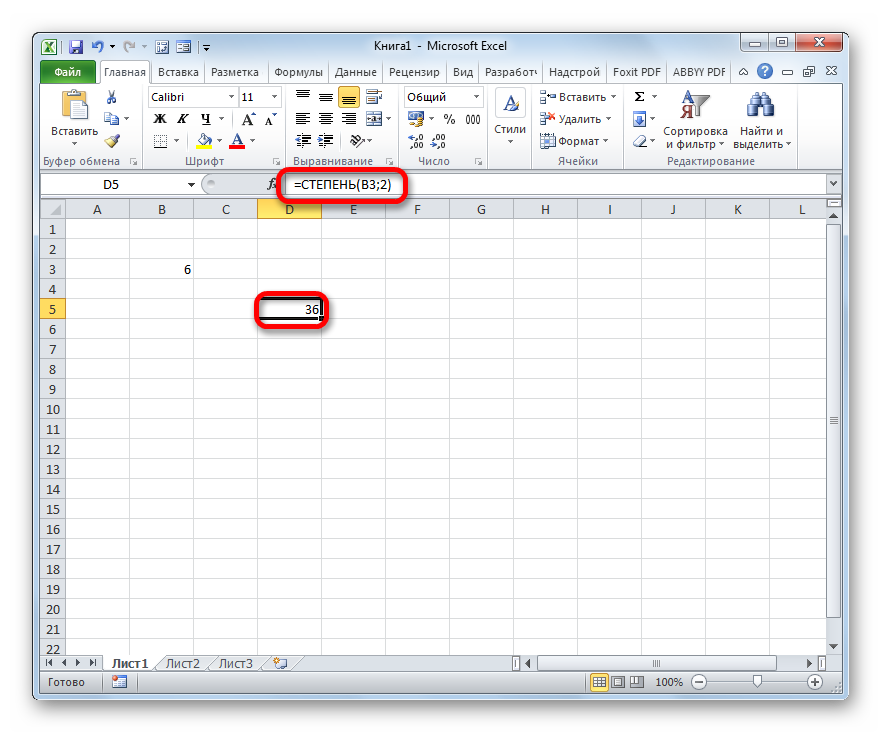
- Устанавливаем знак «равно» (=) в той ячейке, в которой будет выводиться итог подсчета. Далее кликаем по элементу листа, где находится число, которое требуется возвести в квадрат. После этого с клавиатуры набираем выражение «^2». В нашем случае получилась следующая формула:
Способ 2: использование функции СТЕПЕНЬ
Также для возведения числа в квадрат можно использовать встроенную функцию Excel СТЕПЕНЬ. Данный оператор входит в категорию математических функций и его задачей является возведение определенного числового значения в указанную степень. Синтаксис у функции следующий:

Аргумент «Число» может представлять собой конкретное число или ссылку на элемент листа, где оно расположено.
Аргумент «Степень» указывает на степень, в которую нужно возвести число. Так как перед нами поставлен вопрос возведения в квадрат, то в нашем случае данный аргумент будет равен 2.
Теперь посмотрим на конкретном примере, как производится возведение в квадрат с помощью оператора СТЕПЕНЬ.
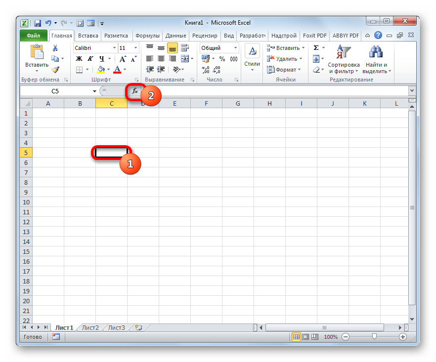
- Выделяем ячейку, в которую будет выводиться результат расчета. После этого щелкаем по иконке «Вставить функцию». Она располагается слева от строки формул.
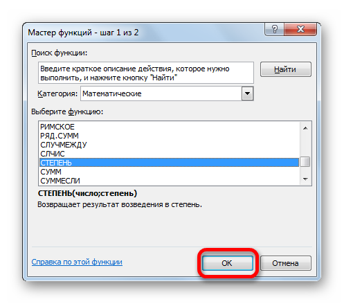
- Происходит запуск окошка Мастера функций. Производим переход в нем в категорию «Математические». В раскрывшемся перечне выбираем значение «СТЕПЕНЬ». Затем следует щелкнуть по кнопке «OK».
- Производится запуск окошка аргументов указанного оператора. Как видим, в нем располагается два поля, соответствующие количеству аргументов у этой математической функции.
В поле «Число» указываем числовое значение, которое следует возвести в квадрат.
В поле «Степень» указываем цифру «2», так как нам нужно произвести возведение именно в квадрат.
После этого производим щелчок по кнопке «OK» в нижней области окна. 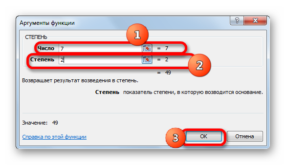
Также для решения поставленной задачи вместо числа в виде аргумента можно использовать ссылку на ячейку, в которой оно расположено.
- Для этого вызываем окно аргументов вышеуказанной функции тем же способом, которым мы это делали выше. В запустившемся окне в поле «Число» указываем ссылку на ячейку, где расположено числовое значение, которое следует возвести в квадрат. Это можно сделать, просто установив курсор в поле и кликнув левой кнопкой мыши по соответствующему элементу на листе. Адрес тут же отобразится в окне.
В поле «Степень», как и в прошлый раз, ставим цифру «2», после чего щелкаем по кнопке «OK». 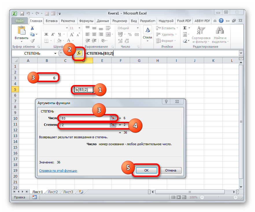
Как видим, в Экселе существует два способа возведения числа в квадрат: с помощью символа «^» и с применением встроенной функции. Оба этих варианта также можно применять для возведения числа в любую другую степень, но для вычисления квадрата в обоих случаях нужно указать степень «2». Каждый из указанных способов может производить вычисления, как непосредственно из указанного числового значения, так применив в данных целях ссылку на ячейку, в которой оно располагается. По большому счету, данные варианты практически равнозначны по функциональности, поэтому трудно сказать, какой из них лучше. Тут скорее дело привычки и приоритетов каждого отдельного пользователя, но значительно чаще все-таки используется формула с символом «^».
Источник
How to Make a Square Excel Calculation and All Its Formulas & Functions


In this tutorial, we will discuss completely how to make a square excel calculation on a number. All formulas/functions we can use to calculate square in excel will also be explained here.
One calculation we often do when processing numbers is square/the power of two. If we often use excel as a tool to process our numbers, then understanding the way to square there becomes important.
Generally, the method to write a square formula in excel can be divided into three. They are the manual writing with the ^ symbol, manual writing with the * symbol, and the POWER formula. We will talk in the next parts about the general writing form for each, example, and their writing steps in detail.
Disclaimer: This post may contain affiliate links from which we earn commission from qualifying purchases/actions at no additional cost for you. Learn more
Want to work faster and easier in Excel? Install and use Excel add-ins! Read this article to know the best Excel add-ins to use according to us!
How to Write a Square Excel Calculation With the ^ Symbol
Now, we will discuss the first method to do a square excel calculation, which is by using the ^ symbol.
The caret symbol (^) is a power calculation symbol in excel formula writing. Because the square is the same as the power of 2, we can use it to get a square calculation result.
Generally, here is the writing to calculate a square in excel with the ^ symbol.
The number there is the number you want to square/power by 2 in excel. The number input in the formula can be typed or inputted through the media of a cell coordinate.
We use ^ in the writing as a power symbol and 2 as the power factor. We use 2 there because what we look for is the square or the power of 2 from our number.
Write that writing form correctly in your cell and enter. You will immediately get the square result of your number!
To make it clearer about the writing, see its implementation example in excel below.

You can see the writing example in the screenshot’s formula bar. We get the square of all the numbers on the left using that form of writing.
To make you understand further about this method to write a square formula, we will give the detailed writing steps here. We will explain each step with the help of a screenshot to make you understand it easier.
- Type an equal sign ( = ) in the cell where you want to put the square result of your number

Input the number to be squared or the cell coordinate where it is after =. Type a caret symbol ( ^ ) after that
Type 2

How to Write a Square Excel Calculation With the * Symbol
There is another method for us to write a square calculation formula in excel. That method is using the help of the * symbol.
As we know, the power calculation is the same as multiplying a number with the number itself. Because of that, we can multiply our number with its own value to get its square result in excel.
The symbol that represents multiplication in excel is the star symbol or *. Therefore, we can square our number by using the * symbol in the writing that we do.
Generally, here is the writing form of a square formula in excel with the * symbol.
The number there is the number we want to square in our data processing.
To make it clearer about this square formula writing with the * symbol, here is its implementation example in excel.
As we can see in the screenshot’s formula bar, the writing in the example uses the form explained earlier. Write the multiplication formula correctly and you can get the square result of your number easily!
To add your understanding about this method’s application, here is the step-by-step of its writing in detail.
- Type an equal sign ( = ) in the cell where you want to put the square result of your number
Input the number to be squared or the cell coordinate where it is after =. Type a star symbol ( * ) after that
Input the number or the cell coordinate again
How to Make a Square Excel Calculation With the POWER Formula
What if we want to use a built-in formula available in excel to square our number? This can be done by using the POWER formula.
POWER is made by excel to calculate the power of a number in our worksheet. The inputs it needs are the number we want to power and the power factor. By inputting 2 in its power factor input, we can get the square result of our number using this formula.
Generally, here is the writing form of POWER so we can get our square calculation result from it.
Don’t forget to input 2 in the power factor input part so you can get the correct result.
The implementation example of the writing in excel is as follows.
As you can see, POWER can be used to do your number’s square calculation. Give your inputs correctly and you can get your result fast!
To add to your understanding of this method, here are the writing steps.
- Type an equal sign ( = ) in the cell where you want to put the result in

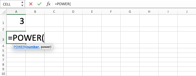
Type POWER (can be with large and small letters) and an open bracket sign after =
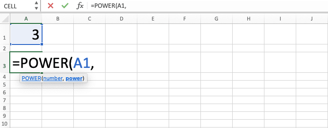
Input the number to be squared or the cell coordinate where it is after the open bracket sign. Then type a comma sign ( , )
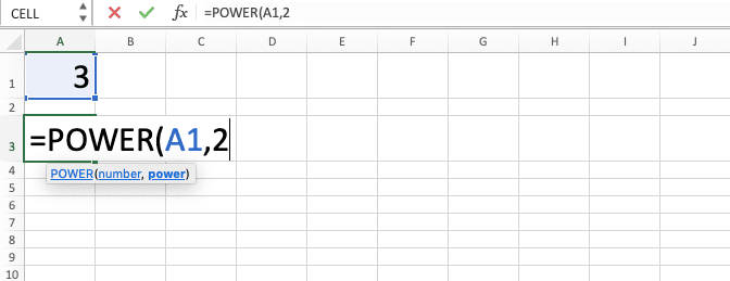
Type 2
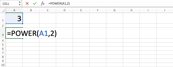
Type a close bracket sign

Exercise
After learning the methods to write a square formula in excel, now let’s do an exercise. This is so you can deepen your understanding of those methods.
Download the following exercise file and answer all the questions. Download the answer key file if you have finished the exercise and want to check your answers. Or probably when you are confused about how to answer the questions.
Link to the exercise file:
Download here
Questions
- What is the final score of each person? Use the ^ symbol method to find the answer!
- What is the final score of each person? Use the * symbol method to find the answer!
- What is the final score of each person? Use the POWER formula method to find the answer!
Link to the answer key file:
Download here
Additional Note
To do the power calculation with other factors besides 2, you can learn it by visiting this Compute Expert tutorial.
Related tutorials you should learn:
Источник
Thanks to spreadsheet software like Excel, it has become easier than ever to find squares of thousands of numbers at a time, even if some of them are quite large.
With Excel there are two ways in which you can square a number:
- Using a Formula
- Using a Function
Both ways are quick and easy, as you will soon see.
In this tutorial, we are going to show you how to use the above two ways to find the square of a number in Excel.
Two Quick Ways to Square a Number in Excel
To understand how to quickly square numbers in Excel, we are going to use the following dataset:

In this dataset, we want to find the square of each value of column A and display the result in column B.
Let us see how to accomplish this in Excel.
Using a Formula to Square a Number
Squaring a number simply means multiplying a number by itself, or raising it to the power of 2.
So, to square the number in the cell reference A2, you can write the formula in two different ways:
- Using the multiplication operator to multiply it by itself
- Using the caret operator to raise the number to the power of 2
Using the Multiplication Operator
In Excel, you can multiply numbers using the multiplication operator, also known as an asterisk symbol (‘*’).
So to multiply the value in cell A2 with itself, you can use the formula:
=A2 * A2
Thus, here are the steps you can follow to find the square of each number in our given dataset:
- Select the cell where you want the first result to appear (cell B2).
- Type the formula: =A2*A2.
- Press the return key.
- The square of the value in A2 should now be displayed as the result in cell B2.

- Drag down the fill handle (the small square at the bottom right corner of cell B2) till you reach the last row of your dataset.
- Each cell in column B should now contain the square of the corresponding value in column A.


Using the Caret Operator
In Excel, you can raise one number to the power of another using the exponent operator, also known as a caret symbol (‘^’).
So to square the value in cell A2 you need to raise it to the power of 2. For this, you can use the formula:
=A2 ^ 2
Thus, here are the steps you can follow to find the square of each number in our given dataset:
- Select the cell where you want the first result to appear (cell B2).
- Type the formula: =A2^2.
- Press the return key.
- The square of the value in A2 should now be displayed as the result in cell B2.

- Drag down the fill handle (the small square at the bottom right corner of cell B2) till you reach the last row of your dataset.
- Each cell in column B should now contain the square of the corresponding value in column A.
Using a Function to Square a Number
Excel provides a useful function to raise a number to a certain power.
The POWER function works like an exponent in a standard math equation and raises one number to the power of another.
The syntax for the POWER function is as follows:
=POWER (number, power)
Here,
- number is the number that you want to raise to an exponent.
- power is the exponent you want to raise the number to the power of.
So if you want to use the POWER function to find the square of a number, say the value in cell A2, you need to raise it to the power of 2 as follows:
=POWER(A2,2)
Thus, here are the steps you can follow to find the square of each number in our given dataset:
- Select the cell where you want the first result to appear (cell B2).
- Type the formula: =POWER(A2,2).
- Press the return key.
- The square of the value in A2 should now be displayed as the result in cell B2.

- Drag down the fill handle (the small square at the bottom right corner of cell B2) till you reach the last row of your dataset.
- Each cell in column B should now contain the square of the corresponding value in column A.

Note: The POWER function is located along with the Math & Trig functions in the Formulas tab (under Function Library). If you’re in the Insert Function dialog box, you can find it under the Select a Category drop-down list.

In this tutorial, we showed you three very easy and quick ways to square a number in Excel.
The first two methods use a formula, while the third method uses the POWER function. We hope you found this tutorial simple and easy to follow.
Other Excel tutorials you may also like:
- How to Insert Square Root Symbol in Excel
- How to Subtract Multiple Cells from One Cell in Excel
- How to Calculate Standard Error In Excel
- How to Use e in Excel | Euler Number in Excel
- How to Use Pi (π) in Excel
- How to Calculate Antilog in Excel
- How to Find Range in Excel
- How to Calculate Nth Root in Excel?
Squaring a number multiplies that number by itself. Let’s learn how to square numbers in Microsoft Excel with these easy steps.
Squaring a number multiplies that number by itself. It’s a powerful function, and it’s easy to calculate in Excel. Let’s learn how to square numbers in Microsoft Excel.
Excel offers two quick ways to find a square. With one, you input the number and then square it. With the other, you can find the square of numbers that are already in your workbook. We’ll learn how to do both.
How to Find a Square in Microsoft Excel
Let’s say you want to square the number 10. Of course, you could simply multiply 10 x 10. But Excel can square a number with a simple formula instead.
Click into any cell, and type =10. Then, type a caret symbol, ^. Finally, type 2.

Your finished formula is:
=10^2
Hit Enter on your keyboard, and Excel will square 10 and return the value 100.

(Hint: If you need to raise a number to a higher power, repeat the same steps, but change the 2 to a 3, 4, or other value).
How to Square an Existing Number in Microsoft Excel
Imagine that you already have a number in Excel, and you want to square it. There’s no need to type it over again in a formula like the one above.
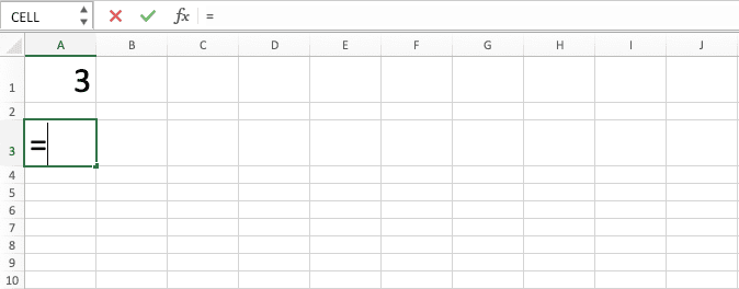
To square an existing number, click into a blank cell. Type = again. Now, you’ll want to click on the cell containing the number you want to square. In this case, that’s cell A1.
Now, type ^2 and hit Enter. Excel returns your solution: 900.

You can even perform this step with a list of numbers, by simply clicking and dragging your formulas into an adjacent empty column or row.
As you can see, Excel offers plenty of great ways to quickly square numbers. They save you time and ensure your calculations are always accurate.
The aim is simple. Squaring a number, a number raised to the power 2, the number multiplied by itself; it’s all the same thing, you know the drill. If this is giving you unfond memories of your childhood math classes, it’s a good thing you’re here because we aren’t going to math-splain you.
This tutorial is about squaring a number in Excel, and we will break down all the methods mentioned above. Throughout this tutorial, for our examples, we will square the numbers in one column and try to print the results next to them using different easy peasy ways.
Let’s start diving into the easy peasy ways which we will split into 2 sections; in the first section, we will square numbers using formulas and in the second section, we will use functions.
 1")
Squaring Numbers Using Formulas
In this section, we will use two formulas to square numbers:
- Formula using multiplication operator
- Formula using caret operator
Let’s see them one by one.
Multiplication Operator Based Formula For Squaring Numbers
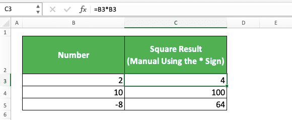
By multiplication operator, we are referring to the asterisk ( * ) symbol. A squared number is basically the number multiplied by itself so we will do just that on our worksheet in the form of a formula. Let’s see this practically.
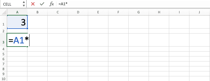
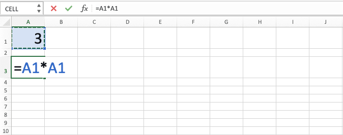
We will use the following formula in our example:
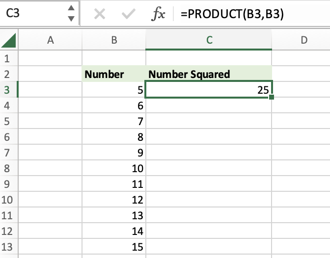
=B3*B3 //where B3 contains the number to be squared
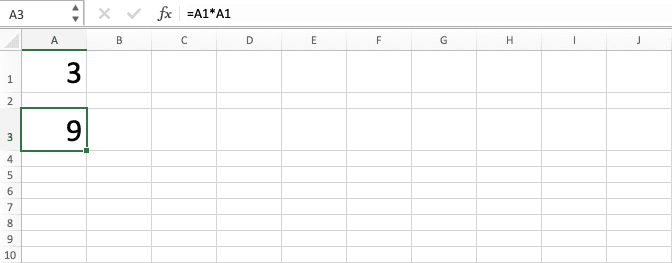
This reads as B3 multiplied by B3. The value in cell B3 is 2 and so the calculation goes as 2 multiplied by 2. Here is the outcome:
 2")
Also, instead of making use of the cell references, you can apply the formula directly as:
=2*2 //returns 4
Wasn’t that easy breezy? It’s nice to have Excel do all the work for you. Let’s keep flowing with the easy breeze into the next formula.
Caret Operator Based Formula For Squaring Numbers
By caret operator, we are referring to the » ^ » symbol. Caret Operator is also known as Exponent operator. Does anyone remember five raised to the power two?
(Hint: Math classes again)
The caret is essentially saying ‘raised to the power’. Hence, 5 raised to the power 2 becomes 5^2, squaring the number 5. Let’s see how it helps us in Excel.
Referring to our example, the formula using the caret symbol to square a number will be:
=B3^2 //where B3 contains the number to be squared
This reads as B3 raised to the power 2. The value in cell B3 is 2 and so the calculation goes as 2 raised to the power 2 with «4» as the squared result. Applying this formula to square numbers will give us the following results:
![]()
Also, instead of relying on the cell references, you can apply the formula directly as:
=2^2 //returns 4
Just now, we used a formula to raise the power of a number. We can apply the same principle using a function, which brings us to our next section where we square numbers using functions.
Recommended Reading: Calculate Square Root of a Number
Squaring Numbers Using Excel Functions
This section covers the use of functions to square numbers. The functions we will use are:
- The POWER function
- The PRODUCT function
- The SUMPRODUCT function
Using POWER Function
The POWER function works like a caret operator, raising the number to a power. The syntax of POWER function is very simple it takes two arguments: number and power.
For the purpose of this article, we are interested in squaring the number so we are working only with raising the numbers to the power «2». The POWER function can easily do that for us.
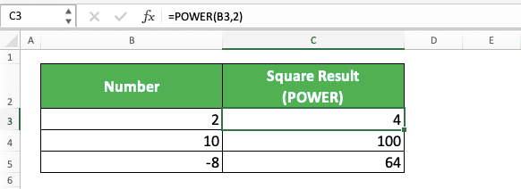
This is how we will use the POWER function for our example:
=POWER(B4, 2) //where B4 contains the number to be squared
The value in cell B4 is «10». The «2» in the second argument here is the power by which the number in cell B4 («10») is to be raised. The result of 10 raised to the power 2 is 100 which we have in our results:
 4")
For instances where you wish to skip the cell reference in the function, you can apply the function directly as:
=POWER(10,2) //returns 100
Using PRODUCT Function
The PRODUCT function will multiply all the numbers given as arguments. Similar to how we used a multiplication formula to multiply the number with itself, we can use the PRODUCT function for the same calculation, separating the numbers by commas instead of asterisks (*).
Carrying down our base example, for squaring a number, we will need to supply the number twice in the formula and that should do it:
=PRODUCT(B4, B4) //where B4 contains the number to be squared
Cell B4 contains the number «10». Since the PRODUCT function multiplies all the supplied numbers, for squaring the number 10, we only need to supply it twice to the formula. 10 multiplied by 10 gives us 100 which we also have here in the results:
 5")
For instances where you wish to skip the cell reference in the function, you can apply the function directly as
=PRODUCT(10,10) //returns 100
Similar to the PRODUCT function, we can use the SUMPRODUCT function for squaring numbers. Let’s see ahead.
Using SUMPRODUCT Function
An extension of the PRODUCT function, the SUMPRODUCT function multiplies the supplied number groups and then adds the outcomes of the multiplied groups for the final result. It works like this:
For instance, if we have a SUMPRODUCT function as:
=SUMPRODUCT(A1:A3,B1:B3)
Then the result will be calculated as –
The SUMPRODUCT function will multiply each element from both the cell ranges and then added them to one another to return the final result.
Mathematically this is equivalent to writing –
(A1*B1) + (A2*B2) + (A3*B3)
Now, lets jump back to our case –
For squaring a number we need to multiply the number by itself. Therefore, we only need to pass one group of numbers to the SUMPRODUCT function. SUMPRODUCT will multiply that for us and hand us the result. We are to use it just like the PRODUCT function.
So if we are to use it exactly like the PRODUCT function, why add the «SUM» prefix? Well, since we are exploring options and this is viable, we have to have the talk about it. Let’s put it to use with our example.
=SUMPRODUCT(B4,B4) //where B4 contains the number to be squared
Cell B4 contains the number «10». As the SUMPRODUCT function multiplies all the supplied number groups and then adds the result of those multiplied groups, we will only provide one number group i.e. «B4, B4» which will be «10, 10» since that is what we require for squaring the number.
SUMPRODUCT will multiply 10 by 10. The result will be 100. Since there is no other number group to multiply, the final outcome of SUMPRODUCT is 100.
 6")
For instances where you wish to skip the cell reference in the function, you can apply the function directly as:
=SUMPRODUCT(10,10) //returns 100
This ends our tutorial, fair and square. Thanks to the power of Excel, we have many options for the simplest of calculations. There’s so much more to explore and this is just a wodge of Excel. We’ll come up with another wodge soon, be sure to have your part!
Home / Excel Formulas / How to Square a Number in Excel
If you want to square a number in Excel, you can use two easy ways to follow methods, and both methods work in the same way. You need to specify the number for which you want to calculate the square and specify 2 as you want to calculate the square.
Ahead in this tutorial, we will use an example to understand it.
Using POWER to Calculate Square
- Enter the POWER function in the cell.
- Refer to the cell where you have the number for which you need to calculate the square.
- In the second argument, enter 2 as you need to raise the power to 2.
- Close the function and hit enter.

The moment you need to hit enter the function returns the square as you can see in the above example.
Using the Power Operator (^)
In the same way, you also use the power operator (^) to get the square of a number in Excel. And in this method, you don’t need to use any function. Here’s the method:
- Refer to the cell where you have a number for which you want to calculate the square.
- Enter a ^ using the keyboard (you can find it on the number key 6).
- Type 2, which tells Excel to raise its power to 2.
- Hit enter to get the result.

As I said, both functions work in the same way and are quite easy to use. But you can choose one according to your need.
More Formulas
- Calculate Compound Interest in Excel
- Calculate Cube Root in Excel
- Calculate Percentage Variance (Difference)
- Calculate Simple Interest in Excel
- Calculate SQUARE ROOT in Excel
- Calculate the Weighted Average in Excel
- Does Not Equal Operator in Excel
- Round a Number to Nearest 1000, 100, and 10
- Round to Nearest .5, 5. 50 (Down-Up) in Excel
- Round a Number to Nearest 1000 in Excel
- Add-Subtract Percentage from a Number
- Average But Ignore Errors
- Average Number but Exclude Zeros
- Average Only Non-Blank Cells
- Calculate the Average of the Percentage Values
- Calculate the Average of the Time Values
- Calculate the Cumulative Sum of Values
- Round Percentage Values
⇠ Back to 100+ Excel Formulas List (Basic + Advanced)
Are you looking for a way to square a number?
If you work in a field like carpentry, engineering, architecture, or technology, you probably are!
Squaring a number is the mathematical operation of multiplying a number by itself. As an example, a square-sized bedroom measuring 10 feet wide and 10 feet long could be expressed as 100 square feet by multiplying 10 by 10.
This post explores all the different ways to square a number in Microsoft Excel.
Square a Number with the Multiplication Operator
The most straightforward way to square a number is to multiply it by itself using the traditional multiplication operator.
= B3 * B3The above formula will multiply the number in cell B3 by itself. The asterisk (*) is the operator for multiplication.
You’ve just squared your number from cell B3!
To apply your formula to your other numbers, hover over the lower-right corner of the formula’s cell until your cursor turns to a plus (+), then double-click.
Square a Number with the Carat Operator
The carat operator (^) in Excel is designed for the specific operation of raising a number to a given power such as a square.
= B3 ^ 2To implement the carat operator on your number in cell B3, select an empty cell and paste the above formula into the formula bar.
The above value 2 following the carat operator is called the exponent of your number. Specifying 2 as your exponent will square the number.
Your number has been squared!
Hover the cursor over the active cell fill handle and double-click to fill the formula down.
Square a Number with the POWER Function
The POWER function is an expert way to calculate a number involving an exponent.
= POWER( B3 , 2 )To square your number from cell B3 using the POWER function, select an empty cell and paste the above formula into the formula bar.
The second argument is 2. This is the exponent of your number, so always specify 2 here for squaring.
Press Enter when done and see how your number gets squared!
To apply your formula to your other numbers, hover over the lower-right corner of the formula’s cell until your cursor turns to a plus (+), then double-click.
Square a Number with the PRODUCT Function
The PRODUCT function provides general multiplication of values in Excel. Because squaring is just a specific case of multiplication, you can use PRODUCT to square your number.
= PRODUCT( B3 , B3 )To use PRODUCT against your number in cell B3, select an empty cell and paste the above formula into the formula bar.
Your cell B3 is specified twice in the above formula because you’d like to multiply the B3 number by itself.
Press Enter to calculate the square of your number!
Double-click on the active cell fill handle to copy and paste the formula down your column.
Square a Number with the SUMSQ Function
Though the SUMSQ function is generally used for the summation of squared numbers, its summation feature is optional, leaving you the ability to simply square a single number.
= SUMSQ( B3 )To leverage SUMSQ for a number in cell B3, select an empty cell and paste the above formula into the formula bar.
You only need to provide your value from the cell B3 and SUMSQ will square it.
Press Enter and behold your squared number!
Double-click on the fill handle to copy down the formula.
Square a Number with Paste Special
Excel has a paste special feature that allows you to multiply copied numbers.
To square numbers using this feature, you copy your numbers to the clipboard, then paste over it with an instruction to multiply it by the clipboard contents.
Here’s how it works for a range of numbers.
- Select your range of numbers.
- Copy your numbers to the clipboard by selecting Copy under the Home ribbon tab or press Ctrl + C.
- While your number range is still selected, go to the Home ribbon tab, drop down the Paste menu and select Paste Special.
Alternatively, you can simply press Ctrl + Alt + V.
This will open the Paste Special menu.
- Select Multiple from the Paste Special dialog.
- Click on the OK button.
Each number in your selected range has now been squared!
Square a Number with Power Query
Power Query is a powerful data transformation tool for Excel table data.
Once your numbers are arranged in a table, you can create a query that dynamically squares your numbers by using a Power Query formula.
Follow these steps to get started.
- Select your range of numbers, including the column header.
- Select From Table/Range under the Data ribbon tab.
- At the Create Table prompt, click OK to convert your range into a table.
- Go to the Transform ribbon tab in the Power Query Editor.
- Click on the Scientific menu in the Numbers Column.
- Select the Power submenu.
- Select the Square option.
Your numbers have now been squared!
You can then place the squared numbers on your sheet.
- Under the Home ribbon tab, drop down the Close & Load menu and select Close & Load To.
- Choose a destination for your results. For example, choose the Existing worksheet starting at cell D2.
- Click OK.
Now your squared numbers appear as a range alongside your original numbers!
Square a Number with VBA
VBA is the code responsible for automating tasks in Excel.
If you’d like to square numbers in a range based on what is currently selected, VBA would be a good way to do that.
Here’s how to explore this option.
- First ensure that you see the Developer ribbon tab, since it may be hidden by default.
- Go to the Developer ribbon tab.
- Click Visual Basic or simply press Alt + F11.
- From the Visual Basic editor select the Insert menu.
- Select the Module menu item.
Sub SquareNumbers()
Dim selectedRange As Range
Set selectedRange = Application.Selection

For Each cell In selectedRange.Cells
    If Len(cell.Value) > 0 Then
        cell.Value = cell.Value * cell.Value
    End If
Next cell
End Sub
- In the new module window, paste the above VBA code.
The code will retrieve each cell in the currently-selected range selectedRange.
The cell’s value will get updated to a multiple of itself, effectively squaring the number. The Len() function is used to skip blank cells to which squaring does not apply.
- To run your code, go back to your sheet and select your range of numbers.
- Under the View ribbon tab, select Macros.
- Select your SquareNumbers macro.
- Click the Run button.
Tada! Your numbers have been squared in place!
Square a Number with Office Scripts
Office Scripts is the latest automation language available in Excel for the web if you have a Microsoft 365 business plan.
With Office Scripts, you can create a reusable script to automate the squaring of your numbers in a selected range.
Follow these steps to start your script.
- Go to your browser and open your workbook in Excel for the web.
- Go to the Automate ribbon tab.
- Select the New Script option.
function main(workbook: ExcelScript.Workbook) {
    let range = workbook.getSelectedRange();
    let rowCount = range.getRowCount();
    let colCount = range.getColumnCount();

    for (let row = 0; row < rowCount; row++) {
        for (let col = 0; col < colCount; col++) {
            let currCell = range.getCell(row, col);
            let currValue = currCell.getValue();
            if (currValue.toString().length > 0) {
                currCell.setValue(currValue * currValue);
            };
        };
    };
}- Paste the above script in the Code Editor pane.
The script gets the currently-selected range and loops through each cell.
The cell’s value gets updated to a multiple of itself. This squares the number before moving to the next cell.
This avoids updating blank cells by checking the length of the cell value before multiplying the value.
- Save your script by clicking the Save script button.
You can then run your script.
- Select your desired range of numbers.
- Click the Run button in the Code Editor pane.
The script has now replaced all your selected numbers with their squares!
Conclusions
In this post, you’ve seen many different options to square a number in Excel.
For a workbook whose calculations need to be easily understood, a traditional multiplication operator is a good option. Whereas the carat operator can offer a more concise formula.
The POWER, PRODUCT, or SUMSQ functions will get the job done and integrate better into a workbook that takes advantage of its unique design features.
The paste special option is an interesting way to square numbers in place on your sheet.
The Power Query option could be useful to square numbers as part of a larger workbook data transformation.
Finally, for a fully automated solution that reacts to changing range selections, VBA or Office Scripts is a good option. The choice will generally depend on which Excel app you’re using. Office Scripts is best for the web, while VBA is a good desktop alternative.
Which method do you use when you need to perform square calculations? Let me know in the comments!
About the Author
Barry is a software development veteran with a degree in Computer Science and Statistics from Memorial University of Newfoundland. He specializes in Microsoft Office and Google Workspace products developing solutions for businesses all over the world.

Squaring numbers are helpful in all different kinds of calculations, but it can be a tedious task if you have a lot of data. However, Excel’s tools and functions make it pretty simple! There are four easy ways to square a number in Excel: two that utilize functions and two that don’t.
Here’s how to quickly get the job done, whether you’re working with a single number or a range of cells.
How to square a number in Excel without using functions
As you likely remember from math class, squaring a number means raising it to the power of two or multiplying it by itself.
There are two formula operators that you can use to square a number:
- Using the multiplication operator (*) to multiply the number by itself
- Using the caret operator (^) to raise the number to the second power
In both cases, you can use numeric values (=5*5) or cell references (=B3*5, =B3*B3) in your formula.
Using the multiplication operator
Let’s say you have a table with numbers on the left, and you need to fill the right column with the squared numbers. Here’s how to do it quickly!
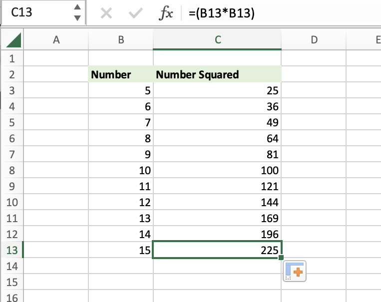
1. In cell C3, enter the following formula:
=(B3*B3)
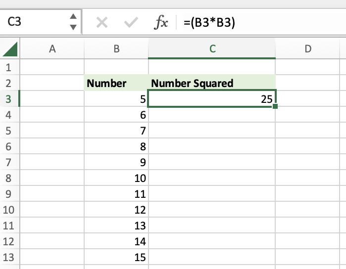
2. Hit enter, and you’ll see the cell populate with the number 25
To fill in the rest of your chart, click the Excel fill handle located in the bottom right corner of cell C3 and drag it through the rest of the cells.
Using the exponent operator
The exponent operator, or the caret symbol (^) in Excel, lets you raise one number to the power of another. Enter this formula in cell C3 to square (raise to the 2nd power) the value in B3:
=(B3^2)
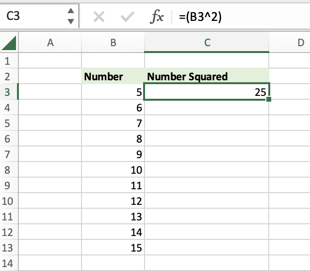
If you’d like to fill in the whole table, use the Excel fill handle to fill the formula down.
Using functions to square a number in Excel
The POWER and PRODUCT functions also make it easy to square a number in Excel!
POWER
The POWER function uses exponents, and you can use it to raise a number to any power.
Formulas that use the POWER function use two arguments: the number that you want to square and the exponent to which you want to raise it.
For example, the following formula will raise 5 to the 2nd power:
=POWER(5,2)
You can also use a cell reference for a function argument, as shown below.
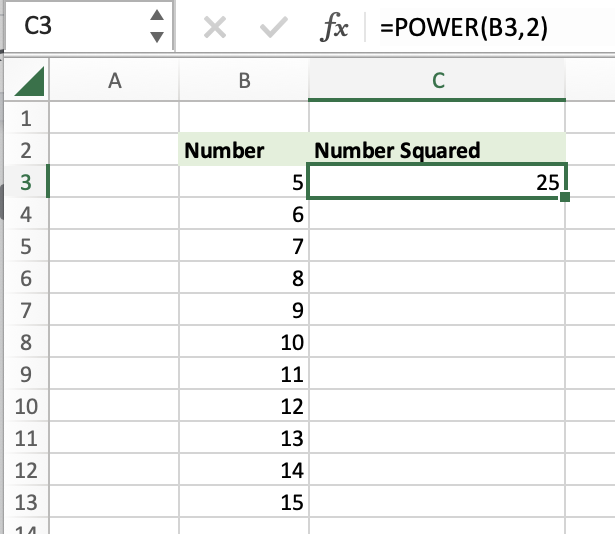
PRODUCT
The PRODUCT function simply multiplies one number by another.
Formulas that contain the PRODUCT function multiply the numbers given as arguments, so to square the number 5, you would use the following formula:
=PRODUCT(5,5)
You can also use cell references as the function arguments, as shown below.
=PRODUCT(B3,B3)
And those are a few different methods for squaring numbers in Excel (and they work in Google Sheets as well). Hopefully this was helpful 🙂
Do you have any other tips for squaring numbers in Excel? Let us know in the comments!