
In Excel for the web, you can view the results of a regression analysis (in statistics, a way to predict and forecast trends), but you can’t create one because the Regression tool isn’t available.
You also won’t be able to use a statistical worksheet function such as LINEST to do a meaningful analysis because it requires you enter it as an array formula, which isn’t supported in Excel for the web.
If you have the Excel desktop application, you can use the Open in Excel button to open your workbook and use either the Analysis ToolPak’s Regression tool or statistical functions to perform a regression analysis there.
Click Open in Excel and perform a regression analysis.
For news about the latest Excel for the web updates, visit the Microsoft Excel blog.
For the full suite of Office applications and services, try or buy it at Office.com.
Need more help?
Want more options?
Explore subscription benefits, browse training courses, learn how to secure your device, and more.
Communities help you ask and answer questions, give feedback, and hear from experts with rich knowledge.
Regression is an Analysis Tool, which we use for analyzing large amounts of data and making forecasts and predictions in Microsoft Excel.
Want to predict the future? No, we are not going to learn astrology. We are into numbers and we will learn regression analysis in Excel today.
To predict future estimates, we will study:
- REGRESSION ANALYSIS USING EXCEL FUNCTIONS (MANUAL REGRESSION FINDING)
- REGRESSION ANALYSIS USING EXCEL’S ANALYSIS TOOLPAK ADD-IN
- REGRESSION CHART IN EXCEL
Let’s do it…
Scenario:
Let’s assume you sell soft drinks. How cool will it be if you can predict:
- How many soft drinks will be sold next year based on previous year’s data?
- Which fields need to be focused?
- And how can you increase your sales by changing your strategy?
It will be profitably awesome. Right?… I know. So let’s get started.
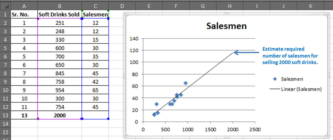
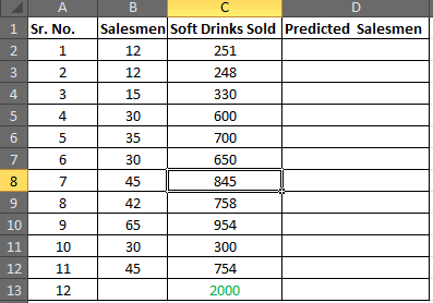
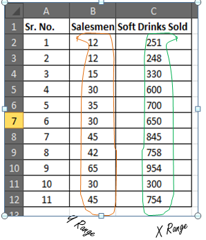
You have 11 records of salesmen and soft drinks sold.
Now based on this data you want to predict the number of salesmen required to achieve 2000 sales of soft drinks.

The regression equation is a tool to make such close estimates. To do so, we need to know Regression first.
REGRESSION ANALYSIS USING EXCEL FUNCTIONS (MANUAL REGRESSION FINDING)
This part will make you understand regression better than just telling excel regression procedure.
Introduction:
Simple Linear Regression:
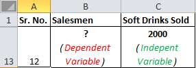
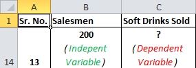
The study of the relationship between two variables is called Simple Linear Regression. Where one variable depends on the other independent variable. The dependent variable is often called by names such as Driven, Response, and Target variable. And the independent variable is often pronounced as a Driving, Predictor or simply Independent variable. These names clearly describe them.

Now let’s compare this with your scenario. You want to know the number of salesmen required to achieve 2000 sales. So here, the dependent variable is the number of salesmen and the independent variable is sold soft drinks.
The independent variable is mostly denoted as x and dependent variable as y.
In our case, soft drinks are sold x and the number of salesmen is y.
If we want to know how many soft drinks will be sold if we appoint 200 salesmen, then the scenario will be vice-versa.
Moving On.
The “Simple” Math of Linear Regression Equation:
Well, it’s not simple. But Excel made it simple to do.
We need to predict the required number of salesmen for all 11 cases to get the 12th closest prediction.
Let’s say:
Soft Drink Sold is x
The number of Salesmen is y
The predicted y (number of salesmen) also called Regression Equation, would be
Now you must be wondering where the stat will you get the slope and intercept. Don’t worry, excel has functions for them. You do not need to learn how to find the slope and intercept it manually.
If you want, I will prepare a separate tutorial for that. Let me know in the comments section. These are some important data analytics tools.
Now let’s step into our calculation:
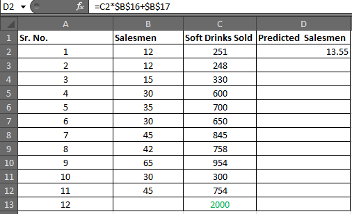
Step1: Prepare this small table
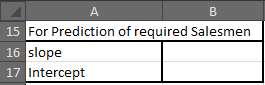
Step 2: Find the slope of the regression line
Excel Function for slopes is
=SLOPE(known_y’s,known_x’s)
Your known_y’s are in range B2:B12 and known_x’s are in range C2:C12

In cell B16, write the formula below
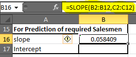
(Note: Slope is also called coefficient of x in the regression equation)
You will get 0.058409. Round up to 2 decimal digits and you will get 0.06.
Step 3: Find the Intercept of Regression Line
Excel function for the intercept is
=INTERCEPT(known_y’s, known_x’s)
We know what our known x’s and y’s
In cell B17, write down this formula

=INTERCEPT(B2:B12, C2:C12)
You will get a value of -1.1118969. Roundup to 2 decimal digits. You will get -1.11.
Our Linear Regression Equation is = x*0.06 + (-1.11). Now we can predict possible y depending on the target x easily.
Step 4: In D2 write the formula below
=C2*$B$16+$B$17 (Regression Equation)
You will get a value of 13.55.
Select D2 to D13 and press CTRL+D to fill down the formula in the range D2:D13
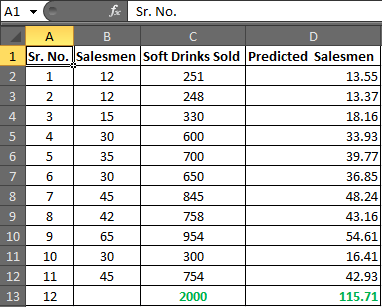
In cell D13 you have your required number of salesmen.
Hence, to achieve the target of 2000 Soft Drink Sales, you need an estimate of 115.71 salesmen or say 116 since it is illegal to cut humans into pieces.
Now using this you can easily conduct What-If analysis in excel. Just change the number of sales and it will show you many salesmen will it take to get that sales target achieved.
Play around it to find out:
How much workforce do you need to increase sales?
How many sales will increase if you increase your salesmen?
Make Your Estimate More Reliable:
Now you know that you need 116 salesmen to get 2000 sales done.
In analytics, nothing is just said and believed. You must give a percentage of reliability on your estimate. It is like giving a certificate of your equation.

Correlation Coefficient Formula:
The next thing you will be asked is how much these two variables are related. In static terms, you need to tell the coefficient of correlation.
Excel function for correlation is
In your case, known_x’s and Know_y’s are array1 and array2 irrespectively.
In B18 enter this formula
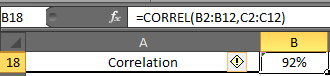
You will have 0.919090. Formate cell B2 into the percentage. Now have 92% of correlation.
Now, what this 92% means. It means, there 92% of chances of sales increase if you increase the number of salesmen and 92% of sales decrease if you decrease the number of salesmen. It is called Positive Correlation Coefficient.
R Squire (R^2) :
R Squire value tells you, by what percentage your regression equation is not a fluke. How much it is accurate by the data provided.
The Excel function for R squire is RSQ.
RSQ(known_y’s, Known_x’s)
In our case, we will get R squire value in cell B19.
In B19 enter this formula

So we have 84% of r Square value. Which is a very good explanation of our regression. It says that 84% of our data is just not by chance. Y (number of salesmen) is very much dependent on X (sales of soft drinks).
There are many other tests we can do on this data to ensure our regression. But manually it will be a complex and lengthy procedure. That is why excel provides Analysis Toolpak. Using this tool we can do this regression analysis in seconds.
REGRESSION IN EXCEL USING EXCEL’S ANALYSIS TOOLPAK ADD-IN
If you already know what regression equations are, and you just want your results quickly then this part is for you. But if you want to understand regression equations easily then scroll up to REGRESSION ANALYSIS USING EXCEL FUNCTIONS (MANUAL REGRESSION FINDING).
Excel provides a whole bunch of tools for analysis in its Analysis Toolpak. By default, it is not available in the Data tab. You need to add it. So let’s add it first.
Adding Analysis Toolpak to Excel 2016
If you don’t know where is data analysis in excel follow these steps
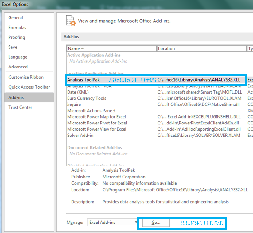
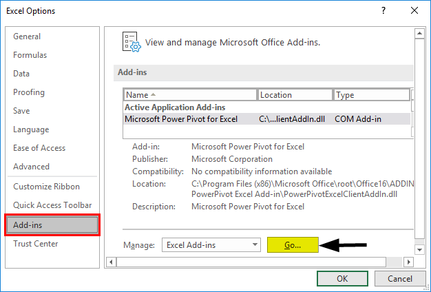
Step 1: Go to Excel Options: File? Options? Add-Ins
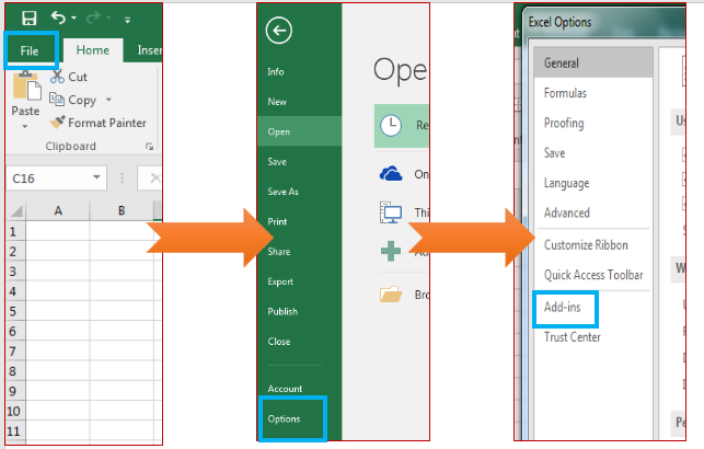
Step 2: Click on Add-Ins. You will see a list of available add-Ins.
Select Analysis ToolPak and at the bottom of the window, find manage. In manage select Excel Add-Ins and Click on GO.
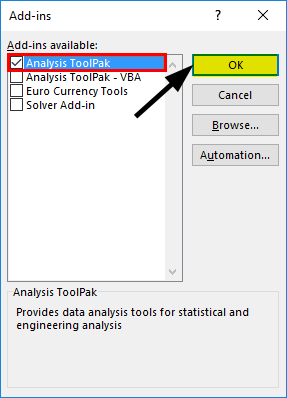
Add-ins window will open. Here, select Analysis ToolPak. Then click the ok button.
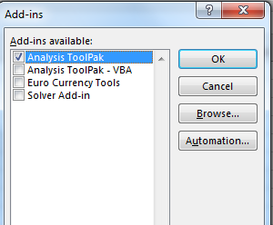
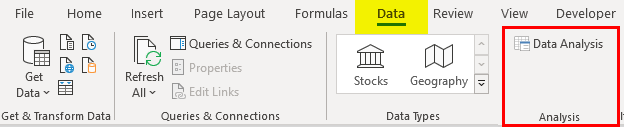
Now you can access all functions of data analysis ToolPak from Data Tab.
Using Analysis ToolPak for Regression
Step 1: Go to the Data tab, Locate Data Analysis. Then click on it.

A dialogue box will pop up.
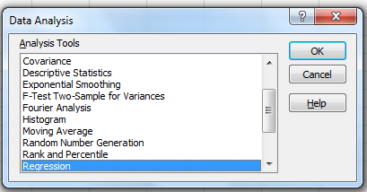
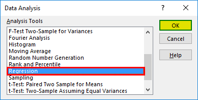
Step 2: Find ‘Regression’ in Analysis Tools list and hit the OK button.
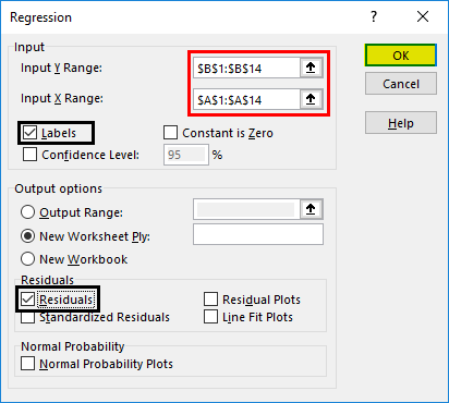
The regression input window will pop up. You will see a number of available input options. But for now, we will just concentrate on Y Range and X Range, leaving everything else to default.

Step 4: Provide Inputs:
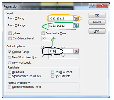
No. of Salesmen is Y
Sales of soft drinks are X
Hence
- Y Range= B2:B11
And
- X Range = C2:C11
For the output range, I have selected E4 on the same sheet. You may select a new worksheet to get results on a new worksheet in the same workbook or a complete new workbook. When you are done with your inputs, hit the OK button.
Results:
You will be served with a variety of information from your data. Don’t get overwhelmed. You don’t need to consume all the dishes.
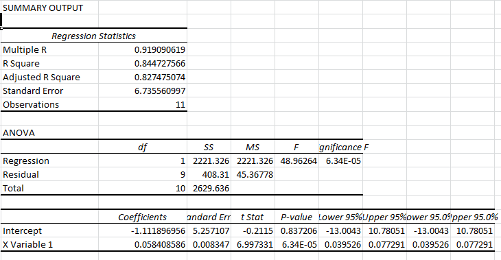
We will only deal with those results which will help us to estimate the required number of salesmen
Step 5: We know the regression equation for estimation of y, that is
x*Slope+Intercept
We just need to locate Slope and Intercept in results.
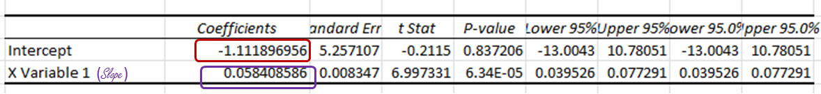
And here they are.
The intercept Coefficient is clearly mentioned.
The slope is written as ‘X Variable 1’, some times also mentioned as the coefficient of X. Round up them and we will get -1.11 as Intercept and 0.06 as Slope.
Step 6: From results, we can drive the Regression equation. And that would be
=x*(0.06) + (-1.11)
Prepare this table in excel.

For now, x is 2000, which is in cell E2.
In Cell F2 enter this formula
=E2*F21+F20
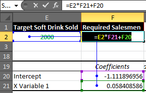
You will get a result of 115.7052757.

Rounding it up will give us 116 of Required Salesmen.
So we have learned how to form the regression equation manually and using Analysis ToolPak. How can you use this equation to estimate future stats?
Now let’s understand the regression output given by Analysis Toolpak.
Understanding the Regression Output:
There is no benefit, if you do regression analysis using analysis tool pack in excel and can’t interpret its meaning.
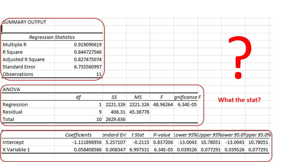
Summary Section:
As the name suggests, it is a summary of the data.

-
- Multiple R: It tells how fit the regression equation is to the data. It is also called the correlation coefficient.
In our case, it is 0.919090619 or 0.92 (roundup). This means that there is a 92% chance of an increase in sales if we increase our salesmen count.
-
- R Square: It tells the reliability of found regression. It tells us how many observations are part of our line of regression. In our case, it is 0.844727566 or 0.85. It means that our regression is fit by 85%.
- Adjusted R Square: Theadjusted square is just a more testified version of R square. Mainly useful in Multiple Regression Analysis.
- Standard Error: While R. Squire tells you how many data points fall near the regression line, the standard error tells you how far a data point can go from the regression line.
In our case, it is 6.74.
- Observation: This is simply the number of observations, which is 11 in our example.
Anova Section:
This section is hardly used in linear regression.
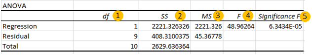
- df. It is a degree of freedom. It is used when calculating regression manually.
- SS. Sum of squares. It is just a sum of squares of variances. Used to find R squire values.
- MS. This means squared value.
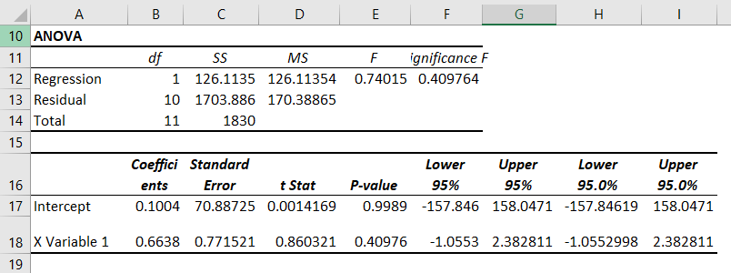
- And 5. F and Significance of F. If the significance of F (p-value of the slope) is less than the F test than you can discard the null hypothesis and prove your hypothesis. In simple language, you can conclude that there is some effect of x on y when changed.
In our case, F is 48.96264 and Significance of F is 0.000063. It means our regression fits the data.
Regression Section:
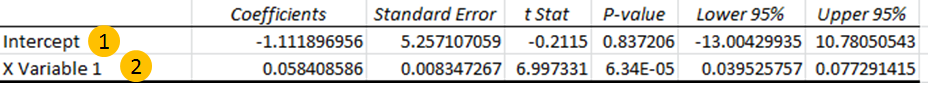
In this section, we have the two most important values for our regression equation.
- Intercept: We have an intercept here that tells where x-intercepts on Y. This is an important part of the regression equation. It is -1.11 in our case.
- X variable 1 (Slope). Also called the coefficient of x. It defines the tangent of the regression line.
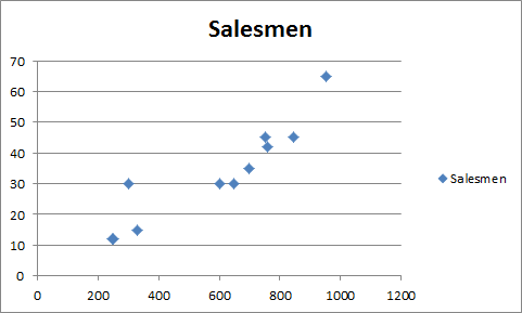
REGRESSION CHART IN EXCEL
In excel, it is easy to plot a regression chart. Just follow these steps. To add Regression Chart in Excel 2016, 2013, and 2010 follow these simple steps.
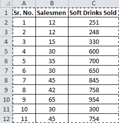
Step 1. Have your known x’s in the first column and know y’s in the second.
In our case, we know Known_ x’s are Soft Drinks Sold. And known_y’s are Salesmen.

Step 2. Select your known x’s and y’s range.

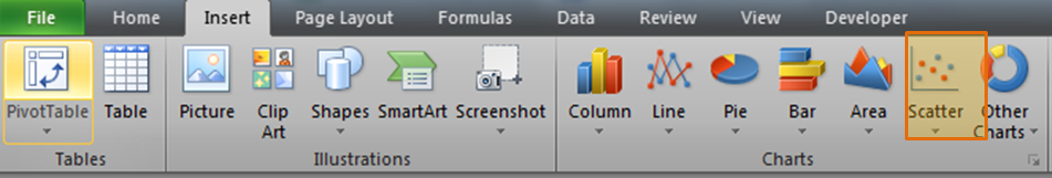
Step 3: Go to the Insert tab and click on the scatter chart.
You will have a chart that looks like this.
Step 4. Add the trend line: Goto layout and locate the trendline option in the analysis section.
Under the Trendline option, click on Linear Trendline.
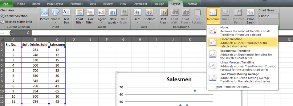
You will have your graph looking like this.
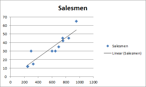
This is your regression graph.
Now if you add the data below and extend the selected data. You will see a change in your graph.
For our example, we added 2000 to the Soft Drink Sold and left the Salesmen blank. And when we extend the range of the graph, this is what we will have.
It will give the required number of salesmen for doing 2000 sales of soft drinks in graphical form. Which is slightly below 120 in the graph. And from our regression equation, we know it is 116.

In this article, I tried to cover everything under Excel Regression Analysis. I explained regression in excel 2016. Regression in excel 2010 and excel 2013 is same as in excel 2016.
For any further query on this topic, use the comments section. Ask a question, give an opinion or just mention my grammatical mistakes. Everything is welcome. Just don’t hesitate to use the comment section.
Related Data:
How to Use STDEV Function in Excel
How To Calculate MODE function in Excel
How To Calculate Mean function in Excel
How to Create Standard Deviation Graph
Descriptive Statistics in Microsoft Excel 2016
How to Use Excel NORMDIST Function
How to use the Pareto Chart and Analysis
Popular Articles:
50 Excel Shortcut to Increase Your Productivity
How to use the VLOOKUP Function in Excel
How to use the COUNTIF function in Excel 2016
How to use the SUMIF Function in Excel
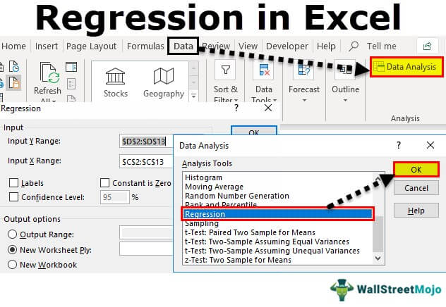
Regression is done to define relationships between two or more variables in a data set. In statistics, regression is done by some complex formulas. But, Excel has provided us with tools for regression analysis. So, in the Excel Analysis ToolPak, click “Data Analysis” and “Regression” to conduct regression analysis in Excel.
Table of contents
- What is Regression Analysis in Excel?
- Explained
- Examples
- How to Run Regression Analysis Tool in Excel?
- How to Use Regression Analysis Tool in Excel?
- Steps to Create Regression Chart in Excel
- Things to Remember
- Recommended Articles
Explained
The Regression analysis tool performs linear regression in excelLinear Regression is a statistical excel tool that is used as a predictive analysis model to examine the relationship between two sets of data. Using this analysis, we can estimate the relationship between dependent and independent variables.read more examination using the “minimum squares” technique to fit a line through many observations. You can examine how an individual dependent variable is influenced by the estimations of at least one independent variable. For instance, you can investigate how such factors influence a sportsman’s performance as age, height, and weight. You can distribute shares in the execution measure to every one of these three components, given a lot of execution information, and then utilize the outcomes to foresee the execution of another person.
The Excel regression analysis tool helps you see how the dependent variable changes when one of the independent variables fluctuates and permits you to numerically figure out which of those variables truly has an effect.
You are free to use this image on your website, templates, etc, Please provide us with an attribution linkArticle Link to be Hyperlinked
For eg:
Source: Regression Analysis in Excel (wallstreetmojo.com)
Examples
- Sales of shampoo are dependent upon the advertisement. If $1 million increases advertising expenditure, sales will be expected to increase by $23 million. If there were no advertising, we would expect sales without any increment.
- House sales (selling price, number of bedrooms, location, size, design) predict the selling price of future sales in the same area.
- Soft drink sales massively increase in summer when the weather is too hot. People purchase more and more soft drinks to keep them cool. The higher the temperature, the higher the sales and vice versa.
- In March, exam season started, and sales increased due to students purchasing exam pads. Exam pads sale depends upon the examination season.
How to Run Regression Analysis Tool in Excel?
- We must enable the Analysis ToolPak Add-in.
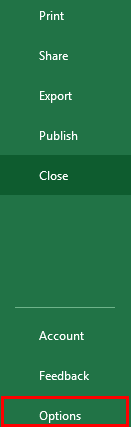
- In Excel, click on the “File” on the extreme left-hand side, go and click on the “Options” at the end.

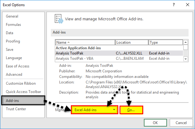
- On clicking on “Options,” select “Add-ins” on the left side. Excel Add-ins are chosen in the “View and manage Microsoft Add-ins” and “Manage” boxes. Then, click “Go.”

- In the Add-in dialog box, click on Analysis Toolpak, and click OK:

It will add the “Data Analysis” tools on the right-hand side to the Excel ribbon’s “Data” tab.


How to Use Regression Analysis Tool in Excel?
We must use the data for regression analysis in Excel.
You can download this Regression Excel Template here – Regression Excel Template
Once Analysis ToolpakExcel’s data analysis toolpak can be used by users to perform data analysis and other important calculations. It can be manually enabled from the addins section of the files tab by clicking on manage addins, and then checking analysis toolpak.read more is added and enabled in the Excel workbook, follow the steps mentioned below to practice the analysis of regression in Excel:
- Step 1: On the Data tab in the Excel ribbonThe ribbon is an element of the UI (User Interface) which is seen as a strip that consists of buttons or tabs; it is available at the top of the excel sheet. This option was first introduced in the Microsoft Excel 2007.read more, click the Data Analysis

- Step 2: Click on the “Regression” and click “OK” to enable the function.

- Step 3: On clicking the “Regression“ dialog box, we must arrange the accompanying settings:
- For the dependent variable, select the “Input Y Range,” which denotes the dependent data. Here, in the below-given screenshot, we have selected the range from $D$2:$D$13.

- Select the “Input X Range,” which denotes the independent data for the independent variable. Here, in the below-given screenshot, we have selected the range from $C$2:$C$13.

- Step 4: Click “OK” and analyze the data accordingly.

When you run the regression analysis in Excel, the following output will come:


You can also make a scatter plot in excelScatter plot in excel is a two dimensional type of chart to represent data, it has various names such XY chart or Scatter diagram in excel, in this chart we have two sets of data on X and Y axis who are co-related to each other, this chart is mostly used in co-relation studies and regression studies of data.read more of these residuals.
Steps to Create Regression Chart in Excel
- Step 1: Select the data as given in the below screenshot.

- Step 2: Tap on the “Inset” tab. In the “Charts” gathering, tap the “Scatter” diagram or some other as a required symbol. Select the chart which suits the information.

- Step 3: We can modify the chart when required and fill in the hues and lines of your decision. For instance, we can pick alternate shading and utilize a strong line of a dashed line. We can customize the graph as we want to customize it.

Things to Remember
- We must always check the dependent and independent values. Otherwise, the analysis will be wrong.
- If you test a huge number of data and thoroughly rank them based on their validation period statisticsStatistics is the science behind identifying, collecting, organizing and summarizing, analyzing, interpreting, and finally, presenting such data, either qualitative or quantitative, which helps make better and effective decisions with relevance.read more.
- Choose the data carefully to avoid any kind of error in excel analysis.
- We can optionally check any of the boxes at the bottom of the screen, although none of these is necessary to obtain the line best-fit formula.
- Start practicing with small data to understand the better analysis and run the regression analysis tool in Excel easily.
Recommended Articles
This article is a step-by-step guide to Regression Analysis in Excel. Here we discuss how to run regression in Excel, its interpretation, and use this tool along with Excel examples and downloadable Excel templates. You may also look at these useful functions in Excel: –
- Examples of Normal Distribution Graph in Excel
- Regression vs. ANOVABoth the Regression and ANOVA are the statistical models which are used in order to predict the continuous outcome but in case of the regression, continuous outcome is predicted on basis of the one or more than one continuous predictor variables whereas in case of ANOVA continuous outcome is predicted on basis of the one or more than one categorical predictor variables.read more
- Excel Exponential Smoothing
- Exponential Function ExcelExponential Excel function(EXP) is an inbuilt function in excel used to calculate the exponent raised to the power of any number you provide. In this function the exponent is constant and is also known as the base of the natural algorithm.read more
Reader Interactions
We can chart a regression in Excel by highlighting the data and charting it as a scatter plot. To add a regression line, choose “Layout” from the “Chart Tools” menu. In the dialog box, select “Trendline” and then “Linear Trendline”. To add the R2 value, select “More Trendline Options” from the “Trendline menu.
Contents
- 1 How do you create a linear regression in Excel?
- 2 How do you do a linear regression on a spreadsheet?
- 3 How do you do linear regression step by step?
- 4 How do you find R2 on Excel?
- 5 How do I add data analysis to Excel?
- 6 How do you do a regression in Excel with multiple variables?
- 7 How do you write a simple linear regression equation?
- 8 How do you find b0 and b1 in linear regression?
- 9 How do you calculate linear regression by hand?
- 10 What is a regression equation example?
- 11 What does R 2 mean Excel?
- 12 What is R2 in Excel Trendline?
- 13 Where is data analysis Excel 2021?
- 14 Is Excel good for data analysis?
- 15 Is Excel a data analysis tool?
- 16 What is the formula for multiple linear regression?
- 17 What is linear regression for dummies?
- 18 How do you find b0 and b1 in Excel?
- 19 How do you do regression analysis on Excel?
- 20 How do you write a null hypothesis for a linear regression?
How do you create a linear regression in Excel?
Add the regression line by choosing the “Layout” tab in the “Chart Tools” menu. Then select “Trendline” and choose the “Linear Trendline” option, and the line will appear as shown above.
How do you do a linear regression on a spreadsheet?
To get a linear regression of any data, follow the steps below;
- Step 1: Prepare the data.
- Step 2: Highlight the data.
- Step 3: Get the scatter graph.
- Step 4: Choose scatter plot.
- Step 5: Get the trendline.
- Step 6: Changing the label.
How do you do linear regression step by step?
- Step 1: Load the data into R. Follow these four steps for each dataset:
- Step 2: Make sure your data meet the assumptions.
- Step 3: Perform the linear regression analysis.
- Step 4: Check for homoscedasticity.
- Step 5: Visualize the results with a graph.
- Step 6: Report your results.
How do you find R2 on Excel?
Double-click on the trendline, choose the Options tab in the Format Trendlines dialogue box, and check the Display r-squared value on chart box.
How do I add data analysis to Excel?
Click the File tab, click Options, and then click the Add-Ins category. In the Manage box, select Excel Add-ins and then click Go. In the Add-Ins box, check the Analysis ToolPak check box, and then click OK.
How do you do a regression in Excel with multiple variables?
In Excel you go to Data tab, then click Data analysis, then scroll down and highlight Regression. In regression panel, you input a range of cells with Y data, with X data (multiple regressors), check the box with output range or new worksheet, and check all the plots that you need.
How do you write a simple linear regression equation?
The Linear Regression Equation
The equation has the form Y= a + bX, where Y is the dependent variable (that’s the variable that goes on the Y axis), X is the independent variable (i.e. it is plotted on the X axis), b is the slope of the line and a is the y-intercept.
How do you find b0 and b1 in linear regression?
The mathematical formula of the linear regression can be written as y = b0 + b1*x + e , where: b0 and b1 are known as the regression beta coefficients or parameters: b0 is the intercept of the regression line; that is the predicted value when x = 0 . b1 is the slope of the regression line.
How do you calculate linear regression by hand?
Linear Regression by Hand and in Excel
- Calculate average of your X variable.
- Calculate the difference between each X and the average X.
- Square the differences and add it all up.
- Calculate average of your Y variable.
- Multiply the differences (of X and Y from their respective averages) and add them all together.
What is a regression equation example?
A regression equation is used in stats to find out what relationship, if any, exists between sets of data. For example, if you measure a child’s height every year you might find that they grow about 3 inches a year. That trend (growing three inches a year) can be modeled with a regression equation.
What does R 2 mean Excel?
R squared is an indicator of how well our data fits the model of regression. Also referred to as R-squared, R2, R^2, R2, it is the square of the correlation coefficient r. The correlation coefficient is given by the formula: Figure 1.
What is R2 in Excel Trendline?
When adding a trendline in Excel, you have 6 different options to choose from.Trendline equation is a formula that finds a line that best fits the data points. R-squared value measures the trendline reliability – the nearer R2 is to 1, the better the trendline fits the data.
Where is data analysis Excel 2021?
Q. Where is the data analysis button in Excel?
- Click the File tab, click Options, and then click the Add-Ins category.
- In the Manage box, select Excel Add-ins and then click Go.
- In the Add-Ins available box, select the Analysis ToolPak check box, and then click OK.
Is Excel good for data analysis?
Excel is a great tool for analyzing data. It’s especially handy for making data analysis available to the average person at your organization.
Is Excel a data analysis tool?
The Analysis ToolPak is an Excel add-in program that provides data analysis tools for financial, statistical and engineering data analysis.
What is the formula for multiple linear regression?
Since the observed values for y vary about their means y, the multiple regression model includes a term for this variation. In words, the model is expressed as DATA = FIT + RESIDUAL, where the “FIT” term represents the expression 0 + 1x1 + 2x2 +xp.
What is linear regression for dummies?
Statistical researchers often use a linear relationship to predict the (average) numerical value of Y for a given value of X using a straight line (called the regression line). If you know the slope and the y-intercept of that regression line, then you can plug in a value for X and predict the average value for Y.
How do you find b0 and b1 in Excel?
Use [email protected] =LINEST(ArrayY, ArrayXs) to get b0, b1 and b2 simultaneously.
How do you do regression analysis on Excel?
Run regression analysis
- On the Data tab, in the Analysis group, click the Data Analysis button.
- Select Regression and click OK.
- In the Regression dialog box, configure the following settings: Select the Input Y Range, which is your dependent variable.
- Click OK and observe the regression analysis output created by Excel.
How do you write a null hypothesis for a linear regression?
For simple linear regression, the chief null hypothesis is H0 : β1 = 0, and the corresponding alternative hypothesis is H1 : β1 = 0. If this null hypothesis is true, then, from E(Y ) = β0 + β1x we can see that the population mean of Y is β0 for every x value, which tells us that x has no effect on Y .
R Square | Significance F and P-Values | Coefficients | Residuals
This example teaches you how to run a linear regression analysis in Excel and how to interpret the Summary Output.
Below you can find our data. The big question is: is there a relation between Quantity Sold (Output) and Price and Advertising (Input). In other words: can we predict Quantity Sold if we know Price and Advertising?

1. On the Data tab, in the Analysis group, click Data Analysis.

Note: can’t find the Data Analysis button? Click here to load the Analysis ToolPak add-in.
2. Select Regression and click OK.

3. Select the Y Range (A1:A8). This is the predictor variable (also called dependent variable).
4. Select the X Range(B1:C8). These are the explanatory variables (also called independent variables). These columns must be adjacent to each other.
5. Check Labels.
6. Click in the Output Range box and select cell A11.
7. Check Residuals.
8. Click OK.

Excel produces the following Summary Output (rounded to 3 decimal places).
R Square
R Square equals 0.962, which is a very good fit. 96% of the variation in Quantity Sold is explained by the independent variables Price and Advertising. The closer to 1, the better the regression line (read on) fits the data.

Significance F and P-values
To check if your results are reliable (statistically significant), look at Significance F (0.001). If this value is less than 0.05, you’re OK. If Significance F is greater than 0.05, it’s probably better to stop using this set of independent variables. Delete a variable with a high P-value (greater than 0.05) and rerun the regression until Significance F drops below 0.05.
Most or all P-values should be below below 0.05. In our example this is the case. (0.000, 0.001 and 0.005).

Coefficients
The regression line is: y = Quantity Sold = 8536.214 -835.722 * Price + 0.592 * Advertising. In other words, for each unit increase in price, Quantity Sold decreases with 835.722 units. For each unit increase in Advertising, Quantity Sold increases with 0.592 units. This is valuable information.
You can also use these coefficients to do a forecast. For example, if price equals $4 and Advertising equals $3000, you might be able to achieve a Quantity Sold of 8536.214 -835.722 * 4 + 0.592 * 3000 = 6970.
Residuals
The residuals show you how far away the actual data points are fom the predicted data points (using the equation). For example, the first data point equals 8500. Using the equation, the predicted data point equals 8536.214 -835.722 * 2 + 0.592 * 2800 = 8523.009, giving a residual of 8500 — 8523.009 = -23.009.

You can also create a scatter plot of these residuals.

How to do Linear Regression in Excel: Full Guide (2023)
Linear regression is an easy way of evaluating the relationship between two variables.
Previously, performing linear regression in Excel was nothing less than a complex task. But with advanced Excel data analysis tools, it is now only a matter of a few clicks.
The guide below will not only teach you how to perform linear regression in Excel but also how you may analyze a linear regression graph in Excel.
So, without further ado, let’s dive right in 👇
Download our free sample workbook here as you continue reading.
Linear regression equation
Simple linear regression draws the relationship between a dependent and an independent variable.
👉 The dependent variable is the variable that needs to be predicted (or whose value is to be found).
👉 The independent variable explains (or causes) the change in the dependent variable.
Simply put, the dependent variable depends upon the independent variable. And as the independent variable changes, the dependent variable changes too.
Mathematically, the linear relationship between these two variables is explained as follows:
Y= a + bx
Where,
Y = dependent variable
a = regression intercept term
b = regression slope coefficient
x = independent variable
“a” and “b” are also called regression coefficients. And Excel returns the predicted values of these regression coefficients too.
How to do linear regression through a graph
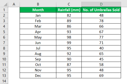
Imagine a company that sells sweaters in a cold region. And the sale of sweaters is directly linked to the temperatures in that region.
The colder it is (low temperatures 🥶), the higher the sales of sweaters 🧣 go. This means sales (the dependent variable) depend upon the temperature (the independent variable).
Now, to predict the company’s sales for the future, you must analyze the sales trend in the past. This can be done by drawing a trendline.
Drawing this trendline between a dependent variable Y (the sales) and an independent variable X (the temperature) is called running linear regression.
So let’s do it!

The image above contains the historical data for both variables (temperatures and sales) for a few months.
To explain the relationship between these variables, we need to make a scatter plot.
To plot the above data in a scatter plot in Excel:
- Select the data.
- Go to the Insert Tab > Charts Group

- Click on the scatterplot part icon.
- Choose a scatter plot type from the drop-down menu.

Excel plots the data in a scatter plot.

Note that each dot in the scatter plot above is formed at the intersection of Variable X and Y.
For example, the first dot is plotted at the point where Y = 625 and X = 2.
Next, we must draw a trend line out of this scatter plot. To do so:
- Click anywhere on the chart to select it.
- Click on the “+” icon on the top right of the chart.

- Hover your cursor over the option “Trendline”📈
A drop-down menu appears.

- Select More Options. This will take you to the Format Trendline Pane.
- Choose the linear trendline option to draw a trendline between the scatter points.

And there you go! Excel draws a linear trendline on the scatterplot.

The above image shows a downward regression line which represents a negative trend. But why is that?
To understand that, you must know how to analyze the results of a linear regression graph. And don’t worry – it’s only a section ahead.
Adding the equation and R-squared
We also want Excel to show the equation and R-squared for this graph. For that:
- Scroll down the Task pane.
- Check the option for “Equation” and “R-squared” on the graph.

And Excel will display the following regression statistics on the graph:
Equation: y= -19.622x + 612.77
R-squared= 0.7456

What are these? And what do they tell? We will discuss this shortly.
Pro Tip!
How to quickly interpret the relationship between two variables? By checking the sign of the x variable 💡
A positive sign means a positive relationship. And a negative sign means a negative relationship between the two variables.
Since our equation shows a “-19.622x”, the relation between our variables is negative.
Formatting the trendline
Do you also find the trendline a little overshadowed? Not to worry – You can always format it in Excel.
For example, to change the color of the trendline:
- Select the trendline and right-click on it to launch the context menu.
- Go to Format Trendline.
- Under the Format Trendline pane, select “Fill & Line”.
- To change the color of the trendline, choose a color as shown below.

Guess we will go with red for now 🚩 What do you think about it?

Trendline Style
Not only the color, but you can also change the style of the trendline.
Say, we want to change our dotted trendline to a solid one. To do so:
- Select the trendline and right-click on it to launch the context menu.
- Click on Format Trendline to launch the Format Trendline Pane.
- Go to “Dash type” from the fill & line menu.
- Select a solid line type.

This will change the style of the trendline from a dotted line to a perfectly solid line.

Chart Title
To enhance the readability of the graph, you may add graph titles and axes titles to it as follows:
- Select the graph.
- Go to Chart Elements > Chart Title > above chart.

- Type in a Graph/Chart title as desired.

Axis titles
How about adding the Axis titles too?
To add a vertical title (for the Y-axis) to your chart:
- Click Chart Elements > Axis Titles > Primary Vertical.

- Type in a suitable title for the subject axis.
We have set the title for the Y-axis to “Sale of Sweaters”.

To add a horizontal Axis Title (for the X-axis):
- Go to Chart elements > Axis Titles > Primary Horizontal.

- Type in a suitable title for the subject axis.
We have set the title for the X-axis to “Avg. Temperature”

And that’s it. We’ve successfully run linear regression in Excel 🥳
How to analyze the linear regression graph
Good job with running linear regression in Excel.
Now is the time that we analyze the linear regression trendline formed above.
A linear trendline in Excel can take the following three shapes:
Positive trendline (upward facing)
If your trendline is upward facing (it elevates as it goes from left to right), it denotes a positive trend.
This means that there exists a positive relationship between both variables. An increase in the independent variable causes the dependent variable to increase.
This is how your graph will look with a positive trendline to it.

Negative trendline (downward sloping)
If your trendline is downward sloping (it slopes down as it goes from left to right), it denotes a negative trend.
A negative trendline means a negative relationship between both variables.
When there is a negative relationship between two variables, an increase in the independent variable causes the dependent variable to decrease.
This is how your graph will look with a negative trendline to it.

Jog down your memory lane to remember the trendline type in our example above. It was also a downward-sloping (negative) trendline.
That’s because there exists a negative relationship between sales and temperature. As the temperature falls, sales increase.
No trend
The two variables can also be independent of each other. In this case, movement in both variables is random with no relation to each other.
As there exists no relationship between them (neither positive nor negative), there is no particular slope for the trendline between them (neither upward facing nor downward sloping).
Such a trendline might look like this.

The trendline above is not exactly horizontal but very close to that. This is because there is no relation between the variables.
The slope of the graph
What if we want to know the percentage of change in Y caused by a change in X?
For example, for every 1% decrease in temperature, sales increase by what percentage?
The slope of the graph is an answer to this. Remember the linear regression equation?
Y = a + bx
In the above equation, the slope is represented by “b”. And the linear regression equation for our example turned out as follows:
Y= 612.77 – 19.622x
Here, the value for b is -19.622 and so is our slope. This means that a 1% change in the X variable (the temperature) causes a -19.622% change in the Y variable (the sales).
Also, as the sign with the value for b is a minus sign, this means that a 1% decrease in Variable X (temperature) causes a 19.622% increase in Variable Y (Sales).

Pro Tip!
An easy way to remember the slope is to remember Rise over Run. Rise means vertical axis. Run means horizontal axis. So the slope defines the change in variable Y caused by a change in variable X.
R-Squared
Another important output of our scatterplot is the R-squared value 👀
It tells us how much variation of the dependent variable comes from the change in the independent variable.

The R-squared for our example is 0.7456.
This tells that only 74.56% variation of Variable Y can be explained by Variable X.
Another statistical measure relevant to the linear regression model is the p value. However, it is totally opposite to the concept of R-squared.
That’s it – Now what?
The above guide explains how to perform a linear regression analysis in Excel. And then, how to analyze the linear regression trendline and other relevant statistics.
👉 In addition to that, it also explains how you may format a trendline in Excel in different ways.
Performing linear regression in Excel through a scatter plot is super smart. But this is only one feature of Excel.
And there are many more smart functions in Excel. Like the VLOOKUP, SUMF, and IF functions.
Want to learn them already? Enroll in my 30-minute free email course that teaches you these and many more functions of Excel.
Other resources
Linear regression can be challenging to understand. But once you get a hold of it, you can run it for any possible dataset with sheer ease.
In addition to linear regression, Excel offers other forecasting functions too. Like the data analysis tools in Excel and the Excel FORECAST function.
Kasper Langmann2023-02-23T14:55:48+00:00
Page load link
Простая линейная регрессия — это метод, который мы можем использовать для понимания взаимосвязи между объясняющей переменной x и переменной отклика y.
В этом руководстве объясняется, как выполнить простую линейную регрессию в Excel.
Пример: простая линейная регрессия в Excel
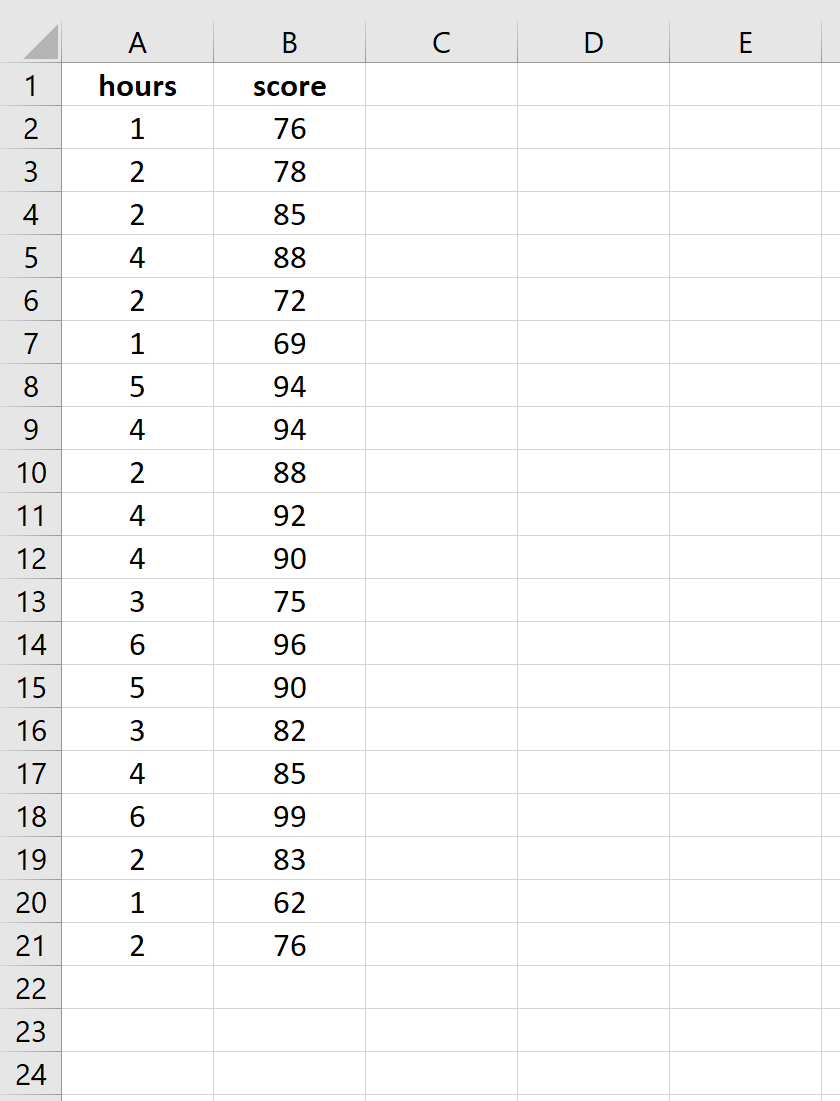
Предположим, нас интересует взаимосвязь между количеством часов, которое студент тратит на подготовку к экзамену, и полученной им экзаменационной оценкой.
Чтобы исследовать эту взаимосвязь, мы можем выполнить простую линейную регрессию, используя часы обучения в качестве независимой переменной и экзаменационный балл в качестве переменной ответа.
Выполните следующие шаги в Excel, чтобы провести простую линейную регрессию.
Шаг 1: Введите данные.
Введите следующие данные о количестве часов обучения и экзаменационном балле, полученном для 20 студентов:
Шаг 2: Визуализируйте данные.
Прежде чем мы выполним простую линейную регрессию, полезно создать диаграмму рассеяния данных, чтобы убедиться, что действительно существует линейная зависимость между отработанными часами и экзаменационным баллом.
Выделите данные в столбцах A и B. В верхней ленте Excel перейдите на вкладку « Вставка ». В группе « Диаграммы » нажмите « Вставить разброс» (X, Y) и выберите первый вариант под названием « Разброс ». Это автоматически создаст следующую диаграмму рассеяния:
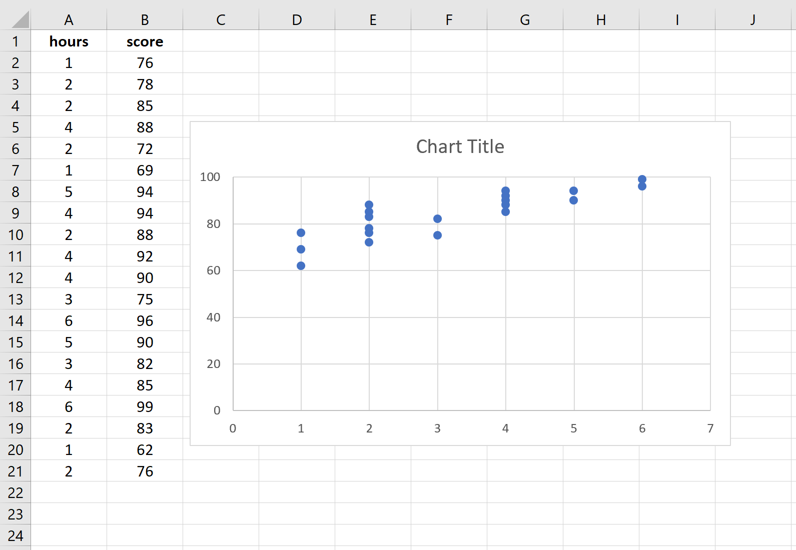
Количество часов обучения показано на оси x, а баллы за экзамены показаны на оси y. Мы видим, что между двумя переменными существует линейная зависимость: большее количество часов обучения связано с более высокими баллами на экзаменах.
Чтобы количественно оценить взаимосвязь между этими двумя переменными, мы можем выполнить простую линейную регрессию.
Шаг 3: Выполните простую линейную регрессию.
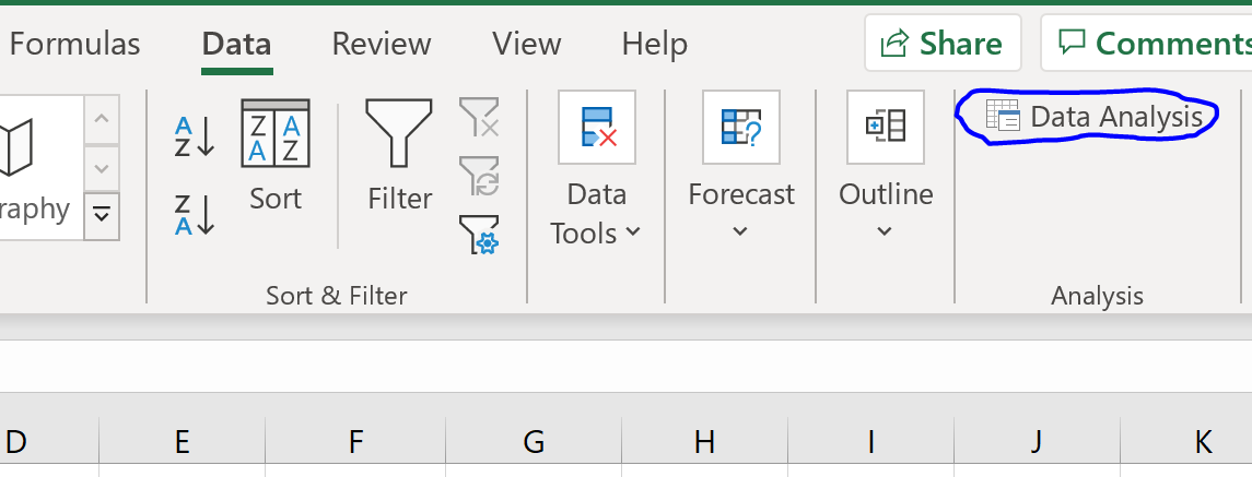
В верхней ленте Excel перейдите на вкладку « Данные » и нажмите « Анализ данных».Если вы не видите эту опцию, вам необходимо сначала установить бесплатный пакет инструментов анализа .
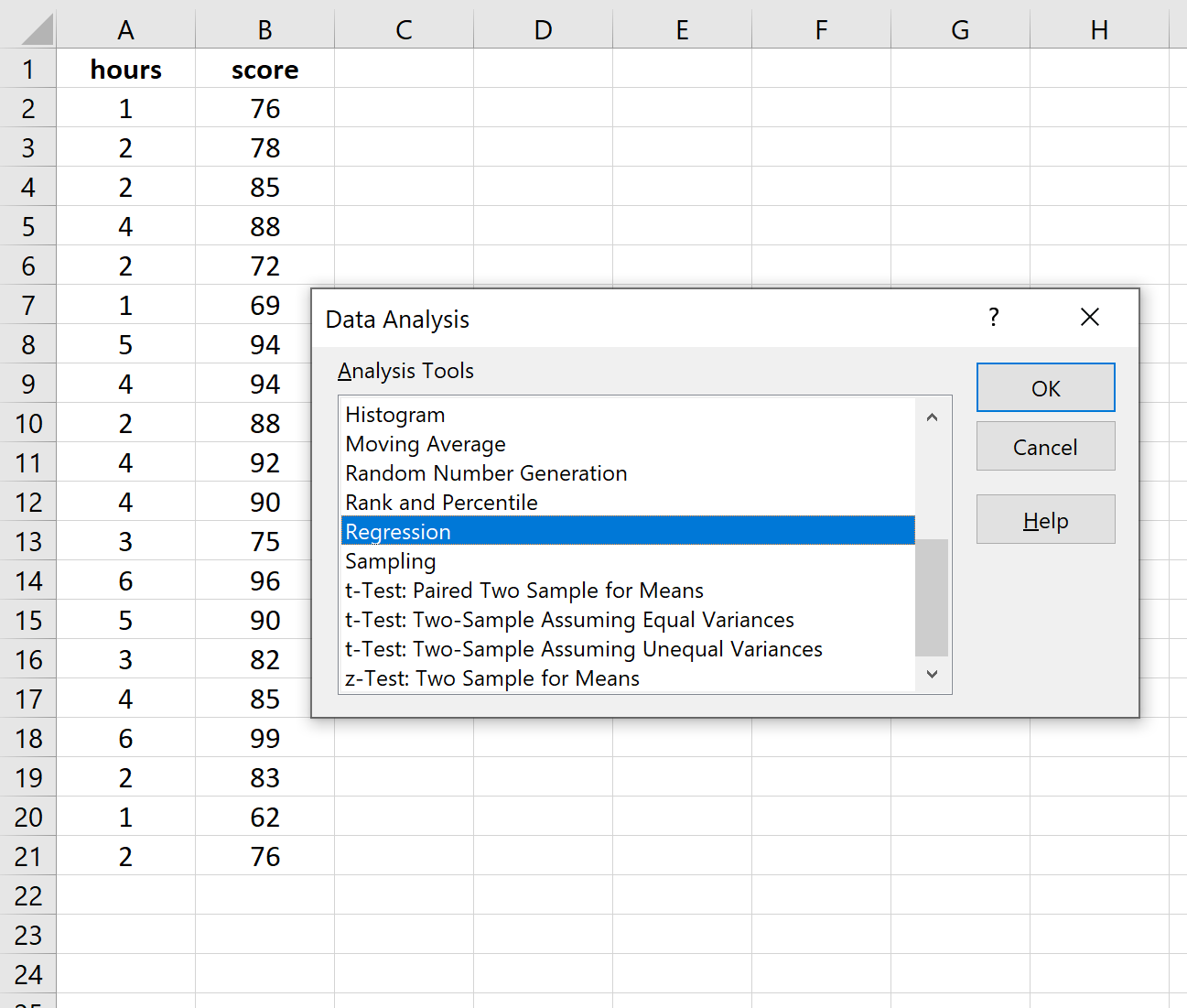
Как только вы нажмете « Анализ данных», появится новое окно. Выберите «Регрессия» и нажмите «ОК».
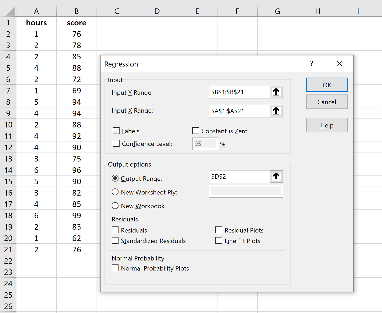
Для Input Y Range заполните массив значений для переменной ответа. Для Input X Range заполните массив значений для независимой переменной.
Установите флажок рядом с Метки , чтобы Excel знал, что мы включили имена переменных во входные диапазоны.
В поле Выходной диапазон выберите ячейку, в которой должны отображаться выходные данные регрессии.
Затем нажмите ОК .
Автоматически появится следующий вывод:
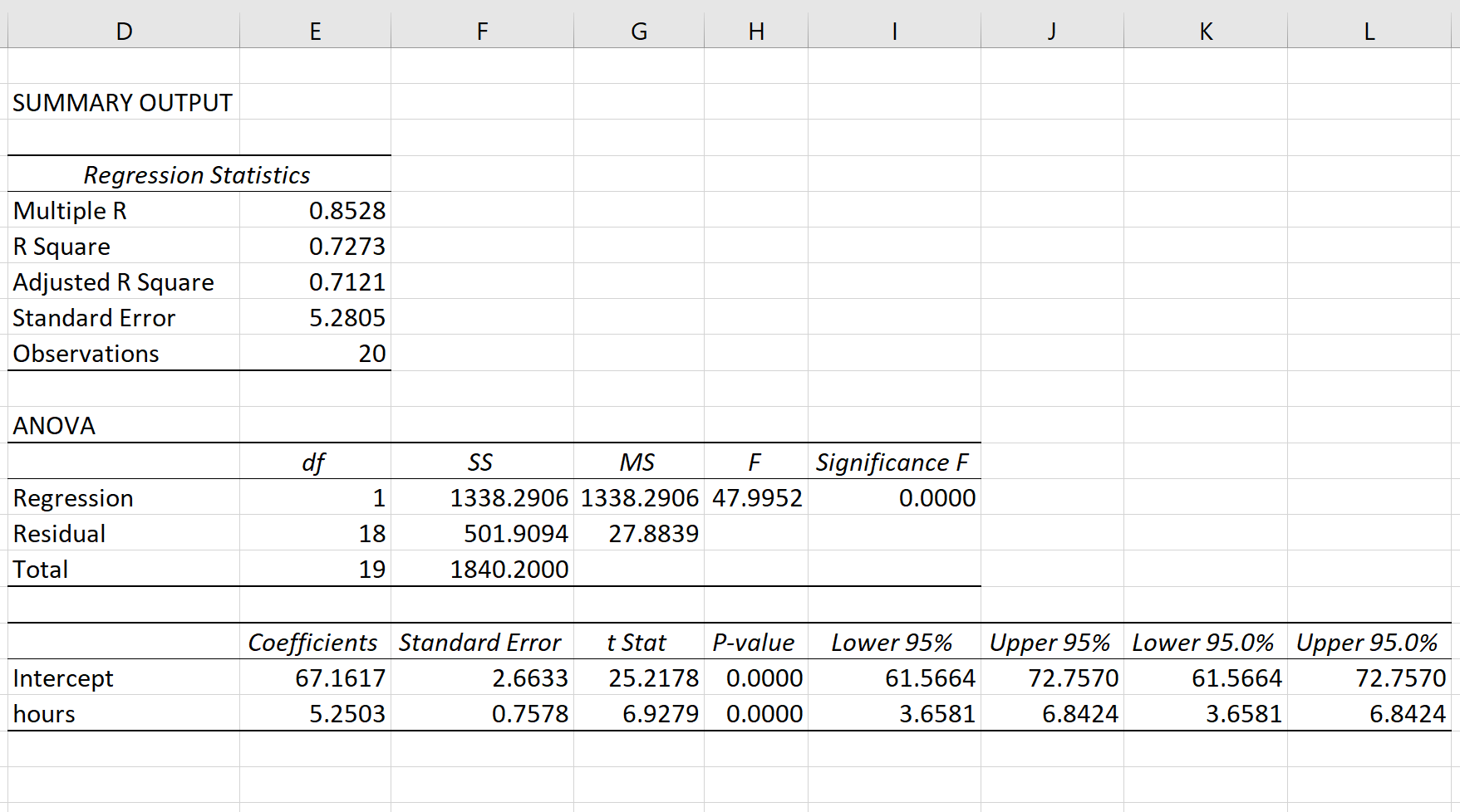
Шаг 4: Интерпретируйте вывод.
Вот как интерпретировать наиболее релевантные числа в выводе:
R-квадрат: 0,7273.Это известно как коэффициент детерминации. Это доля дисперсии переменной отклика, которая может быть объяснена объясняющей переменной. В этом примере 72,73 % различий в баллах за экзамены можно объяснить количеством часов обучения.
Стандартная ошибка: 5.2805.Это среднее расстояние, на которое наблюдаемые значения отходят от линии регрессии. В этом примере наблюдаемые значения отклоняются от линии регрессии в среднем на 5,2805 единиц.
Ф: 47,9952.Это общая F-статистика для регрессионной модели, рассчитанная как MS регрессии / остаточная MS.
Значение F: 0,0000.Это p-значение, связанное с общей статистикой F. Он говорит нам, является ли регрессионная модель статистически значимой. Другими словами, он говорит нам, имеет ли независимая переменная статистически значимую связь с переменной отклика. В этом случае p-значение меньше 0,05, что указывает на наличие статистически значимой связи между отработанными часами и полученными экзаменационными баллами.
Коэффициенты: коэффициенты дают нам числа, необходимые для написания оценочного уравнения регрессии. В этом примере оцененное уравнение регрессии:
экзаменационный балл = 67,16 + 5,2503*(часов)
Мы интерпретируем коэффициент для часов как означающий, что за каждый дополнительный час обучения ожидается увеличение экзаменационного балла в среднем на 5,2503.Мы интерпретируем коэффициент для перехвата как означающий, что ожидаемая оценка экзамена для студента, который учится без часов, составляет 67,16 .
Мы можем использовать это оценочное уравнение регрессии для расчета ожидаемого экзаменационного балла для учащегося на основе количества часов, которые он изучает.
Например, ожидается, что студент, который занимается три часа, получит на экзамене 82,91 балла:
экзаменационный балл = 67,16 + 5,2503*(3) = 82,91
Дополнительные ресурсы
В следующих руководствах объясняется, как выполнять другие распространенные задачи в Excel:
Как создать остаточный график в Excel
Как построить интервал прогнозирования в Excel
Как создать график QQ в Excel
In this tutorial, you’ll learn how to perform Linear Regression in Excel. Linear regression is an approach to linear modeling the relationship between a dependent and an independent variable. Simple linear regression uses an independent variable to predict the outcome of the dependent variable.
The equation for linear regression is given by: y = a + bx, where x is the independent variable, y is the dependent variable and the coefficients are given by:

Our aim is to find coefficients a which is the intercept and b which is the slope to obtain the equation of the straight line which best fits our data by the least square method. There are two ways in Excel in which we can find the linear regression line which is discussed below for the following data set:

Calculate Linear Regression in Excel Using Its Formula
First, we need to calculate the parameters in the formula for coefficients a and b. The parameters are Σx, Σy, Σxy and Σx2 . To calculate Σx follow these steps:
- Select the cell where you want to calculate and display the summation of x.
- Type =SUM(, select the cells containing the numbers and complete the formula with ).

- Press the Enter key to display the result.

To calculate Σy follow these steps:
- Select the cell where you want to calculate and display the summation of y.
- Type =SUM(, select the cells containing the numbers and complete the formula with ).

- Press the Enter key to display the result.

To calculate Σxy follow these steps:
- Select the cell where you want to calculate and display the product of a pair of x and y values.
- Type =B2*C2, as the first x and y values are in cells B2 and C2 respectively.

- Press the Enter key to display the result.

- Copy the formula for the calculation of product xy for the entire list by dragging down the fill handle.

- Select the cell where you want to calculate and display the summation of xy.
- Type =SUM(, select the cells containing the numbers and complete the formula with ).

- Press the Enter key to display the result.

To calculate Σx2 follow these steps:
- Select the cell where you want to calculate and display the square of the first x value.
- Type =B2^2, as the first x value, is in cell B2. The caret operator raises the number to the power written next to it.

- Press the Enter key to display the result.

- Copy the formula for the calculation of squares of x for the entire list by dragging down the fill handle.

- Select the cell where you want to calculate and display the summation of x2.
- Type =SUM(, select the cells containing the numbers and complete the formula with ).

- Press the Enter key to display the result.

We now have the parameters essential for the calculation of coefficients intercept a and slope b. Follow the steps to calculate the intercept a:
- Select the cell where you want to display the value of the intercept.
- Type =(C6*E6-B6*D6)/(4*E6-B6^2), where C6 contains the value of Σy, E6 contains the value of Σx2, B6 contains the value of Σx, D6 contains the value of Σxy and 4 is the number of data points in the data set.

- Press the Enter key to display the result.

Follow the steps to calculate the slope b:
- Select the cell where you want to display the value of the slope.
- Type =(4*D6-B6*C6)/(4*E6-B6^2), where C6 contains the value of Σy, E6 contains the value of Σx2, B6 contains the value of Σx, D6 contains the value of Σxy and 4 is the number of data points in the data set.

- Press the Enter key to display the result.

We have the values for the slope and intercept, the equation for the linear regression can be written as y = 1.5 + 0.95x. This equation can now be used to predict values of y for different values of x.
Linear Regression in Excel Using Data Analysis
To use the Data Analysis feature, you need to enable Analysis Toolpak in Excel. Follow these steps to manually enable the feature:
- Click on the File option present at the top left corner of the Excel window.
- From the menu that appears, click on Options to launch the Excel Options dialog box.
- Select the Add-ins option at the left side of the Excel Options dialog box.
- Select Excel Add-ins in the Manage box, and click Go.

- In the Add-ins dialog box, check the Analysis Toolpak checkbox, and then click OK.

- The Data Analysis option now appears in the Analysis group on the Data tab.

Follow these steps to perform linear regression using Data Analysis:
- Click on Data Analysis present in the Analysis group on the Data tab.
- From the Data Analysis dialog box that appears, select Regression under the Analysis Tools and click on OK.

- Enter the cell ranges containing y values in the Input Y Range: text box and x values in the Input X Range: text box in the Regression dialog box and click OK.

- The results are displayed in a new worksheet. You can copy the intercept and slope coefficients to obtain an equation for the linear regression: y = 1.5 + 0.95x.

Conclusion
In this tutorial, we learned how to perform linear regression both using the formulas and Excel Add-ins.
References
- Load the Analysis ToolPak in Excel – Office Support (microsoft.com)
Linear Regression in Excel (Table of Contents)
- Introduction to Linear Regression in Excel
- Methods for Using Linear Regression in Excel
Introduction to Linear Regression in Excel
Linear regression is a statistical technique/method used to study the relationship between two continuous quantitative variables. In this technique, independent variables are used to predict the value of a dependent variable. If there is only one independent variable, then it is a simple linear regression, and if a number of independent variables are more than one, then it is multiple linear regression. Linear Regression models have a relationship between dependent and independent variables by fitting a linear equation to the observed data. Linear refers to the fact that we use a line to fit our data. The dependent variables used in regression analysis are also called the response or predicted variables, and independent variables are also called explanatory variables or predictors.
A linear regression line has an equation of the kind: Y= a + bX;
Where:
- X is the explanatory variable,
- Y is the dependent variable,
- b is the slope of the line,
- a is the y-intercept (i.e. the value of y when x=0).
The least-squares method is generally used in linear regression that calculates the best fit line for observed data by minimizing the sum of squares of deviation of data points from the line.
Methods for Using Linear Regression in Excel
This example teaches you the methods to perform Linear Regression Analysis in Excel. Let’s look at a few methods.
You can download this Linear Regression Excel Template here – Linear Regression Excel Template
Method #1 – Scatter Chart with a Trendline
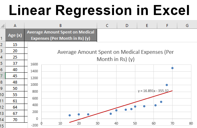
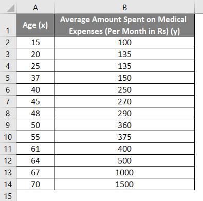
Let us say we have a dataset of some individuals with their age, bio-mass index (BMI), and the amount spent by them on medical expenses in a month. Now with an insight into the individuals’ characteristics like age and BMI, we wish to find how these variables affect the medical expenses, and hence use these to carry out regression and estimate/predict the average medical expenses for some specific individuals. Let us first see how only age affects medical expenses. Let us see the dataset:
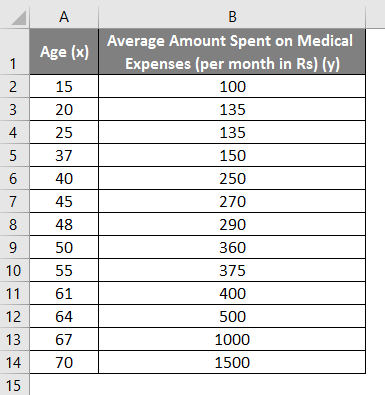
Amount on medical expenses= b*age + a
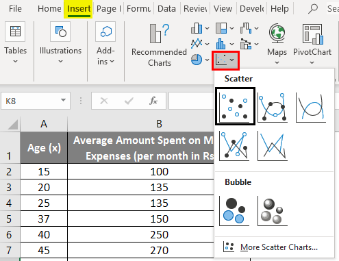
- Select the two columns of the dataset (x and y), including headers.
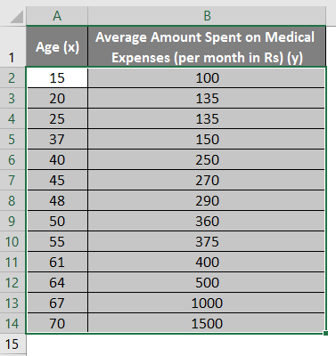
- Click on ‘Insert’ and expand the dropdown for ‘Scatter Chart’ and select ‘Scatter’ thumbnail (first one)
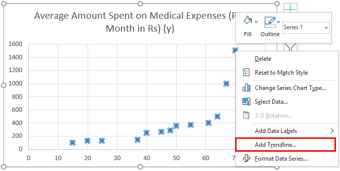
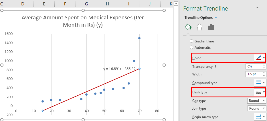
- Now a scatter plot will appear, and we would draw the regression line on this. To do this, right-click on any data point and select ‘Add Trendline.’
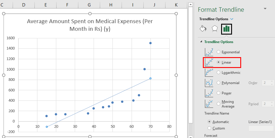
- Now in the ‘Format Trendline’ pane on the right, select ‘Linear Trendline’ and ‘Display Equation on Chart’.
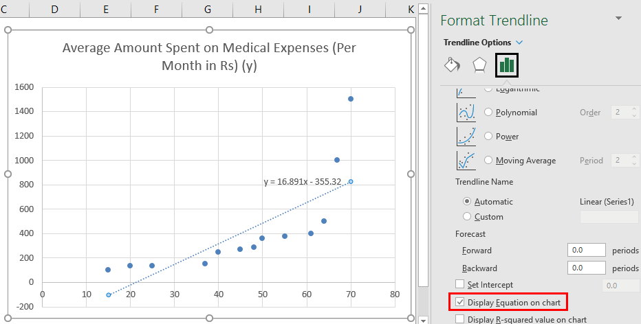
- Select ‘Display Equation on Chart’.
We can improvise the chart as per our requirements, like adding axes titles, changing the scale, color and line type.
After Improvising the chart, this is the output we get.
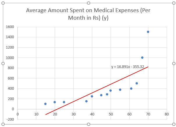
Note: In this type of regression graph, the dependent variable should always be on the y-axis and independent on the x-axis. If the graph gets plotted in reverse order, then either switch the axes in a chart or swap the columns in the dataset.
Method #2 – Analysis ToolPak Add-In Method
Analysis ToolPak is sometimes not enabled by default, and we need to do it manually. To do so:
- Click on the ‘File’ menu.
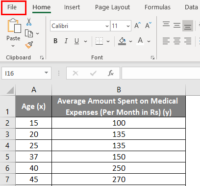
After that, click on ‘Options’.
- Select ‘Excel Add-Ins’ in the ‘Manage’ box, and click on ‘Go.’
- Select ‘Analysis ToolPak’ -> ‘OK’
This will add ‘Data Analysis’ tools to the ‘Data’ tab. Now we run the regression analysis:
- Click on ‘Data Analysis’ in the ‘Data’ tab
- Select ‘Regression’ -> ‘OK’
- A regression dialog box will appear. Select the Input Y range and Input X range (medical expenses and age, respectively). In the case of multiple linear regression, we can select more columns of independent variables (like if we wish to see the impact of BMI as well on medical expenses).
- Check the ‘Labels’ box to include headers.
- Choose the desired ‘output’ option.
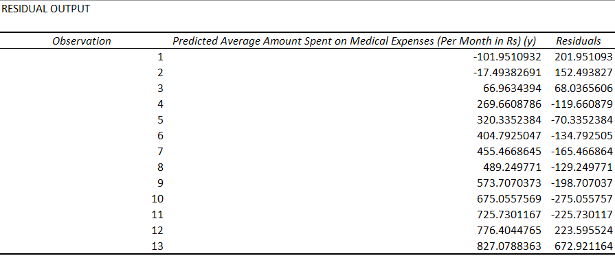
- Select the ‘residuals’ checkbox and click ‘OK.
Now our regression analysis output will be created in a new worksheet, stating the Regression Statistics, ANOVA, residuals and coefficients.
Output Interpretation:
- Regression Statistics tells how well the regression equation fits the data:
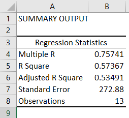
- Multiple R is the correlation coefficient that measures the strength of a linear relationship between two variables. It lies between -1 and 1, and its absolute value depicts the relationship strength with a large value indicating a stronger relationship, a low value indicating negative and zero value indicating no relationship.
- R Square is the Coefficient of Determination used as an indicator of goodness of fit. It lies between 0 and 1, with a value close to 1 indicating that the model is a good fit. In this case, 0.57=57% of y-values are explained by the x-values.
- Adjusted R Square is R Square adjusted for a number of predictors in the case of multiple linear regression.
- Standard Error depicts the precision of regression analysis.
- Observations depict the number of model observations.
- Anova tells the level of variability within the regression model.
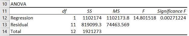
This is generally not used for simple linear regression. However, the ‘Significance F values’ indicate how reliable our results are, with a value greater than 0.05 suggesting to choose another predictor.
- Coefficients are the most important part used to build regression equation.

So, our regression equation would be: y= 16.891 x – 355.32. This is the same as that done by method 1 (scatter chart with a trendline).
Now, if we wish to predict average medical expenses when age is 72:
So y= 16.891 * 72 -355.32 = 860.832
So this way, we can predict values of y for any other values of x.
- Residuals indicate the difference between actual and predicted values.
The last method for regression is not so commonly used and requires statistical functions like slope (), intercept (), correl (), etc., to carry out regression analysis.
Things to Remember About Linear Regression in Excel
- Regression analysis is generally used to see if there is a statistically significant relationship between two sets of variables.
- It is used to predict the value of the dependent variable based on the values of one or more independent variables.
- Whenever we wish to fit a linear regression model to a group of data, then the range of data should be carefully observed. If we use a regression equation to predict any value outside this range (extrapolation), it may lead to wrong results.
Recommended Articles
This is a guide to Linear Regression in Excel. Here we discuss how to do Linear Regression in Excel along with practical examples and a downloadable excel template. You can also go through our other suggested articles –
- Excel Regression Analysis
- Linear Programming in Excel
- Linear Interpolation in Excel
- Statistics in Excel