
Excel for Microsoft 365 Excel for Microsoft 365 for Mac Excel for the web Excel 2021 Excel 2021 for Mac Excel 2019 Excel 2019 for Mac Excel 2016 Excel 2016 for Mac Excel 2013 Excel 2010 Excel 2007 Excel for Mac 2011 More…Less
Multiplying and dividing in Excel is easy, but you need to create a simple formula to do it. Just remember that all formulas in Excel begin with an equal sign (=), and you can use the formula bar to create them.
Multiply numbers
Let’s say you want to figure out how much bottled water that you need for a customer conference (total attendees × 4 days × 3 bottles per day) or the reimbursement travel cost for a business trip (total miles × 0.46). There are several ways to multiply numbers.
Multiply numbers in a cell
To do this task, use the * (asterisk) arithmetic operator.
For example, if you type =5*10 in a cell, the cell displays the result, 50.
Multiply a column of numbers by a constant number
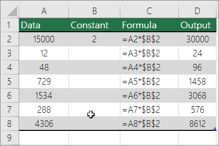
Suppose you want to multiply each cell in a column of seven numbers by a number that is contained in another cell. In this example, the number you want to multiply by is 3, contained in cell C2.
-
Type =A2*$B$2 in a new column in your spreadsheet (the above example uses column D). Be sure to include a $ symbol before B and before 2 in the formula, and press ENTER.
Note: Using $ symbols tells Excel that the reference to B2 is «absolute,» which means that when you copy the formula to another cell, the reference will always be to cell B2. If you didn’t use $ symbols in the formula and you dragged the formula down to cell B3, Excel would change the formula to =A3*C3, which wouldn’t work, because there is no value in B3.
-
Drag the formula down to the other cells in the column.
Note: In Excel 2016 for Windows, the cells are populated automatically.
Multiply numbers in different cells by using a formula
You can use the PRODUCT function to multiply numbers, cells, and ranges.
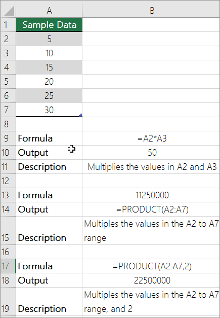
You can use any combination of up to 255 numbers or cell references in the PRODUCT function. For example, the formula =PRODUCT(A2,A4:A15,12,E3:E5,150,G4,H4:J6) multiplies two single cells (A2 and G4), two numbers (12 and 150), and three ranges (A4:A15, E3:E5, and H4:J6).
Divide numbers
Let’s say you want to find out how many person hours it took to finish a project (total project hours ÷ total people on project) or the actual miles per gallon rate for your recent cross-country trip (total miles ÷ total gallons). There are several ways to divide numbers.
Divide numbers in a cell
To do this task, use the / (forward slash) arithmetic operator.
For example, if you type =10/5 in a cell, the cell displays 2.
Important: Be sure to type an equal sign (=) in the cell before you type the numbers and the / operator; otherwise, Excel will interpret what you type as a date. For example, if you type 7/30, Excel may display 30-Jul in the cell. Or, if you type 12/36, Excel will first convert that value to 12/1/1936 and display 1-Dec in the cell.
Note: There is no DIVIDE function in Excel.
Divide numbers by using cell references
Instead of typing numbers directly in a formula, you can use cell references, such as A2 and A3, to refer to the numbers that you want to divide and divide by.
Example:
The example may be easier to understand if you copy it to a blank worksheet.
How to copy an example
-
Create a blank workbook or worksheet.
-
Select the example in the Help topic.
Note: Do not select the row or column headers.

Selecting an example from Help
-
Press CTRL+C.
-
In the worksheet, select cell A1, and press CTRL+V.
-
To switch between viewing the results and viewing the formulas that return the results, press CTRL+` (grave accent), or on the Formulas tab, click the Show Formulas button.

|
A |
B |
C |
|
|
1 |
Data |
Formula |
Description (Result) |
|
2 |
15000 |
=A2/A3 |
Divides 15000 by 12 (1250) |
|
3 |
12 |
Divide a column of numbers by a constant number
Suppose you want to divide each cell in a column of seven numbers by a number that is contained in another cell. In this example, the number you want to divide by is 3, contained in cell C2.
|
A |
B |
C |
|
|
1 |
Data |
Formula |
Constant |
|
2 |
15000 |
=A2/$C$2 |
3 |
|
3 |
12 |
=A3/$C$2 |
|
|
4 |
48 |
=A4/$C$2 |
|
|
5 |
729 |
=A5/$C$2 |
|
|
6 |
1534 |
=A6/$C$2 |
|
|
7 |
288 |
=A7/$C$2 |
|
|
8 |
4306 |
=A8/$C$2 |
-
Type =A2/$C$2 in cell B2. Be sure to include a $ symbol before C and before 2 in the formula.
-
Drag the formula in B2 down to the other cells in column B.
Note: Using $ symbols tells Excel that the reference to C2 is «absolute,» which means that when you copy the formula to another cell, the reference will always be to cell C2. If you didn’t use $ symbols in the formula and you dragged the formula down to cell B3, Excel would change the formula to =A3/C3, which wouldn’t work, because there is no value in C3.
Need more help?
You can always ask an expert in the Excel Tech Community or get support in the Answers community.
See Also
Multiply a column of numbers by the same number
Multiply by a percentage
Create a multiplication table
Calculation operators and order of operations
Need more help?
Want more options?
Explore subscription benefits, browse training courses, learn how to secure your device, and more.
Communities help you ask and answer questions, give feedback, and hear from experts with rich knowledge.
![]()
Download Article
An easy-to-use guide to multiply numbers in Excel automatically
![]()
Download Article
This wikiHow teaches you how to multiply numbers in Excel. You can multiply two or more numbers within one Excel cell, or you can multiply two or more Excel cells against one another.
-
1
Open Excel. It’s a green app with a white «X» on it.
- You’ll need to click Blank workbook (PC) or New and then Blank Workbook (Mac) to continue.
- If you have an existing presentation you’d like to open, double-click it to open it in Excel.
-
2
Click a cell. Doing so will select it, allowing you to type into it.
Advertisement
-
3
Type = into the cell. All formulas in Excel start with the equals sign.
-
4
Enter the first number. This should go directly after the «=» symbol with no space.
-
5
Type * after the first number. The asterisk symbol indicates that you wish to multiply the number before the asterisk with the number that comes after it.
-
6
Enter the second number. For example, if you first entered a 6, and wanted to multiply it by 6, your formula would now look like =6*6.
- You can repeat this process with as many numbers as you like, as long as the «*» symbol is between each of the numbers you want to multiply.
-
7
Press ↵ Enter. This will run your formula. The cell will display the product of the formula, though clicking the cell will display the formula itself in the Excel address bar.


Advertisement
-
1
Open an Excel presentation. Simply double-click an Excel document to open it in Excel.
-
2
Click a cell. Doing so will select it, allowing you to type into it.
-
3
Type = into the cell. All formulas in Excel start with the equals sign.
-
4
Type in another cell’s name. This should go directly after the «=» with no space.
- For example, typing «A1» into the cell sets A1’s value as the first number in your formula.
-
5
Type * after the first cell name. The asterisk symbol indicates to Excel that you want to multiply the value before it with the value after it.
-
6
Type in a different cell’s name. This will set the second variable in your formula as the second cell’s value.
- For example, typing «D5» into the cell would make your formula look like this:
=A1*D5. - You can add more than two cell names to this formula, though you’ll need to type «*» between subsequent cell names.
- For example, typing «D5» into the cell would make your formula look like this:
-
7
Press ↵ Enter. This will run your formula and display the result in your selected cell.
- When you click the cell with the formula result, the formula itself will display in the Excel address bar.


Advertisement
-
1
Open an Excel presentation. Simply double-click an Excel document to open it in Excel.
-
2
Click a cell. Doing so will select it, allowing you to type into it.
-
3
Type =PRODUCT( into your cell. This command indicates that you want to multiply items together.
-
4
Type in the first cell’s name. This should be the cell at the top of the range of data.
- For example, you might type «A1» here.
-
5
Type : . The colon symbol («:») indicates to Excel that you want to multiply everything from the first cell through the next cell you enter.
-
6
Type in another cell’s name. This cell must be in the same column or row as the first cell in the formula if you want to multiply all the cells from the first cell to this one.
- In the example, typing «A5» would set up the formula to multiply the contents of A1, A2, A3, A4, and A5 together.
-
7
Type ), then press ↵ Enter. This last parenthesis closes the formula, and hitting enter runs the command and multiplies your range of cells together, displaying the result instantly in your selected cell.
- If you change the contents of a cell within the multiplication range, the value in your selected cell will also change.


Advertisement
Add New Question
-
Question
How can I multiply two columns together?

In another column, create a formula by entering =, then selecting the first value and typing * (which means multiply) before selecting the second value and pressing enter.
-
Question
How would I multiply 0.5 by a number, such as $37.50?
In any cell, you would simply enter = 0.5 * 37.5. As you leave the cell, the answer will be displayed. Alternatively, put 0.5 into cell A1 and 37.5 into cell A2. In cell A3, type = A1*A2. When you press Enter, the answer will be displayed.
-
Question
When I multiply two numbers, why do they disappear when the product shows up?
Excel will only show the product. If you also want to see the numbers you multiplied, you will have to write them again.
See more answers
Ask a Question
200 characters left
Include your email address to get a message when this question is answered.
Submit
Advertisement
Video
-
When using the PRODUCT formula to calculate the product of a range, you can select more than just one column or row. For example, your range could be =PRODUCT(A1:D8). This will multiply all of the values of the cells in the rectangle defined by the range (A1-A8, B1-B8, C1-C8, D1-D8).
Thanks for submitting a tip for review!
Advertisement
About This Article
Article SummaryX
Two numbers in a cell:
1. Type = into a cell.
2. Type the first number.
3. Type *.
4. Type the second number.
5. Press Enter or Return.
Two cells:
1. Type = into a cell.
2. Click the first cell value.
3. Type *.
4. Click the second cell value.
5. Press Enter or Return.
Did this summary help you?
Thanks to all authors for creating a page that has been read 691,679 times.
Reader Success Stories
-

«Recently-retired exec who has had really good admin assistants for years, and I needed refresher on formulas. This…» more
Is this article up to date?
- You can multiply in Excel using a few different methods.
- It’s easy to multiply two numbers in Excel, but you can also multiply many different cells and numbers together, or multiply a column of values by a constant.
- Visit Business Insider’s homepage for more stories.
Multiplying values is one of the most frequently performed functions in Excel, so it should be no surprise that there are several ways to do this.
You can use whichever method is best suited to what you are trying to accomplish in your spreadsheet on a Mac or PC.
Here are a few of your simplest options to perform multiplication.
Check out the products mentioned in this article:
Microsoft Office 365 Home (From $99.99 at Best Buy)
MacBook Pro (From $1,299.99 at Best Buy)
Lenovo IdeaPad 130 (From $299.99 at Best Buy)
How to multiply two numbers in Excel
The easiest way to do this is by multiplying numbers in a single cell using a simple formula.
For example, if you type «=2*6» into a cell and press Enter on the keyboard, you should see the cell display «12.»
Dave Johnson/Business Insider
You can also multiply two different cells together.
1. In a cell, type «=»
2. Click in the cell that contains the first number you want to multiply.
3. Type «*».
4. Click the second cell you want to multiply.
5. Press Enter.
Dave Johnson/Business Insider
How to multiply cells and numbers using the PRODUCT formula
You aren’t limited to multiplying just two cells — you can multiply up to 255 values at once using the PRODUCT formula.
Using this formula, you can multiply individual cells and numbers by separating them with commas and multiply a series of cells with a colon.
For example, in the formula «=PRODUCT(A1,A3:A5,B1,10)» — Excel would multiply (A1 x A3 x A4 x A5 x B1 x 10) because A3:A5 indicates that it should multiply A3, A4, and A5.
Remember that the order of these cells and numbers is irrelevant in multiplication.
How to multiply a column of values by a constant
Suppose you have a series of numbers and want to multiply each one of them by the same value. You can do that by using an absolute reference to the cell that contains the constant.
1. Set up a column of numbers you want to multiply, and then put the constant in another cell.
2. In a new cell, type «=» and click the first cell you want to multiply.
3. Type the name of the cell that contains the constant, adding a «$» before both the letter and number. The dollar sign turns this into an absolute reference, so it won’t change if you copy and paste it in the spreadsheet.
Dave Johnson/Business Insider
4. Press Enter.
5. You can now copy and paste this to additional cells to perform the multiplication on the other numbers. The easiest way to do this is to drag the cell by its lower right corner to copy it.
Dave Johnson/Business Insider
Related coverage from How To Do Everything: Tech:
-
How to merge and unmerge cells in Microsoft Excel in 4 ways, to clean up your data and formatting
-
How to lock cells in Microsoft Excel, so people you send spreadsheets to can’t change certain cells or data
-
How to alphabetize data in an Excel spreadsheet by column or row, and by using shortcuts
-
How to embed a YouTube video into a PowerPoint presentation, depending on the version of your PowerPoint
Dave Johnson
Freelance Writer
Dave Johnson is a technology journalist who writes about consumer tech and how the industry is transforming the speculative world of science fiction into modern-day real life. Dave grew up in New Jersey before entering the Air Force to operate satellites, teach space operations, and do space launch planning. He then spent eight years as a content lead on the Windows team at Microsoft. As a photographer, Dave has photographed wolves in their natural environment; he’s also a scuba instructor and co-host of several podcasts. Dave is the author of more than two dozen books and has contributed to many sites and publications including CNET, Forbes, PC World, How To Geek, and Insider.
Read more
Read less
Here are several ways how to multiply in excel. We are providing a guide on the best ways of multiplication in excel. Follow and get your best appropriate way. To make the most straightforward multiplication formula in Excel, type the equals sign (=) in a cell, then type the first number you want to multiply, followed by an asterisk, accompanied by the second number, and hit the Enter key to add the formula.
For instance, to multiply 2 by 5, you write this expression in a cell (with no spaces): =2*5
Excel allows showing different arithmetic operations within one formula. Just learn about the order of calculations (PEMDAS): parentheses, multiplication, exponentiation, or division, whichever comes first, addition, or subtraction, whichever occurs first.
If you encounter troubles while working with Excel tables, one of the common reasons is the .xlsx file corruption. The Excel repair software is able to deal with this sort of problem with ease and allows the user to continue working with Excel files properly.
How to Multiply Cells in MSExcel
To multiply two Excel cells, use a multiplication formula like in the above example, but supply cell references instead of numbers. For instance, to multiply the value in cell A2 by the value in B2, write this expression:
=A2*B2
To multiply multiple cells, involve more cell references in the formula, separated by the multiplication sign. For example:
=A2*B2*C2
How to Multiply Columns in Excel
To multiply two columns in MSExcel, type the multiplication formula for the topmost cell, for instance:
=A2*B2
After you’ve set the formula in the first cell (C2 in this example), double-click the small green square in the lower-right corner of the cell to copy the formula down the column, up to the end cell with data:
Due to the use of relative cell references (without the $ sign), our MSExcel multiply formula will adjust appropriately for each row.
In my view, this is the best but not the only approach to multiplying one column by another. You can learn other entrances in this tutorial: How to multiply columns in MSExcel.
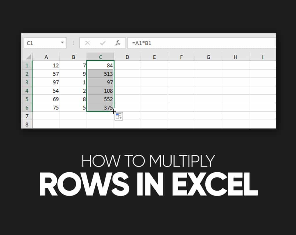
How to Multiply Rows in Excel
Multiplying rows in Excel is a less familiar task, but there is a simple solution for it too. To multiply two rows in MSExcel, do the following:
- Enter a multiplication formula in the first (leftmost) cell.
- In this example, we multiply values in row 1 by the values in row 2, beginning with column B. So our formula goes as follows: =B1*B2
- Choose the formula cell, and hover the mouse cursor over a little square at the lower right-hand corner until it changes to a thick black cross.
- Pull that black cross rightward over the cells where you need to copy the formula.
As with multiplying columns, the corresponding cell references in the formula change based on a relative position of rows and columns, multiplying a value in row 1 by a value in row 2 in each column.
How to Multiply in MSExcel – Multiply Function in Excel (PRODUCT)
If you want to multiply multiple cells or ranges, the fastest method would be using the PRODUCT function:
PRODUCT(number1, [number2], …)
Where number1, number2, etc. are numbers, cells, or areas that you need to multiply.
For instance, to multiply values in cells A2, B2, and C2, apply this formula:
=PRODUCT(A2:C2)
To multiply the figures in cells A2 through C2, and then multiply the outcome by 3, use this one:
=PRODUCT(A2:C2,3)
Multiply Numbers in Excel by Using the Product Formula
You can use the basic formula to cross multiply the numbers in MSexcel if you use the product formula to multiply up to 255 values at once.
- So, First, go to MS Excel and choose any blank cell. Then type an equal symbol, followed by the word PRODUCT. Next, add an opening addition.
- Multiply Individual Cells, type the names of the cells and divide them with commas without space.
- To Multiply a Series of Cells, type a colon between two cells’ names to specify that all cells within that range should be multiplied. For instance, “=PRODUCT(A2:A5)” point out that cells A2,A3, A4, and A5 should be multiplied.
- If you want to add a number to the equation, so enter a comma and then that number.
- When you complete entering the Values of your formula, then put a closing Parenthesis at last and hit the “Enter” button on your Keyboard. The equation answer will all show in the cell.
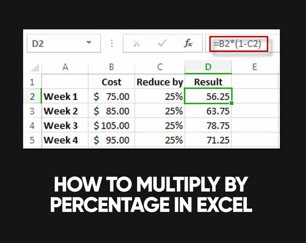
How to Multiply by Percentage in Excel
To multiply percentages in MSExcel, do a multiplication formula in this way: type the equals sign, followed by the number or cell, followed by the multiply sign (*), followed by a percentage.
In other terms, make a formula similar to these:
- To multiply a number by percentage: =50*10%
- To multiply a cell by percentage: =A1*10%
Rather than percentages, you can multiply by a similar decimal number. For example, knowing that 10 percent is ten parts of a hundred (0.1), use the following expression to multiply 50 by 10%: =50*0.1
How to Multiply a Column by a Number in the Excel
To multiply a column of numbers by the corresponding number, proceed with these steps:
- Insert the number to multiply by in some cell, say in A2.
- Type a multiplication formula for the topmost cell in the column.
- Considering the numbers to be multiplied are in column C, beginning in row 2. You set the following formula in D2:
- =C2*$A$2
- You must lock the column and row coordinates of the cell with the number to multiply by to prevent the reference from changing when you copy the formula to other cells. For this, type the $ symbol before the column letter and row number to make an absolute reference ($A$2). Or, click on the reference and press the F4 key to change it to complete.
- Double-click enough handle in the formula cell (D2) to copy the formula down the column. Done!
C2 (relative reference) changes to C3 when the formula is copied to row 3, while $A$2 (absolute reference) continues unchanged:
If the design of your worksheet does not provide an additional cell to accommodate the number, you can supply it directly in the formula, e.g., =C2*3
You can also apply the Paste Special > multiply feature to multiply a column by a constant number and get the results as values rather than formulas. Please check out this example for detailed instructions.
How to Multiply and Sum in Excel
When you require to multiply two columns or rows of numbers, and then add up the results of different calculations, use the SUMPRODUCT function to multiply cells and sum products.
Assuming you have prices in column B, quantity in column C, and calculate the total value of sales. In your math class, you’d multiply each Price/Qty. Pair individually and add up the sub-totals.
In Microsoft Excel, all these computations can be done with a single formula:
=SUMPRODUCT(B2:B5,C2:C5)
If you want, you can check the outcome with this calculation:
=(B2*C2)+(B3*C3)+(B4*C4)+(B5*C5)
And make assured the SUMPRODUCT formula multiplies and sums correctly:
Multiplication in Array Formulas
In case you want to multiply two columns of numbers and then perform further calculations with the results. Do multiplication within an array formula.
In the higher data set, another way to calculate the total value of sales is this:
=SUM(B2:B5*C2:C5)
This Excel Sum Multiply formula is equivalent to SUMPRODUCT and returns precisely the same result.
Taking the case further, let’s find an average sales. For this, use the AVERAGE function instead of SUM:
=AVERAGE(B2:B5*C2:C5)
To find the most extensive and smallest sale, use the MAX and MIN functions, respectively:
=MAX(B2:B5*C2:C5)
=MIN(B2:B5*C2:C5)
To complete an array formula correctly, be sure to press the Ctrl + Shift + Enter combination instead of entering a stroke. As quickly as you do this, Excel will enclose the formula in {curly braces}, indicating it’s an array formula.
Conclusion
Suppose you belong to any organization or company. In that case, this guide will be helpful for you because it includes all the multiplication methods and it means a lot to every organizational person. Multiplication in excel is not as difficult as you think. But if you want to do it quickly, you must memorize the formula to convert the complex method into an easy method. Let us know how much the excel sheet is helpful for you.
There is no in-built multiplication formula in Excel. Multiplication in excel is performed by entering the comparison operator “equal to” (=), followed by the first number, the “asterisk” (*), and the second number. In this way, it is possible to carry out the multiplication operation for a cell, row or column. For example, the formula “=16*3*2” multiplies the numbers 16, 3, and 2. It returns 96.
The arithmetic operator “asterisk” (*) is known as the multiplication symbol. It is placed between the numbers to be multiplied.
In multiplication, the number to be multiplied is known as the multiplicand. The number by which the multiplicand is multiplied is known as the multiplier. The multiplier and the multiplicand are also called factors. Their output of multiplication is known as the product.
In Excel, multiplication can be performed in the following ways:
- With the “asterisk” symbol (*)
- With the PRODUCT functionProduct excel function is an inbuilt mathematical function which is used to calculate the product or multiplication of the given numbers. If you provide this formula arguments as 2 and 3 as =PRODUCT(2,3) then the result displayed is 6.read more
- With the SUMPRODUCT functionThe SUMPRODUCT excel function multiplies the numbers of two or more arrays and sums up the resulting products.read more
Note: The SUMPRODUCT function multiplies and then sums the resulting products.
Table of contents
- How to Use Multiply Formula in Excel?
- Example #1 – Multiply Excel Columns With the “Asterisk”
- Example #2 – Multiply Excel Rows With the “Asterisk”
- Example #3 – Multiply With the PRODUCT Function
- Example #4 – Multiply and Sum With the SUMPRODUCT Function
- Example #5 – Multiply With Percentages
- Frequently Asked Questions
- Recommended Articles
How to Use Multiply Formula in Excel?
You can download this Multiply Function Excel Template here – Multiply Function Excel Template
Example #1 – Multiply Excel Columns With the “Asterisk”
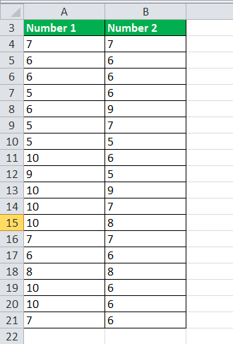
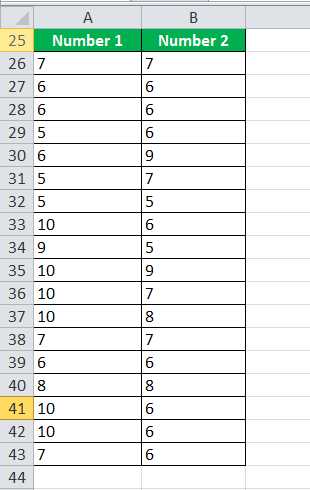
The following table shows two columns titled “number 1” and “number 2.” We want to multiply the numerical values of the first column by the second one.
Step 1: Enter the multiplication formula in excel “=A4*B4” in cell C4.
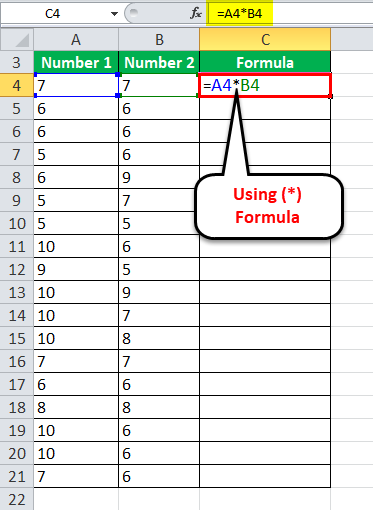
Step 2: Press the “Enter” key. The output is 49, as shown in the succeeding image. Drag or copy-paste the formula to the remaining cells.
For simplicity, we have retained the formulas in column C and given the products in column D.

Example #2 – Multiply Excel Rows With the “Asterisk”
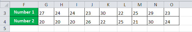
The following table shows two rows titled “number 1” and “number 2.” We want to multiply the numerical values of the first row by the second one.
Step 1: Enter the multiplication formula “=G3*G4” in cell G5.
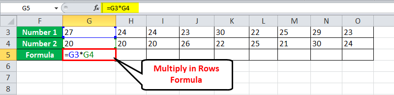
Step 2: Press the “Enter” key. The output is 540, as shown in the succeeding image. Drag or copy-paste the formula to the remaining cells.
For simplicity, we have retained the formulas in row 5 and given the products in row 6.

Example #3 – Multiply With the PRODUCT Function
The PRODUCT function can be given a list of numbers as arguments to be multiplied.
Working on the data of example #1, we want to multiply the numerical values of the two columns with the help of the PRODUCT function.
Step 1: Enter the formula “=PRODUCT (A26,B26)” in cell C26.

Step 2: Press the “Enter” key. The output is 49, as shown in the succeeding image. Drag or copy-paste the formula to the remaining cells.
For simplicity, we have retained the formulas in column C and given the products in column D.

Example #4 – Multiply and Sum With the SUMPRODUCT Function
With the SUMPRODUCT function, the numbers of two columns or rows are multiplied and the resulting products are summed up.
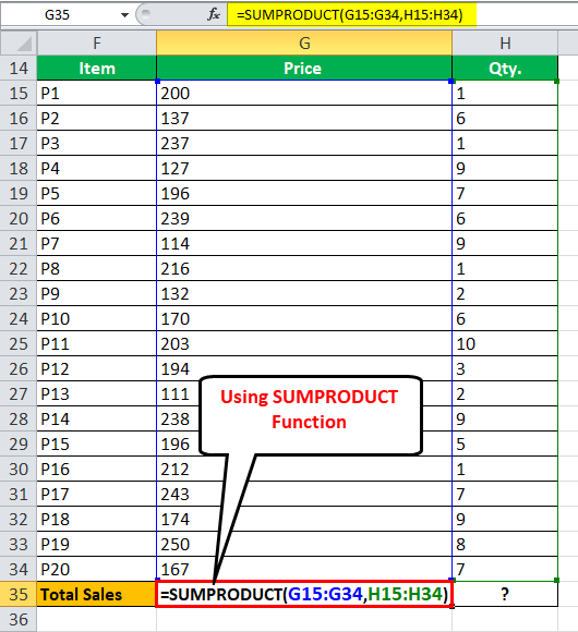
The following table shows the prices (in $ per unit) and quantities sold of 20 items. We want to calculate the total sales revenue generated by the organization.

Step 1: Enter the formula “=SUMPRODUCT (G15:G34,H15:H34).”
To calculate the sales revenue, the prices are multiplied by the quantity sold. Thereafter, the resulting products are added by the given formula.
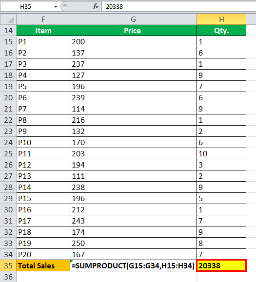
Step 2: Press the “Enter” key. The output is $20,338.
For simplicity, we have retained the formula in cell G35 and given the result in cell H35.
Example #5 – Multiply With Percentages
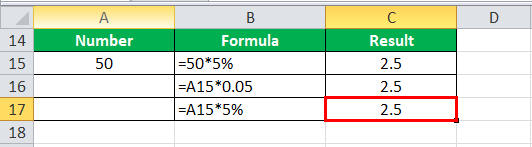
The following table shows a number in column A. We want to multiply this by 5%.
Step 1: Enter any of the following three formulas:
- “=50*5%”
- “=A15*0.05”
- “=A15*5%”

Step 2: Press the “Enter” key. The output is 2.5 with all the three formulas. It is shown in the following image.
For simplicity, we have retained the formulas in column B and given the results in column C.
Frequently Asked Questions
1. What is the multiplication formula and how to multiply in Excel?
There is no universal formula for multiplication in Excel. However, Excel facilitates multiplication with the use of the “asterisk” (*) and the PRODUCT function.
The formula using the “asterisk” is stated as follows:
“=number 1*number 2”
This is the simplest approach to multiplication that helps multiply numbers, cell references, rows, and columns.
The syntax using the PRODUCT function is stated as follows:
“=PRODUCT(number1,[number2], …)”
The “number1” and “number2” arguments can be in the form of numbers, cell references or ranges. Only the “number1” argument is required.
The steps to multiply in Excel are listed as follows:
• Enter the comparison operator “equal to” (=).
• Enter the multiplication formula.
• Press the “Enter” key to obtain the output.
Note: A maximum of 255 arguments can be provided to the PRODUCT function.
2. How to multiply in Excel without using the formula?
Let us multiply the numbers 4, 15, 23, and 54 (in the range A2:A5) by the constant 2 (in cell B2) without using the formula.
The steps to multiply in excel with “paste special” are listed as follows:
• Select cell B2 and press the keys “Ctrl+C” to copy it.
• Select the range A2:A5, which is to be multiplied.
• Right-click the selected range and choose “paste special.”
• In the “paste special” window, select “multiply” under “operation.”
• Click “Ok.”
The outputs 8, 30, 46, and 108 are obtained in the range A2:A5.
Note: If you do not want the range A2:A5 to be overridden with new values, copy-paste the numbers of this range to a separate column. This is to be done at the beginning of the mentioned procedure.
3. How to multiply two columns in Excel?
Let us multiply column A consisting of 5, 18, 26, and 44 (in the range A2:A5) by column B consisting of 6, 4, 9, and 2 (in the range B2:B5).
The steps to multiply two columns in excel using the multiplication symbol or the PRODUCT formula are listed as follows:
• Enter the formula “=A2*B2” or “=PRODUCT(A2,B2)” in cell C2.
• Press the “Enter” key. The output 30 appears in cell C2.
• Drag or copy-paste the formula to the remaining cells.
The outputs 30, 72, 234, and 88 are obtained in the range C2:C5.
Note: Since relative references are being used, the cell reference changes as the formula is copied.
The steps to multiply two excel columns using the array formula are listed as follows:
• Select the entire range C2:C5 where you want the output.
• Enter the formula “=A2:A5*B2:B5” in the selected range.
• Press the keys “Ctrl+Shift+Enter” together. The curly braces {} appear in the formula bar.
The outputs 30, 72, 234, and 88 are obtained in the range C2:C5.
Recommended Articles
This has been a guide to the multiply formula of Excel. Here we discuss how to multiply numbers, rows, columns, and percentages in Excel. We also discussed the usage of the PRODUCT and the SUMPRODUCT function of Excel. You may learn more about Excel from the following articles-
- SUMIFS With Multiple Criteria
- Formula Grade in ExcelThe Grade system formula is actually a nested IF formula in excel that checks certain conditions and returns the particular Grade if the condition is met. It is developed to check all conditions we have for the grade slab, and the grade that belongs to the condition is returned. read more
- SUMPRODUCT with Multiple CriteriaIn Excel, using SUMPRODUCT with several Criteria allows you to compare different arrays using multiple criteria.read more
- Excel Percentage Change FormulaA percentage change formula in excel evaluates the rate of change from one value to another. It is computed as the percentage value of dividing the difference between current and previous values by the previous value.read more
- Compare Two Lists in ExcelThe five different methods used to compare two lists of a column in excel are — Compare Two Lists Using Equal Sign Operator, Match Data by Using Row Difference Technique, Match Row Difference by Using IF Condition, Match Data Even If There is a Row Difference, Partial Matching Technique.read more
To multiply numbers in Excel, use the asterisk symbol (*) or the PRODUCT function. Learn how to multiply columns and how to multiply a column by a constant.
1. The formula below multiplies numbers in a cell. Simply use the asterisk symbol (*) as the multiplication operator. Don’t forget, always start a formula with an equal sign (=).

2. The formula below multiplies the values in cells A1, A2 and A3.

3. As you can imagine, this formula can get quite long. Use the PRODUCT function to shorten your formula. For example, the PRODUCT function below multiplies the values in the range A1:A7.

4. Here’s another example.

Explanation: =A1*A2*A3*A4*A5*A6*A7*B1*B2*B3*B4*C1*8 produces the exact same result.
Take a look at the screenshot below. To multiply two columns together, execute the following steps.
5a. First, multiply the value in cell A1 by the value in cell B1.

5b. Next, select cell C1, click on the lower right corner of cell C1 and drag it down to cell C6.

Take a look at the screenshot below. To multiply a column of numbers by a constant number, execute the following steps.
6a. First, multiply the value in cell A1 by the value in cell A8. Fix the reference to cell A8 by placing a $ symbol in front of the column letter and row number ($A$8).

6b. Next, select cell B1, click on the lower right corner of cell B1 and drag it down to cell B6.

Explanation: when we drag the formula down, the absolute reference ($A$8) stays the same, while the relative reference (A1) changes to A2, A3, A4, etc.
If you’re not a formula hero, use Paste Special to multiply in Excel without using formulas!
7. For example, select cell C1.

8. Right click, and then click Copy (or press CTRL + c).
9. Select the range A1:A6.
10. Right click, and then click Paste Special.
11. Click Multiply.

12. Click OK.

Note: to multiply numbers in one column by numbers in another column, at step 7, simply select a range instead of a cell.
Disclosure: Some of the links on this site are affiliate links, meaning that if you click on one of the links and purchase an item, I may receive a commission. All opinions however are my own.
One of the basic mathematic operations which we wildly use in our day-to-day life is multiplication. We all know how to multiply in our notebooks but do you know how to multiply in excel?? Yes, we can easily multiply in excel using simple multiplication formulas.
The multiplication formula in excel is extremely easy to apply and we will tell you how.
In this tutorial, we will walk you through the step-by-step guide on how to multiply on excel, just stay tuned and read along!
How To Multiply In Excel:
There are several ways you can do multiplication on excel. All of them are really easy and hardly involve any tough steps.
If you have been following other guides on this blog, you might have learned so far how to apply different formulas on excel. If you have not gone through the other excel guides yet, click here.
My point for referring you to those articles was to let you know that there are two ways you can apply the excel multiplication formula. The first method is by using the values of the cell while the other method is by using the cell reference.
Using the above two methods you can multiply the values, you can multiply the product of two cells to any number and there are many other kinds of multiplications you can perform on excel.
So let’s figure out how to multiply cells in excel in different ways using various formulas.
#Multiplying two cells by a simple formula:
The simplest multiplication we know is by multiplying two or more values with each other and this is the easiest multiplication we do on excel.
To do such a calculation, open the excel sheet with two or more cells filled with values to be multiplied. In our case, it’s the cell ‘A’ and ‘B’ which we want to multiply to each other and we want the result in Cell ‘C’.

Now if you have been ever working on excel, you might know that every formula in excel begins with an equal(=) operator. And we apply this formula to the cell where we want the result to appear. So we will apply the formula in cell “C” since we want the result there.
The formula which we will apply for multiplication in excel is Cell1*Cell2, the asterisk ( * ) is the multiplication operator. So use it between the cell values to get your results.
So the formula should look like = A1 * B1. See the below screenshot to understand how to apply this formula to multiply two numbers or cell values in excel.

Once you have written the formula, just press enters and see your result. Now click on the results cell and drag it up to the last value in the column or the cell you want the multiplication to be done.
To multiply more than two values or columns, you don’t need to put in the extra effort. Just write the third value post *. The formula will become = A1 * B1*C1.
Note: To avoid any confusion while writing down the cell address, you can simply click on the cell you want to write down. For instance, we wanted the result in cell C.
Instead of writing down cell name i.e A1, B1, etc manually, write = in column C( Formula starts with the equal operator in excel), now move your cursor and select the cell you wanted to write down i.e A1.
Now write the multiplication operator and select cell B1 and so on. By selecting I mean by clicking on the cell. This way won’t require writing the cell name manually. Hence, you won’t make any mistakes.
#Multiplying a range of cells:
Now suppose you don’t have to multiply one, two, or three columns but a range of columns i.e from A to D. So instead of writing the cell name manually, you can put a formula to ease your work.
The formula looks something like =PRODUCT(A1:D1)
At the place of A1, you need to write the starting cell and D1 should be replaced by the last column in the range. You may understand the whole process by the following screenshot.

Now for every calculation in excel, the formula might vary but the method to apply those formulas is all same. Select the resulting cell, write down the equal operator, select the cell, then write * or the colon(:) as specified above, select other cells, close the bracket, and press enter. That’s it!
#Multiplying multiple Cells to another number:
Suppose you want to multiply the above column range from A-D to a number 7. How would you do that?? You no need to write *7 next to each product neither asterisk operator works in such multiplications.
Here’s what you need to do.
Did you notice the formula in the screenshot??
Yes, we used =PRODUCT(A1:D1, 7). In the place of 7, you need to write down your desired number.
#Multiplying numbers in a cell by another number:
The above method showed you how to multiply a range of columns with a particular number. Now if you have one column with multiple cells, in our case it’s column A.
Now if we have to multiply all values of column A with 7, for instance, we will follow the below method.
Write 7 in any cell, right-click on it, and copy it. Now select the range of numbers you want to multiply with 7, right-click on any of the cells selected, and select Paste Special.
On the past special window, select Multiply and click Ok. All the values in the cell will be multiplied by the number 7.

After going through the steps, I’m sure multiplication seems really easy to you. Once you learn to apply the formula in excel, dealing with all the mathematics operations in excel is really easy, let alone multiplication.
I hope the tutorial made you learn how to multiply in excel easily. For any queries and doubts, you can leave your comment below. And if you found the tutorial helpful, show your curtsy by sharing it on your social platforms! Sharing is caring after all.
Quick Links
- How To Filter In Excel
- How To Create A Drop Down List in Excel
- How To Use VLOOKUP In Excel
Содержание
- Принципы умножения в Excel
- Умножение обычных чисел
- Умножение ячейки на ячейку
- Умножение столбца на столбец
- Умножение ячейки на число
- Умножение столбца на число
- Умножение столбца на ячейку
- Функция ПРОИЗВЕД
- Вопросы и ответы

Среди множества арифметических действий, которые способна выполнять программа Microsoft Excel, естественно, присутствует и умножение. Но, к сожалению, не все пользователи умеют правильно и в полной мере пользоваться данной возможностью. Давайте разберемся, как выполнять процедуру умножения в программе Microsoft Excel.
Как и любое другое арифметическое действие в программе Excel, умножение выполняется при помощи специальных формул. Действия умножения записываются с применением знака – «*».
Умножение обычных чисел
Программу Microsoft Excel можно использовать, как калькулятор, и просто умножать в ней различные числа.
Для того, чтобы умножить одно число на другое, вписываем в любую ячейку на листе, или в строку формул, знак равно (=). Далее, указываем первый множитель (число). Потом, ставим знак умножить (*). Затем, пишем второй множитель (число). Таким образом, общий шаблон умножения будет выглядеть следующим образом: «=(число)*(число)».
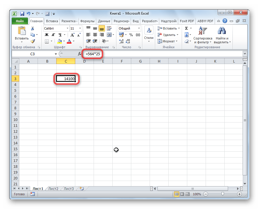
На примере показано умножение 564 на 25. Действие записывается следующей формулой: «=564*25».

Чтобы просмотреть результат вычислений, нужно нажать на клавишу ENTER.
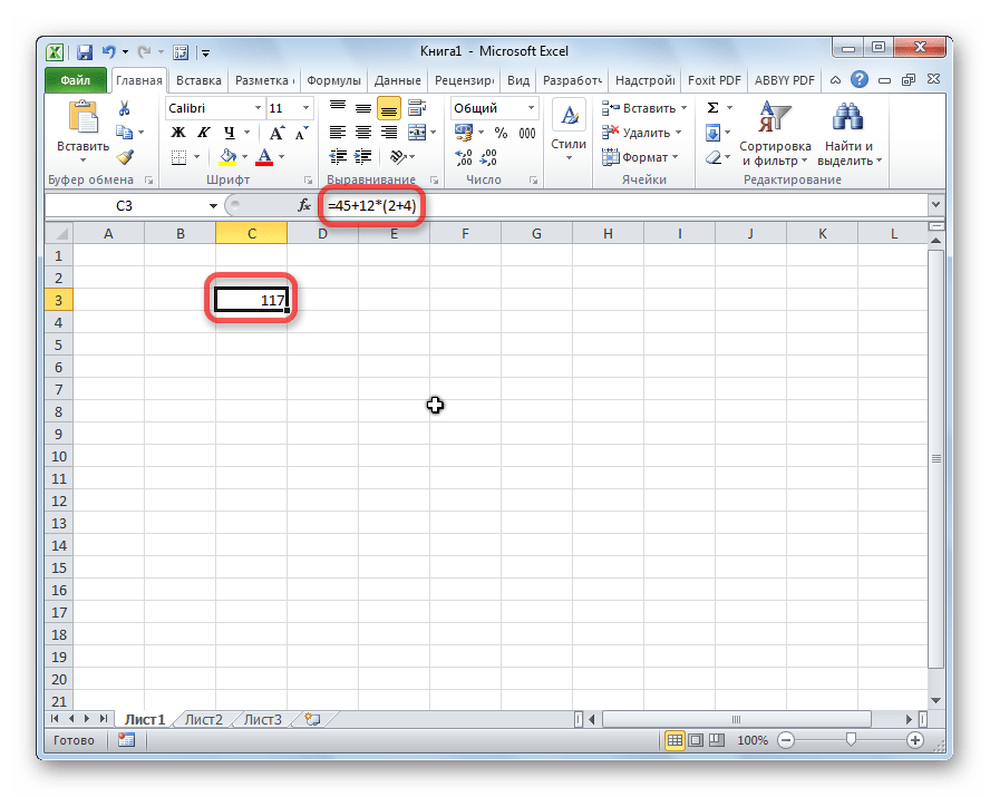
Во время вычислений, нужно помнить, что приоритет арифметических действий в Экселе, такой же, как в обычной математике. Но, знак умножения нужно добавлять в любом случае. Если при записи выражения на бумаге допускается опускать знак умножения перед скобками, то в Excel, для правильного подсчета, он обязателен. Например, выражение 45+12(2+4), в Excel нужно записать следующим образом: «=45+12*(2+4)».
Умножение ячейки на ячейку
Процедура умножения ячейки на ячейку сводится все к тому же принципу, что и процедура умножения числа на число. Прежде всего, нужно определиться, в какой ячейке будет выводиться результат. В ней ставим знак равно (=). Далее, поочередно кликаем по ячейкам, содержание которых нужно перемножить. После выбора каждой ячейки, ставим знак умножения (*).
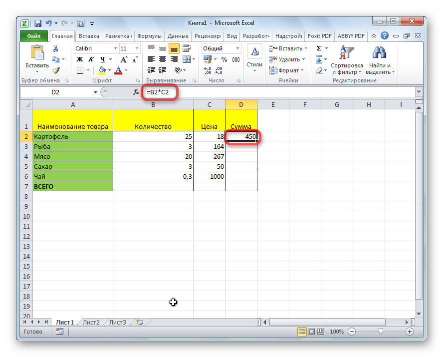
Умножение столбца на столбец
Для того, чтобы умножить столбец на столбец, сразу нужно перемножить самые верхние ячейки этих столбцов, как показано в примере выше. Затем, становимся на нижний левый угол заполненной ячейки. Появляется маркер заполнения. Перетягиваем его вниз с зажатой левой кнопкой мыши. Таким образом, формула умножения копируется во все ячейки столбца.


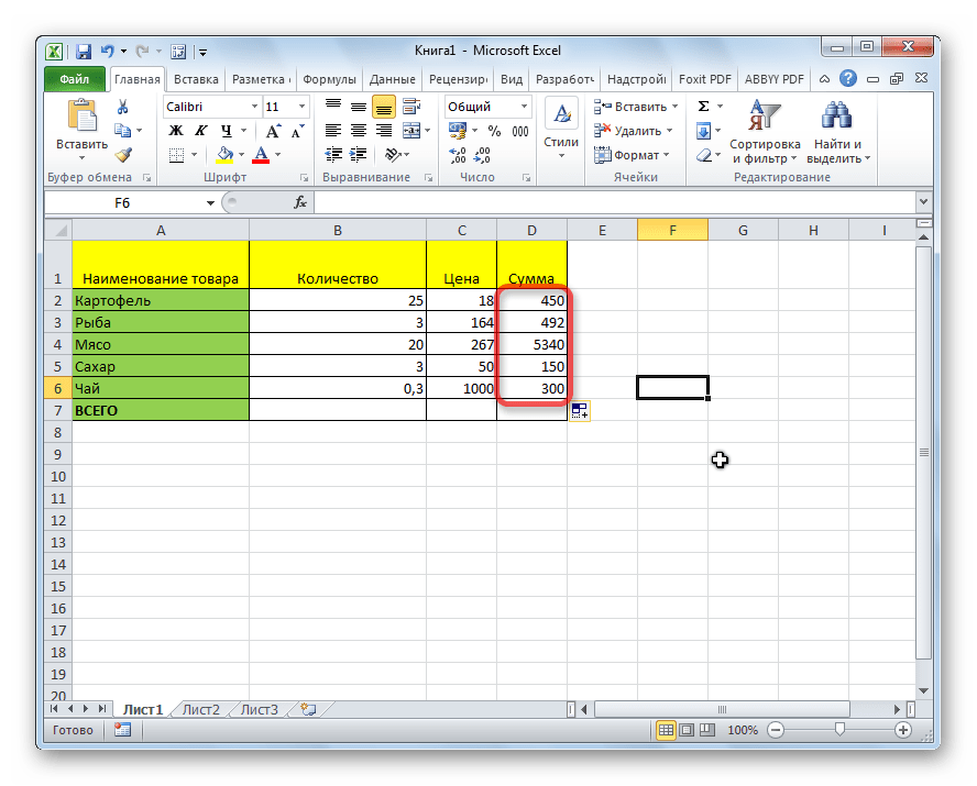
После этого, столбцы будут перемножены.
Аналогично можно множить три и более столбца.
Умножение ячейки на число
Для того, чтобы умножить ячейку на число, как и в выше описанных примерах, прежде всего, ставим знак равно (=) в ту ячейку, в которую вы предполагаете выводить ответ арифметических действий. Далее, нужно записать числовой множитель, поставить знак умножения (*), и кликнуть по ячейке, которую вы хотите умножить.
Для того, чтобы вывести результат на экран, жмем на кнопку ENTER.
Впрочем, можно выполнять действия и в другом порядке: сразу после знака равно, кликнуть по ячейке, которую нужно умножить, а затем, после знака умножения, записать число. Ведь, как известно, от перестановки множителей произведение не меняется.
Таким же образом, можно, при необходимости, умножать сразу несколько ячеек и несколько чисел.
Умножение столбца на число
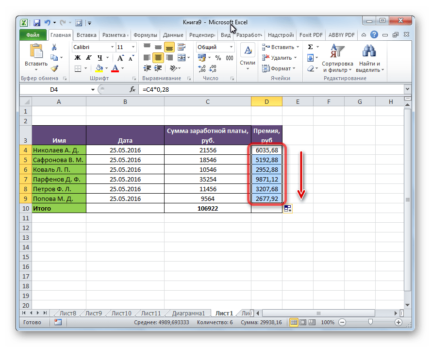
Для того, чтобы умножить столбец на определенное число, нужно сразу умножить на это число ячейку, как это было описано выше. Затем, с помощью маркера заполнения, копируем формулу на нижние ячейки, и получаем результат.
Умножение столбца на ячейку
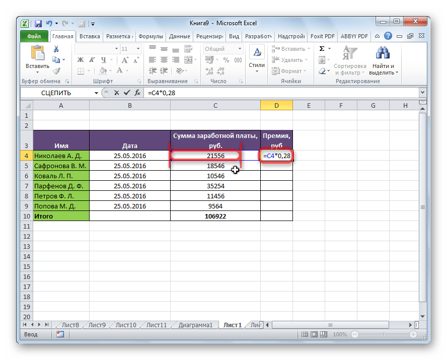
Если в определенной ячейке расположено число, на которое следует перемножить столбец, например, там находится определенный коэффициент, то вышеуказанный способ не подойдет. Это связано с тем, что при копировании будет сдвигаться диапазон обоих множителей, а нам нужно, чтобы один из множителей был постоянным.
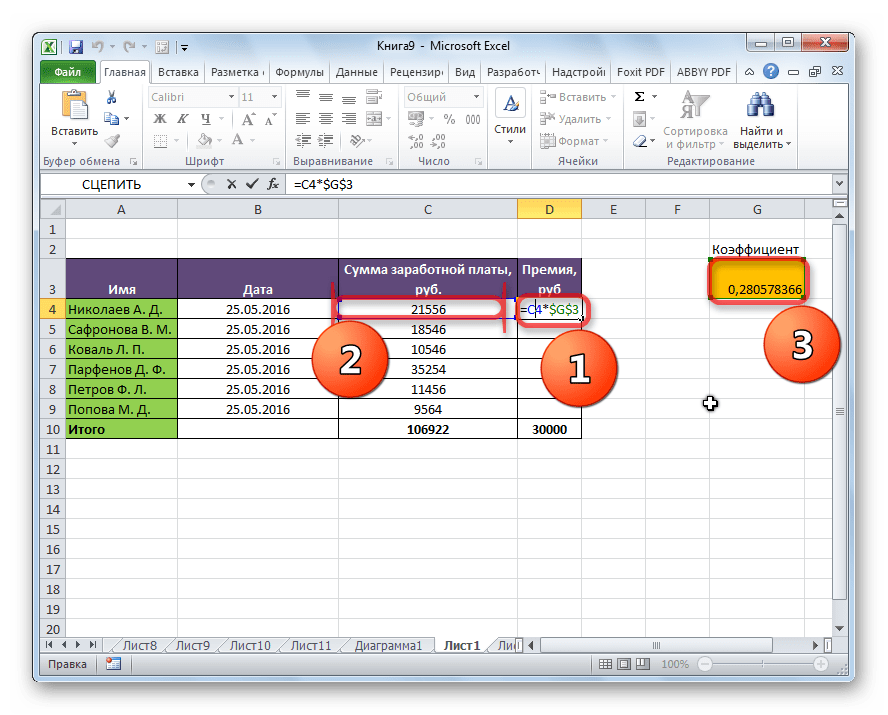
Сначала, умножаем обычным способом первую ячейку столбца на ячейку, в которой содержится коэффициент. Далее, в формуле ставим знак доллара перед координатами столбца и строки ссылки на ячейку с коэффициентом. Таким способом, мы превратили относительную ссылку в абсолютную, координаты которой при копировании изменяться не будут.
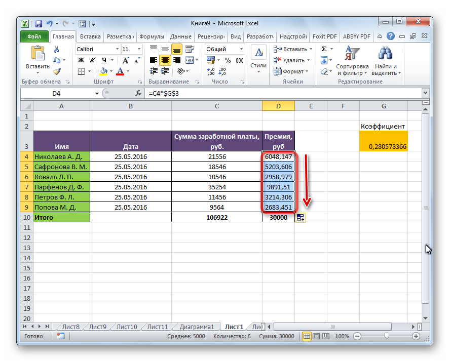
Теперь, осталось обычным способом, с помощью маркера заполнения, скопировать формулу в другие ячейки. Как видим, сразу появляется готовый результат.
Урок: Как сделать абсолютную ссылку
Функция ПРОИЗВЕД
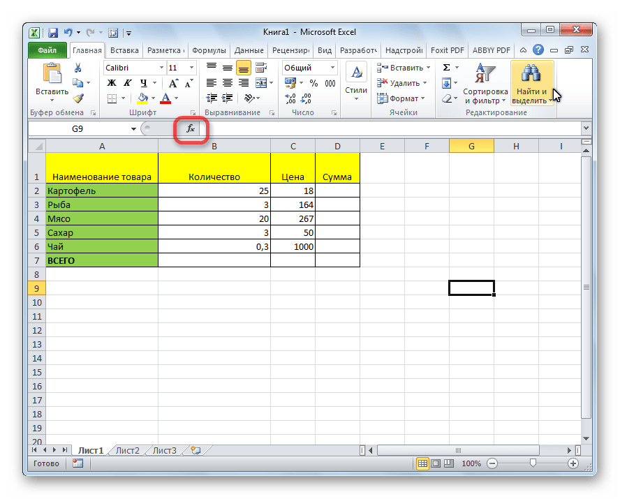
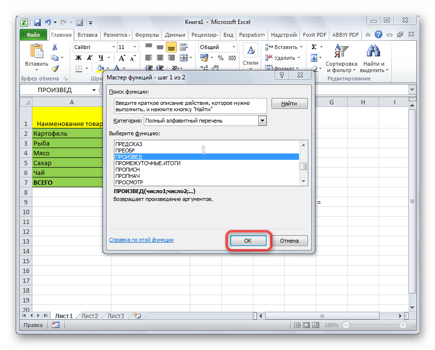
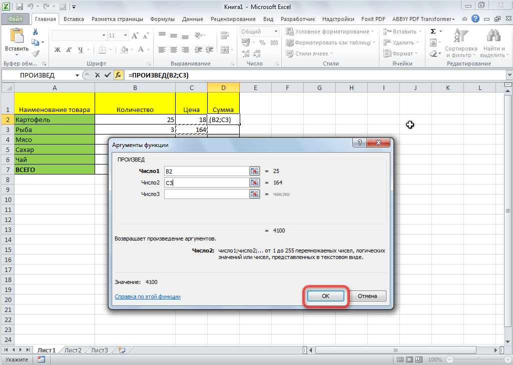
Кроме обычного способа умножения, в программе Excel существует возможность для этих целей использовать специальную функцию ПРОИЗВЕД. Вызвать её можно все теми же способами, что и всякую другую функцию.
- С помощью Мастера функций, который можно запустить, нажав на кнопку «Вставить функцию».
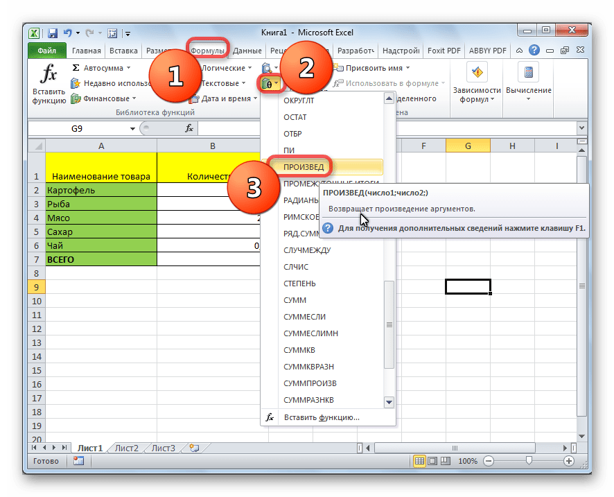
- Через вкладку «Формулы». Находясь в ней, нужно нажать на кнопку «Математические», которая расположена на ленте в блоке инструментов «Библиотека функций». Затем, в появившемся списке следует выбрать пункт «ПРОИЗВЕД».
- Набрать наименование функции ПРОИЗВЕД, и её аргументы, вручную, после знака равно (=) в нужной ячейке, или в строке формул.
Затем, нужно найти функцию ПРОИЗВЕД, в открывшемся окне мастера функций, и нажать кнопку «OK».
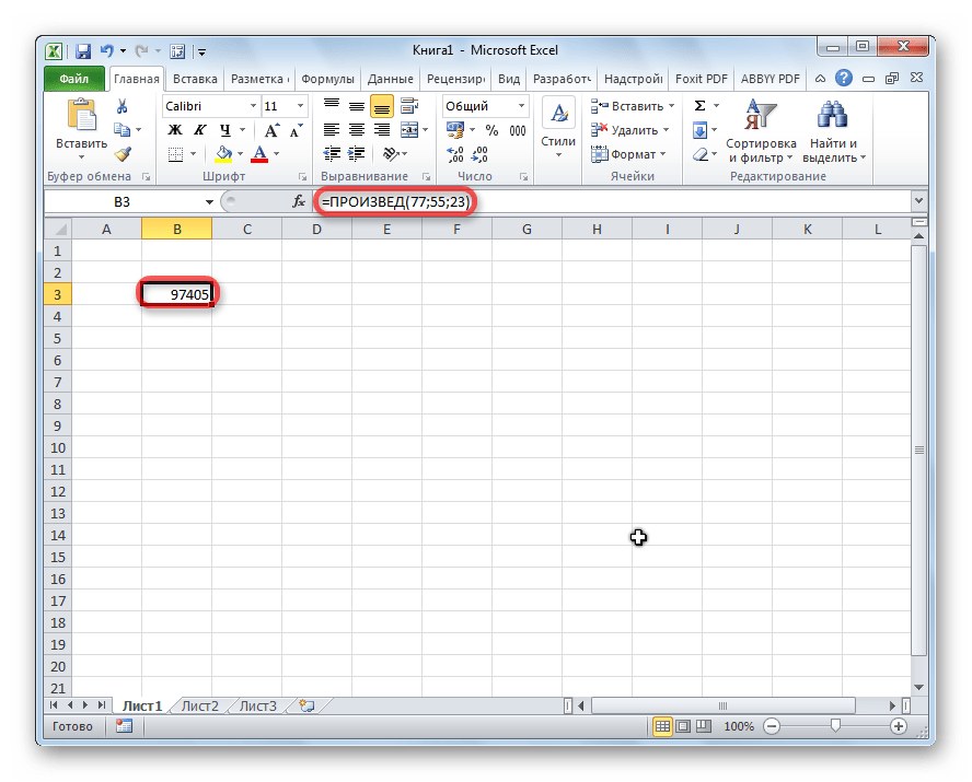
Шаблон функции для ручного ввода следующий: «=ПРОИЗВЕД(число (или ссылка на ячейку); число (или ссылка на ячейку);…)». То есть, если например нам нужно 77 умножить на 55, и умножить на 23, то записываем следующую формулу: «=ПРОИЗВЕД(77;55;23)». Для отображения результата, жмем на кнопку ENTER.
При использовании первых двух вариантов применения функции (с помощью Мастера функций или вкладки «Формулы»), откроется окно аргументов, в которое нужно ввести аргументы в виде чисел, или адресов ячеек. Это можно сделать, просто кликнув по нужным ячейкам. После ввода аргументов, жмем на кнопку «OK», для выполнения вычислений, и вывода результата на экран.
Как видим, в программе Excel существует большое количество вариантов использование такого арифметического действия, как умножение. Главное, знать нюансы применения формул умножения в каждом конкретном случае.
Maintenance Alert: Saturday, April 15th, 7:00pm-9:00pm CT. During this time, the shopping cart and information requests will be unavailable.
Categories: Formulas
Tags: Multiply Formula
While there is no “Excel multiply formula” there are multiple ways to multiply in Excel. For instance, do you use an asterisk (*) to multiply, but hit a brick wall when you apply other arithmetic operators? What about shortcuts for multiplying many numbers in one step?
Read on for three powerful ways to perform an Excel multiply formula.
1. Multiplication with *
To write a formula that multiplies two numbers, use the asterisk (*). To multiply 2 times 8, for example, type “=2*8”.
Use the same format to multiply the numbers in two cells: “=A1*A2” multiplies the values in cells A1 and A2.
You can mix and match the * with other arithmetic operators, such as addition (+), subtraction (-), division (/), and exponentiation (^). In these cases, remember that Excel carries out the operations in the order of PEMDAS: parentheses first, followed by exponents, multiplication, division, addition, and subtraction.
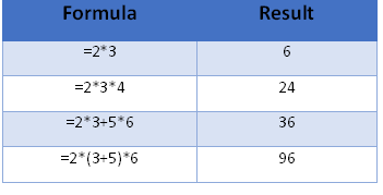
In the following formula “=2*3+5*6,” Excel performs the two multiplication operations first, obtaining 6+30, and add the products to reach 36.
What if you want to add 3+5 before performing the multiplication? Use parentheses. Excel will always evaluate anything in parentheses before resuming the remaining calculations following PEMDAS. In the case of “=3*(3+5)*6”, Excel adds 3 and 5 first, resulting in 8. Then it multiplies 3*8*6 and reaches 144.
If you have trouble remembering the order of PEMDAS, use the Aunt Sally mnemonic device: use the first letters of the sentence, “Please Excuse My Dear Aunt Sally.”
2. Multiplication with the PRODUCT Function
When you need to multiply several numbers, you might appreciate the shortcut formula PRODUCT, which multiplies all of the numbers that you include in the parentheses.
The arguments can be:
- Numbers or formulas separated by commas, such as:
=PRODUCT(3,5+2,8,3.14)
This is equivalent to =3*(5+2)*8*3.14.
- Cell references separated by commas, such as:
=PRODUCT(A3,C3,D3,F3).
This is equivalent to =A3*C3*D3*F3.
- A range of cells containing numbers, or multiple ranges separated by commas, such as:
=PRODUCT(F3:F25),
which is equivalent to =F3*F4*F5*(and so on, all the way up to)*F25, or:
=PRODUCT(F3:F25,H3:H25).
- Any combination of numbers, formulas, cell references, and range references.
In each case, Excel multiplies all the numbers to find the product. If a cell in the range is empty or contains text, Excel leaves that cell’s value out of the calculation. If a cell in the range is zero, the product will be zero.
3. Multiplication of Ranges with the SUMPRODUCT Function
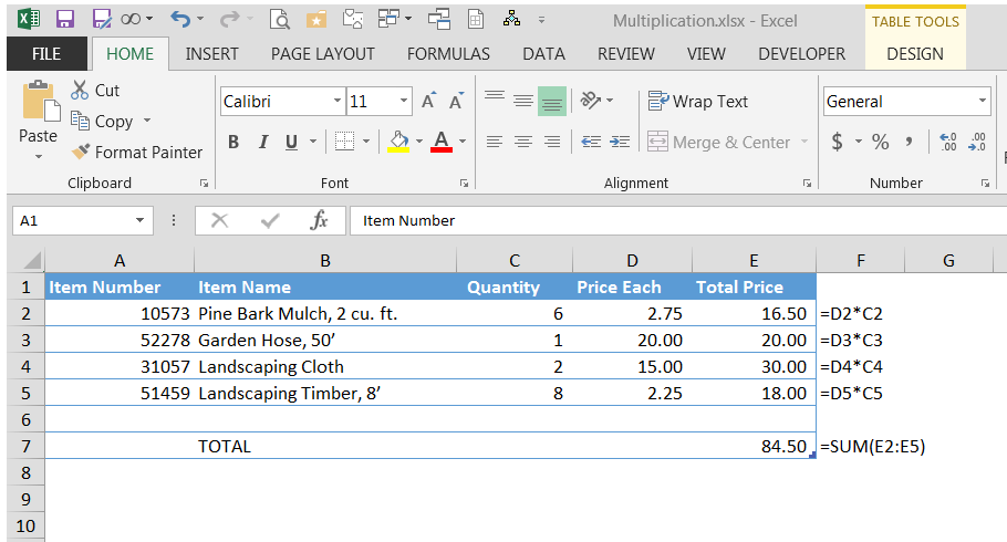
Consider the following invoice. The formula in Column E (with the formula shown to the right of the table) multiplies quantity by the price each to reach an extended price. The total in cell E7 sums up the extended prices.
But what if you don’t want the extended prices to show as separate calculations? What if you want to do it all in one step?
Try the SUMPRODUCT function, which multiplies the cells in two ranges and sums the results.
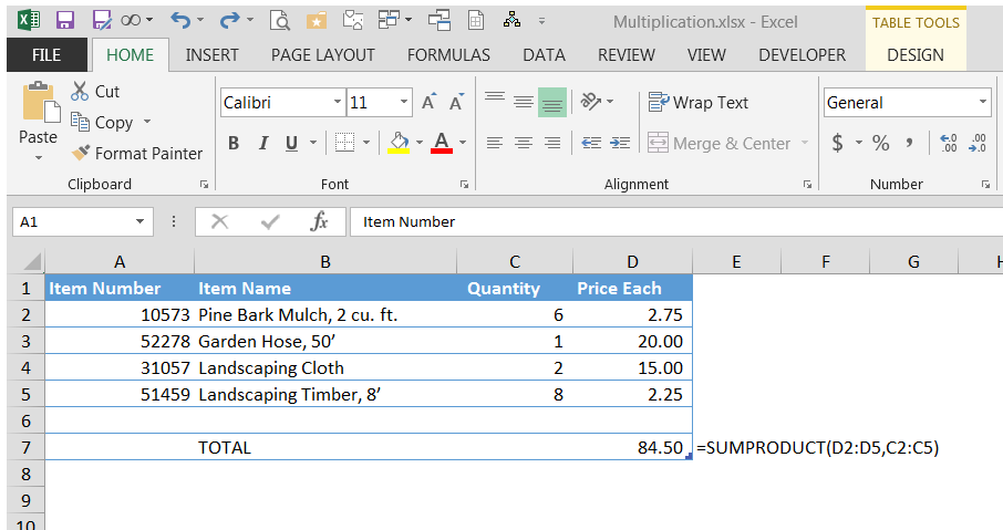
SUMPRODUCT(D2:D5,C2:C5) multiplies D2*C2, D3*C3, etc., and sums the results. Note that the result, 84.50, is the same as the previous example.
This function is invaluable for calculating weighted averages, such as classroom grades or prices based on variable state tax, in which you multiply a range of values by a range containing the weights.
Next Steps
These are but three of the methods to multiply numbers in Excel formulas. When you’ve mastered them, try the PRODUCTIF formula, which multiplies all numbers in a range if a condition is met.
Until then, try mixing and matching the multiplication formulas, using any combination along with other arithmetic functions, to create complex mathematical models.
PRYOR+ 7-DAYS OF FREE TRAINING
Courses in Customer Service, Excel, HR, Leadership,
OSHA and more. No credit card. No commitment. Individuals and teams.