
The best way to learn about Excel 2013 is to start using it. Create a blank workbook and learn the basics of working with columns, cells, and data.
Start using Excel
-
The best way to learn about Excel 2013 is to start using it.
-
You can open an existing workbook, or start with a template. Then, add some data into cells, use the ribbon, use the mini toolbar.
Want more?
What’s new in Excel 2013
Basic tasks in Excel
The best way to learn about Excel 2013 is to start using it.
This is what you see when you start Excel for the first time.
You can open an existing workbook over here or start with a template.
Since this is our first time, let’s keep it simple and select Blank workbook.
The area down here is where you create your worksheet.
And you’ll find all the tools you need to work on it, up here, in this area called the ribbon.
In this area, you’ll find the name box and formula bar.
You’ll see what those do as we go along. Now click somewhere in the work area.
These little rectangles, called cells, each hold one piece of information: some text, a number, or a formula.
Let’s say we want to create a worksheet to track expenses on an expansion project.
Type the first budget item, and press Enter.
There are literally millions of cells in a worksheet, but each one can be identified using this grid system of rows and columns.
For example, the address of this cell is C6; column C, row 6.
The name box shows which cell is selected. You’ll see why addresses are important later. Next, type the other budget items.
This is a breakdown of the work required for the expansion project.
If the text doesn’t fit in the cells, come up here, and hold the mouse over the column border until you see a double-headed arrow.
Then, click and drag the border to widen the column.
Now to make our worksheet more interesting, let’s add rough estimates for each work item in the next column.
To make the numbers look like $ amounts, we’ll add some formatting.
First, select the numbers by clicking the first number and dragging the mouse down the list.
The gray highlighting and green border mean the cells are selected.
Right-click the selection, and the right-click menu opens along with this box up here called the mini-toolbar.
The mini-toolbar changes depending on what you select.
In this case, it contains commands for formatting the cells.
Click the $ sign to format the numbers as $ amounts.
Now it is beginning to look more like a worksheet.
To make it official, let’s add a header row up here, so that anyone who looks at the worksheet will know what the data means in each column.
Next, let’s do something to the data to make it easier to work with.
Select the header and data. Click the top left corner, and drag the mouse to the bottom right.
This time, instead of right-clicking, just hold the mouse over the selection, and a button appears.
Click it and the Quick Analysis lens opens.
This contains a set of tools for helping you analyze your data.
Click TABLES, and then click Table. The data is converted to a table.
You don’t have to do this, but working with data as a table has certain advantages.
For example, you can click these arrows to quickly sort or filter the data.
You also have a lot of commands and options to choose from, up here on the ribbon.
For example, we can add a Total Row to the table or remove the Banded Rows.
While we’re up here, let’s take a closer look at the ribbon.
The commands and options you can work with are organized into these tabs.
Most of the commands, you’ll need are on the HOME tab.
For example, you can come here to format text and numbers, or change a Cell Style.
The INSERT tab has commands for inserting things, like pictures and charts.
We’ll look at some of the other tabs later in the course.
The TABLE TOOLS DESIGN tab is called a contextual tab because it appears only when you are working on the table.
When you select a cell outside the table, the tab goes away.
You’ll also see contextual tabs when you are working with other insertable objects, like Sparklines and Pivot Charts.
Our worksheet is pretty small now, but there’s plenty of room to grow in Excel as your project expands.
However, before we do any more work, let’s save the workbook.
![]()
Download Article
![]()
Download Article
Are you new to Microsoft Excel and need to work on a spreadsheet? Excel is so overrun with useful and complicated features that it might seem impossible for a beginner to learn. But don’t worry—once you learn a few basic tricks, you’ll be entering, manipulating, calculating, and graphing data in no time! This wikiHow tutorial will introduce you to the most important features and functions you’ll need to know when starting out with Excel, from entering and sorting basic data to writing your first formulas.
Things You Should Know
- Use Quick Analysis in Excel to perform quick calculations and create helpful graphs without any prior Excel knowledge.
- Adding your data to a table makes it easy to sort and filter data by your preferred criteria.
- Even if you’re not a math person, you can use basic Excel math functions to add, subtract, find averages and more in seconds.
-

1
Create or open a workbook. When people refer to «Excel files,» they are referring to workbooks, which are files that contain one or more sheets of data on individual tabs. Each tab is called a worksheet or spreadsheet, both of which are used interchangeably. When you open Excel, you’ll be prompted to open or create a workbook.
- To start from scratch, click Blank workbook. Otherwise, you can open an existing workbook or create a new one from one of Excel’s helpful templates, such as those designed for budgeting.
-
2
Explore the worksheet. When you create a new blank workbook, you’ll have a single worksheet called Sheet1 (you’ll see that on the tab at the bottom) that contains a grid for your data. Worksheets are made of individual cells that are organized into columns and rows.
- Columns are vertical and labeled with letters, which appear above each column.
- Rows are horizontal and are labeled by numbers, which you’ll see running along the left side of the worksheet.
- Every cell has an address which contains its column letter and row number. For example, the top-left cell in your worksheet’s address is A1 because it’s in column A, row 1.
- A workbook can have multiple worksheets, all containing different sets of data. Each worksheet in your workbook has a name—you can rename a worksheet by right-clicking its tab and selecting Rename.
- To add another worksheet, just click the + next to the worksheet tab(s).
Advertisement
-
3
Save your workbook. Once you save your workbook once, Excel will automatically save any changes you make by default.[1]
This prevents you from accidentally losing data.- Click the File menu and select Save As.
- Choose a location to save the file, such as on your computer or in OneDrive.
- Type a name for your workbook. All workbooks will automatically inherit the the .XLSX file extension.
- Click Save.


Advertisement
-
1
Click a cell to select it. When you click a cell, it will highlight to indicate that it’s selected.
- When you type something into a cell, the input text is called a value. Entering data into Excel is as simple as typing values into each cell.
- When entering data, the first row of your worksheet (e.g., A1, B1, C1) is typically used as headers for each column. This is helpful when creating graphs or tables which require labels.
- For example, if you’re adding a list of dates in column A, you might click cell A1 and type Date into the cell as the column header.
-
2
Type a word or number into the cell. As you’re typing, you’ll see the letters and/or numbers appear in the cell, as well as in the formula bar at the top of the worksheet.
- When you start practicing more advanced Excel features like creating formulas, this bar will come in handy.
- You can also copy and paste text from other applications into your worksheet, tables from PDFs and the web.
-
3
Press ↵ Enter or ⏎ Return. This enters the data into the cell and moves to the next cell in the column.
-
4
Automatically fill columns based on existing data. Let’s say you want to make a list of consecutive dates or numbers. Or what if you want to fill a column with many of the same values that follow a pattern? As long as Excel can recognize some sort of pattern in your data, such as a particular order, you can use Autofill to automatically populate data into the rest of your column. Here’s a trick to see it in action.
- In a blank column, type 1 into the first cell, 2 into the second cell, and then 3 into the third cell.
- Hover your mouse cursor over the bottom-right corner of the last cell in your series—it will turn to a crosshair.
- Click and drag the crosshair down the column, then release the mouse button once you’ve gone down as far as you like. By default, this will fill the remaining cells with the value of the selected cell—at this point, you’ll probably have something like 1, 2, 3, 3, 3, 3, 3, 3.
- Click the small icon at the bottom-right corner of the filled data to open AutoFill options, and select Fill Series to automatically detect the series or pattern. Now you’ll have a list of consecutive numbers. Try this cool feature out with different patterns!
- Once you get the hang of AutoFill, you’ll have to try flash fill, which you can use to join two columns of data into a single merged column.
-
5
Adjust the column sizes so you can see all of the values. Sometimes typing long values into a cell hides the value and displays hash symbols ### instead of what you’ve typed. If you want to be able to see everything, you can snap the cell contents to the width of the widest cell. For example, let’s say we have some long values in column B:
- To expand the contents of column B, hover the cursor over the dividing line between the B and C at the top of the worksheet—once your cursor is right on the line, it will turn to two arrows pointing in either direction.[2]
- Click and drag the separator until the column is wide enough to accommodate your data, or just double-click the separator to instantly snap the column to the size of the widest value.
- To expand the contents of column B, hover the cursor over the dividing line between the B and C at the top of the worksheet—once your cursor is right on the line, it will turn to two arrows pointing in either direction.[2]
-
6
Wrap text in a cell. If your longer values are now awkwardly long, you can enable text wrapping in one or more cells. Just click a cell (or drag the mouse to select multiple cells), click the Home tab, and then click Wrap Text on the toolbar.
-
7
Edit a cell value. If you need to make a change to a cell, you can double-click the cell to activate the cursor, and then make any changes you need. When you’re finished, just press Enter or Return again.
- To delete the contents of a cell, click the cell once and press delete on your keyboard.
-
8
Apply styles to your data. Whether you want to highlight certain values with color so they stand out or just want to make your data look pretty, changing the colors of cells and their containing values is easy—especially if you’re used to Microsoft Word:
- Select a cell, column, row, or multiple cells at once.
- On the Home tab, click Cell Styles if you’d like to quickly apply quick color styles.
- If you’d rather use more custom options, right-click the selected cell(s) and select Format Cells. Then, use the colors on the Fill tab to customize the cell’s background, or the colors on the Font tab for value colors.
-
9
Apply number formatting to cells containing numbers. If you have data that contains numbers such as prices, measurements, dates, or times, you can apply number formatting to the data so it will display consistently.[3]
By default, the number format is General, which means numbers display exactly as you type them.- Select the cell you want to format. If you’re working with an entire column or row, you can just click the column letter or row number to select the whole thing.
- On the Home tab, click the drop-down menu at the top-center—it’ll say General by default, unless you selected cells that Excel recognizes as a different type of number like Currency or Time.
- Choose one of the formatting options in the list, such as Short Date or Percentage, or click More Number Formats at the bottom to expand all options (we recommend this!).
- If you selected More Number Formats, the Format Cells dialog will expand to the Number tab, where you’ll see several categories for number types.
- Select a category, such as Currency if working with money, or Date if working with dates. Then, choose your preferences, such as a currency symbol and/or decimal places.
- Click OK to apply your formatting.


Advertisement
-
1
Select all of the data you’ve entered so far. Adding your data to a table is the easiest way to work with and analyze data.[4]
Start by highlighting the values you’ve entered so far, including your column headers. Tables also make it easy to sort and filter your data based on values.- Tables traditionally apply different or alternating colors to every other row for easy viewing. Many table options also add borders between cells and/or columns and rows.
-
2
Click Format as Table. You’ll see this at the top-center part of the Home tab.[5]
-
3
Select a table style. Choose any of Excel’s default table styles to get started. You’ll see a small window titled «Create Table» once selected.
- Once you get the hang of tables, you can return here to customize your table further by selecting New Table Style.
-
4
Make sure «My table has headers» is selected and click OK. This tells Excel to turn your column headers into drop-down menus that you can easily sort and filter. Once you click OK, you’ll see that your data now has a color scheme and drop-down menus.
-
5
Click the drop-down menu at the top of a column. Now you’ll see options for sorting that column, as well as several options for filtering all of your data based on its values.
-
6
Choose which data to display based on values in this column. The simplest way to do this is to uncheck the values you don’t want to display—if you uncheck a particular date, for example, you’ll prevent rows that contain the selected date in from appearing in your data. You can also use Text Filters or Number Filters, depending on the type of data in the column:
- If you chose a numerical column, select Number Filters, then choose an option like Greater Than… or Does Not Equal to be extra specific about which values to hide.
- For text columns, you can choose Text Filters, where you can specify things like Begins with or Contains.
- You can also filter by cell color.
-
7
Click OK. Your data is now filtered based on your selections. You’ll also see a small funnel icon in the drop-down menu, which indicates that the data is filtering out certain values.
- To unfilter your data, click the funnel icon, click Clear filter from (column name), and then click OK.
- You can also filter columns that aren’t in tables. Just select a column and click Filter on the Data tab to add a drop-down to that column.
-
8
Sort your data in ascending or descending order. Click the drop-down arrow at the top of a column to view sorting options—these allow you to sort all of your data in order based on the current column.
- If you’re working with numbers, click Smallest to Largest to sort in ascending order, or Largest to Smallest for descending order.[6]
- If you’re working with text values, Sort A to Z will sort in ascending order, while Sort Z to A will sort in reverse.
- When it comes to sorting dates and times, Sort Oldest to Newest will sort with the earliest date at the top and the oldest date at the bottom, and Newest to Oldest displays the dates in descending order.
- When you sort a column, all other columns in the table adjust based on the sort.
- If you’re working with numbers, click Smallest to Largest to sort in ascending order, or Largest to Smallest for descending order.[6]


Advertisement
-
1
Select the data in your worksheet. Excel’s Quick Analysis feature is the easiest way to perform basic calculations (including totals, averages, and counts) and create meaningful tables or graphs without the need for advanced Excel knowledge.[7]
Use your mouse to select your data (including your column headers) to get started. -
2
Click the Quick Analysis icon. This is the small icon that pops up at the bottom-right corner of your selection. It looks like a window with some colored lines.
-
3
Select an analysis type. You’ll see several tabs running along the top of the window, each of which gives you different option for visualizing your data:
- For math calculations, click the Totals tab, where you can select Sum, Average, Count, %Total, or Running Total. You’ll be able to choose whether to display the results at the bottom of each column or to the right.
- To create a chart, click the Charts tab, then select a chart to visualize your data. Before you settle on a chart, just hover the cursor over each option to see a preview.
- To add quick chart data to individual cells, click the Sparklines tab and choose a format. Again, you can hover the cursor over each option to see a preview.
- To instantly apply conditional formatting (which is usually a little more complex in Excel) based on your data, use the Formatting tab. Here you can choose an option like Color or Data Bars, which apply colors to your data based on trends.


Advertisement
-
1
Quickly add data with AutoSum. AutoSum is a built-in Excel function that makes it easy to find the total of one or more columns in a few clicks. Functions or formulas that perform calculations and other tasks based on the values of cells. When you use a function to get something done, you’re creating a formula, which is like a math equation. If you have a column or row of numbers you want to add:
- Click the cell below the numbers you want to add (if a column) or to the right (if a row).[8]
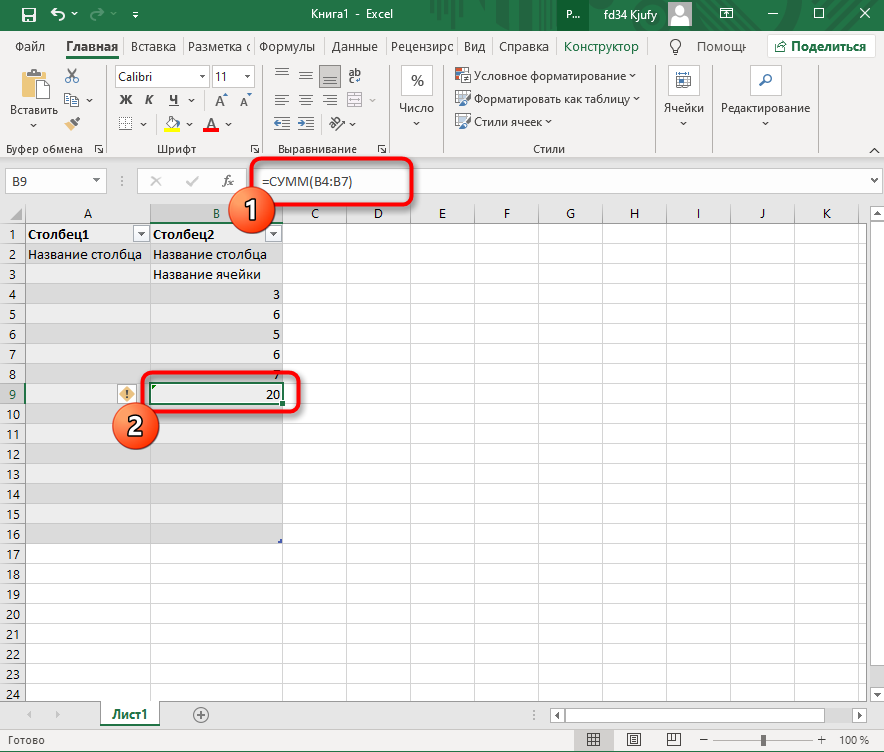
- On the Home tab, click AutoSum toward the upper-right corner of the app. A formula beginning with =SUM(cell+cell) will appear in the field, and a dotted line will surround the numbers you’re adding.
- Press Enter or Return. You should now see the total of the numbers in the selected field. This is here because you created your first formula—which you didn’t have to write by hand!
- If you change any numbers in your data after using AutoSum, the AutoSum value will update automatically.
- Click the cell below the numbers you want to add (if a column) or to the right (if a row).[8]
-
2
Write a simple math formula. AutoSum is just the beginning—Excel is famous for its ability to do all sorts of simple and complex math calculations on data. Fortunately, you don’t have to be a math whiz to create simple formulas to create everyday math formulas, like adding, subtracting, and multiplying. Here’s some basic formulas to get you started:
-
Add: — Type =SUM(cell+cell) (e.g.,
=SUM(A3+B3)) to add two cells’ values together, or type =SUM(cell,cell,cell) (e.g.,=SUM(A2,B2,C2)) to add a series of cell values together.- If you want to add all of the numbers in a whole column (or in a section of a column), type =SUM(cell:cell) (e.g.,
=SUM(A1:A12)) into the cell you want to use to display the result.
- If you want to add all of the numbers in a whole column (or in a section of a column), type =SUM(cell:cell) (e.g.,
-
Subtract: Type =SUM(cell-cell) (e.g.,
=SUM(A3-B3)) to subtract one cell value from another cell’s value. -
Divide: Type =SUM(cell/cell) (e.g.,
=SUM(A6/C5)) to divide one cell’s value by another cell’s value. -
Multiply: Type =SUM(cell*cell) (e.g.,
=SUM(A2*A7)) to multiply two cell values together.
-
Add: — Type =SUM(cell+cell) (e.g.,


Advertisement
-
1
Select a cell for an advanced formula. What if you need to do something more complicated than just adding numbers? Even if you don’t know how to write formulas by hand, you can still create useful formulas that work with your data in various ways. Start by clicking the cell in which you want to display your formula.
-
2
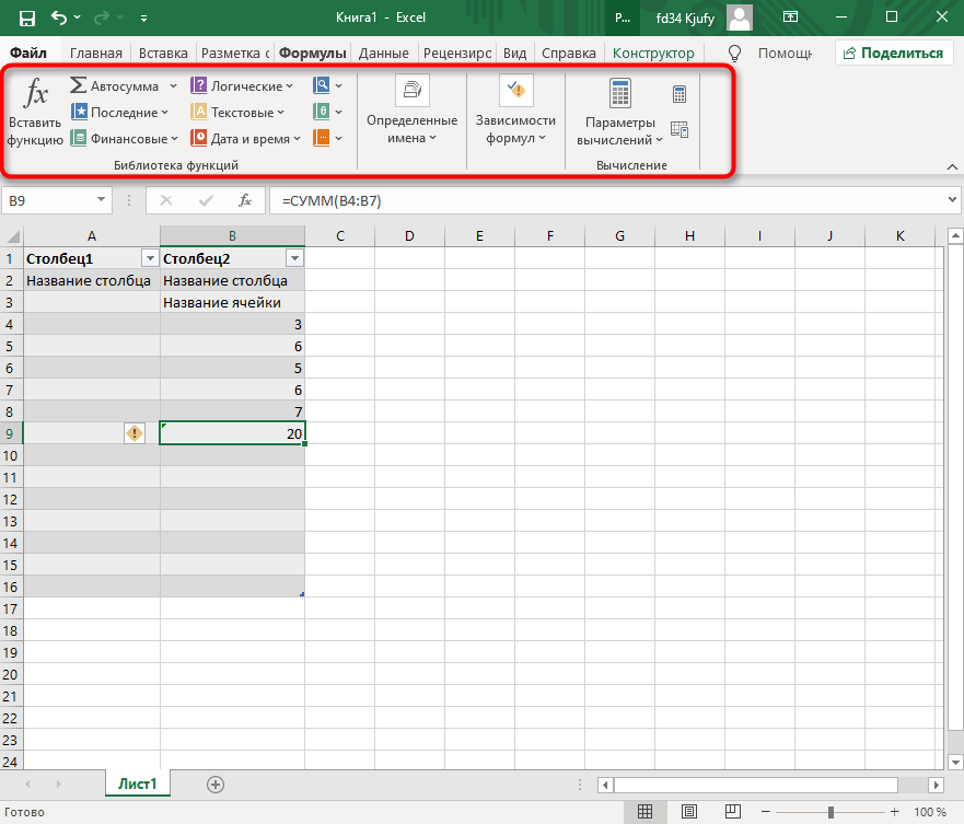
Click the Formulas tab. It’s a tab at the top of the Excel window.
-
3
Explore the Function Library. Several function categories appear in the toolbar, such as Financial, Text, and Math & Trig. Click the options to check out the types of functions available, though they might not make a whole lot of sense just yet.
-
4
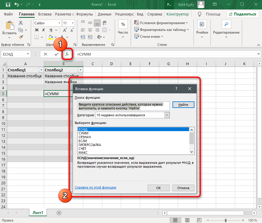
Click Insert Function. This option is in the far-left side of the Formulas toolbar. This opens the Insert Function window, which gives you a more detailed breakdown of each function.
-
5
Click a function to learn about it. You can type what you want to do (such as round), or choose a category to filter the list of functions. Then, click any function to read a description of how it works and view its syntax.
- For example, to select the formula for finding the tangent of an angle, you would scroll down and click the TAN option.
-
6
Select a function and click OK. This creates a formula based on the selected function.
-
7
Fill out the function’s formula. When prompted, type in the number or select a cell for which you want to use the formula.
- For example, if you select the TAN function, you’ll type in the number for which you want to find the tangent, or select the cell that contains that number.
- Depending on your selected function, you may need to click through a couple of on-screen prompts.
-
8
Press ↵ Enter or ⏎ Return to run the formula. Doing so applies your function and displays it in your selected cell.


Advertisement
-
1
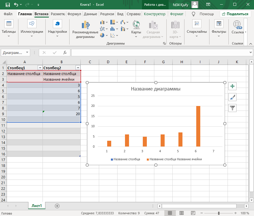
Set up the chart’s data. If you’re creating a line graph or a bar graph, for example, you’ll want to use one column of cells for the horizontal axis and one column of cells for the vertical axis. The best way to do this is to place your data in a table.
- Typically speaking, the left column is used for the horizontal axis and the column immediately to the right of it represents the vertical axis.
-
2
Select the data in your table. Click and drag your mouse from the top-left cell of the data down to the bottom-right cell of the data.
-
3
Click the Insert tab. It’s a tab at the top of the Excel window.
-
4
Click Recommended Charts. You’ll find this option in the «Charts» section of the Insert toolbar. A window with different chart templates will appear.
-
5
Select a chart template. Click the chart template you want to use based on the type of data you’re working with. If you don’t see a chart type you like, click the All Charts tab to explore by category, such as Pie, Bar, and X Y Scatter.
-
6
Click OK. It’s at the bottom of the window. This creates your chart.
-
7
Use the Chart Design tab to customize your chart. Any time you click your chart, the Chart Design tab will appear at the top of Excel. You can adjust the chart style here, change colors, and add additional elements.
-
8
Double-click a chart element to manage it in the Format panel. When you double-click something on your chart, such as a value, line, or bar, you’ll see options you can edit in the panel on the right side of excel. Here you can change the axis labels, alignment, and legend data.


Advertisement
Add New Question
-
Question
How do you add a check mark or an X mark to a cell?

You can go into Insert, then Symbol, and choose the symbol you want. After that, you can just copy and paste the symbol from one cell to another.
-
Question
Can I add work sheets on Excel?
Yes. At the bottom left of the Excel you will see the list of sheets. To the left of those sheets you will find a «+» sign. Click on it.
-
Question
How do I move cell contents to another cell?
Highlight the cell, right-click, and click Copy. Click destination cell, right-click and Paste.
See more answers
Ask a Question
200 characters left
Include your email address to get a message when this question is answered.
Submit
Advertisement
Video
Thanks for submitting a tip for review!
References
About This Article
Article SummaryX
1. Purchase and install Microsoft Office.
2. Enter data into individual cells.
3. Format cells based on certain criteria.
4. Organize data into rows and columns.
5. Perform math operations using formulas.
6. Use the Formulas tab to find additional formulas.
7. Use data to create charts.
8. Import data from other sources.
Did this summary help you?
Thanks to all authors for creating a page that has been read 646,263 times.
Reader Success Stories
-

«I am applying for a job that requires comprehensive knowledge of Excel. Well, I don’t have it, but this article…» more
Is this article up to date?
How To Use Excel:
A Beginner’s Guide To Getting Started
Written by co-founder Kasper Langmann, Microsoft Office Specialist.
Excel is a powerful application—but it can also be very intimidating.
That’s why we’ve put together this beginner’s guide to getting started with Excel.
It will take you from the very beginning (opening a spreadsheet), through entering and working with data, and finish with saving and sharing.
It’s everything you need to know to get started with Excel.
If you want to tag along as you read, please download the free sample Excel workbook here.
Opening an Excel spreadsheet
When you first open Excel (by double-clicking the icon or selecting it from the Start menu), the application will ask what you want to do.

If you want to open a new Excel spreadsheet, click Blank workbook.
To open an existing spreadsheet (like the example workbook you just downloaded), click Open Other Workbooks in the lower-left corner, then click Browse on the left side of the resulting window.

Then use the file explorer to find the Excel workbook you’re looking for, select it, and click Open.
Workbooks vs. spreadsheets
There’s something we should clear up before we move on.
A workbook is an Excel file. It usually has a file extension of .XLSX (if you’re using an older version of Excel, it could be .XLS).
A spreadsheet is a single sheet inside a workbook. There can be many sheets inside of a workbook, and they’re accessed via the tabs at the bottom of the screen.
A spreadsheet (a.k.a. a sheet/tab) contains all the cells you can see and use in the >1 million rows >16,000 columns.
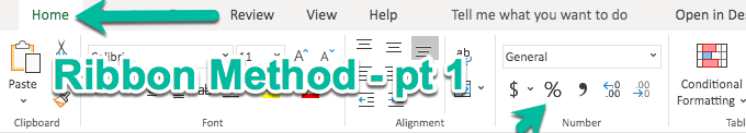
Working with the Ribbon
The Ribbon is the central control panel of Excel. You can do just about everything you need to directly from the Ribbon.
Where is this powerful tool? At the top of the window:

There are a number of tabs, including the File tab, Home tab, Insert tab, Data tab, Review tab, and a few others. Each tab contains different buttons.
Try clicking on a few different tabs to see which buttons appear below them.
 Kasper Langmann, Co-founder of Spreadsheeto
There’s also a very useful search bar in the Ribbon. It says Tell me what you want to do. Just type in what you’re looking for, and Excel will help you find it.

Most of the time, you’ll be in the Home tab of the Ribbon. But Formulas and Data are also very useful (we’ll be talking about formulas shortly).
Pro tip: Ribbon sections
In addition to tabs, the Ribbon also has some smaller sections. And when you’re looking for something specific, those sections can help you find it.
For example, if you’re looking for sorting and filtering options, you don’t want to hover over dozens of buttons finding out what they do.
Instead, skim through the section names until you find what you’re looking for:

Managing your sheets
As we saw, workbooks can contain multiple sheets.
You can manage those sheets with the sheet tabs near the bottom of the screen. Click a tab to open that particular worksheet.
If you’re using our example workbook, you’ll see two sheets, called Welcome and Thank You:

To add a new worksheet, click the + (plus) button at the end of the list of sheets.
You can also reorder the sheets in your workbook by dragging them to a new location.
And if you right-click a worksheet tab, you’ll get a number of options:

For now, don’t worry too much about these options. Rename and Delete are useful, but the rest needn’t concern you.
Kasper Langmann, Co-founder of SpreadsheetoEntering data
Now it’s time to enter some data!
And while entering data is one of the most central and important things you can do in Excel, it’s almost effortless.
Just click into a blank cell and start typing.
Go ahead, try it! Type your name, birthday, and your favorite number into some blank cells.
Kasper Langmann, Co-founder of SpreadsheetoYou can also copy (Ctrl + C), cut (Ctrl + X), and paste (Ctrl + V) any data you’d like (or read our full guide on copying and pasting here).
Try copying and pasting the data from multiple cells inthe example spreadsheet into another column.
You can also copy data from other programs into Excel.
Try copying this list of numbers and pasting it into your sheet:
- 17
- 24
- 9
- 00
- 3
- 12
That’s all we’re going to cover for basic data entry. Just know that there are lots of other ways to get data into your spreadsheets if you need them.
Kasper Langmann, Co-founder of SpreadsheetoBasic calculations
Now that we’ve seen how to get some basic data into our spreadsheet, we’re going to do some things with it.
Running basic calculations in Excel is easy. First, we’ll look at how to add two numbers.
Important: start calculations with = (equals)
When you’re running a calculation (or a formula, which we’ll discuss next), the first thing you need to type is an equals sign. This tells Excel to get ready to run some sort of calculation.
So when you see something like =MEDIAN(A2:A51), make sure you type it exactly as it is—including the equals sign.
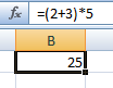
Let’s add 3 and 4. Type the following formula in a blank cell:
=3+4
Then hit Enter.

When you hit Enter, Excel evaluates your equation and displays the result, 7.
But if you look above at the formula bar, you’ll still see the original formula.
That’s a useful thing to keep in mind, in case you forget what you typed originally.
You can also edit a cell in the formula bar. Click on any cell, then click into the formula bar and start typing.
Kasper Langmann, Co-founder of SpreadsheetoPerforming subtraction, multiplication, and division is just as easy. Try these formulas:
- =4-6
- =2*5
- =-10/3
What we’re going to cover next is one of the most important things in Excel. We’re giving it a very basic overview here, but feel free to read our post on cell references to get the details.
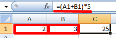
Kasper Langmann, Co-founder of SpreadsheetoNow let’s try something different. Open up the first sheet in the example workbook, click into cell C1, and type the following:
=A1+B1
Hit Enter.
You should get 82, the sum of the numbers in cells A1 and B1.
Now, change one of the numbers in A1 or B1 and watch what happens:
Because you’re adding A1 and B1, Excel automatically updates the total when you change the values in one of those cells.
Try doing different types of arithmetic on the other numbers in columns A and B using this method.
Unlocking the power of functions
Excel’s greatest power lies in functions. These let you run complex calculations with a few keypresses.
We’ll barely scratch the surface of functions here. Check out our other blog posts to see some of the great things you can do with functions!
Kasper Langmann, Co-founder of SpreadsheetoMany formulas take sets of numbers and give you information about them.
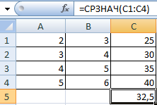
For example, the AVERAGE function gives you the average of a set of numbers. Let’s try using it.
Click into an empty cell and type the following formula:
=AVERAGE(A1:A4)
Then hit Enter.

The resulting number, 0.25, is the average of the numbers in cells A1, A2, A3, and A4.
Cell range notation
In the formula above, we used “A1:A4” to tell Excel to look at all the cells between A1 and A4, including both of those cells. You can read it as “A1 through A4.”
You can also use this to include numbers in different columns. “A5:C7” includes A5, A6, A7, B5, B6, B7, C5, C6, and C7.
There are also functions that work on text.
Let’s try the CONCATENATE function!
Click into cell C5 and type this formula:
=CONCATENATE(A5, ” “, B5)
Then hit Enter.
You’ll see the message “Welcome to Spreadsheeto” in the cell.
How did this happen? CONCATENATE takes cells with text in them and puts them together.
We put the contents of A5 and B5 together. But because we also needed a space between “to” and “Spreadsheeto,” we included a third argument: the space between two quotes.
Remember that you can mix cell references (like “A5″) and typed values (like ” “) in formulas.
Kasper Langmann, Co-founder of SpreadsheetoExcel has dozens of useful functions. To find the function that will solve a particular problem, head to the Formulas tab and click on one of the icons:

Scroll through the list of available functions, and select the one you want (you may have to look around for a while).
Then Excel will help you get the right numbers in the right places:

If you start typing a formula, starting with the equals sign, Excel will help you by showing you some possible functions that you might be looking for:

And finally, once you’ve typed the name of a formula and the opening parenthesis, Excel will tell you which arguments need to go where:

If you’ve never used a function before, it might be difficult to interpret Excel’s reminders. But once you get more experience, it’ll become clear.
This is a tiny preview of how functions work and what they can do. It should be enough to get you going on the tasks you need to accomplish right away.
Kasper Langmann, Co-founder of SpreadsheetoSaving and sharing your work
After you’ve done a bunch of work with your spreadsheet, you’re going to want to save your changes.
Hit Ctrl + S to save. If you haven’t yet saved your spreadsheet, you’ll be asked where you want to save it and what you want to call it.
You can also click the Save button in the Quick Access Toolbar:

It’s a good idea to get into the habit of saving often. Trying to recover unsaved changes is a pain!
Kasper Langmann, Co-founder of SpreadsheetoThe easiest way to share your spreadsheets is via OneDrive.
Click the Share button in the top-right corner of the window, and Excel will walk you through sharing your document.

You can also save your document and email it, or use any other cloud service to share it with others.
That’s it – Now what?
This was how to use Excel.
Or… at least a small fraction of it.
Microsoft Excel can be intimidating, but once you get the basics down, it’s easier to learn the more advanced functions.
This was your introduction to “the basics”. So, if you’re not ready to get some advanced Excel knowledge, go ahead and practice with some of the existing data at the office 🧑🏼💻
If you’re ready to take your next steps, go ahead and enroll in my 30-minute free online course where you learn: IF, SUMIF, VLOOKUP, and data cleaning.
These are some of the most important topics of Excel💪🏼
Other resources
Now, you can’t excel at Excel without mastering some of the lookup functions like VLOOKUP and the new XLOOKUP.
But also, you don’t wanna miss out on pivot tables. You can use these to transform your Microsoft Excel data into insightful reports in just a few clicks🤯
Or if you’re into automating Excel spreadsheet formatting, go ahead and read my guide to conditional formatting here.
Kasper Langmann2023-02-23T14:45:07+00:00
Page load link
Если текстовым редактором Word с грехом пополам владеет большая часть пользователей компьютеров, то с не менее знаменитым табличным процессором дела обстоят не столь радужно. Многие просто не видят, каким образом можно использовать эту программу для повседневных нужд, пока не столкнутся с необходимостью выполнять расчёты на больших выборках данных.
Но и здесь имеются проблемы: не поняв без посторонней помощи принципы работы Excel, пользователи бросают это занятие и больше к нему не возвращаются.

Сегодняшняя статься предназначена для обеих категорий населения: простые пошаговые инструкции позволят начать практическое освоение программы. Ведь, на самом деле, Excel позволяет не только выполнять расчёты в табличном представлении – приложение можно использовать для составления диаграмм, многофакторных графиков, подробных отчётов.
Да, таблицы в Word и Excel – это совершенно разные вещи, но на самом деле работать с табличными данными вовсе не сложно. И для этого совсем не обязательно быть программистом.
Начало работы
Практика – лучший способ получить базовые навыки в любой профессии. Табличный процессор от Microsoft не является исключением. Это весьма полезное приложение, применимое в самых разных областях деятельности, позволяющее организовать быстрые вычисления вне зависимости от количества исходных данных.
Освоив Excel, вы вряд ли станете экспертом по реляционным базам данных, но полученных навыков окажется вполне достаточно для получения статуса «уверенный пользователь». А это не только моральное удовлетворение и способ похвастаться перед друзьями, но и небольшой плюсик к вашему резюме.

Итак, для начала давайте ознакомимся с основными терминами, касающимися Excel:
- таблица – это двумерное представление наборов чисел или иных значений, размещённых в строках и столбцах. Нумерация строк – числовая, от 1 и далее до бесконечности. Для столбцов принято использовать буквы латинского алфавита, причём, если нужно больше 26 столбцов, то после Z будут идти индексы АА, АВ и так далее;
- таким образом, каждая ячейка, расположенная на пересечении столбца и строки, будет иметь уникальный адрес типа А1 или С10. Когда мы будем работать с табличными данными, обращение к ячейкам будет производиться по их адресам, вернее – по диапазонам адресов (например, А1:А65, разделителем здесь является двоеточие). В Excel табличный курсор привязывается не к отдельным символам, а к ячейке в целом – это упрощает манипулирование данными. Это означает, что с помощью курсора вы можете перемещаться по таблице, но не внутри ячейки – для этого имеются другие инструменты;
- под рабочим листом в Excel понимают конкретную таблицу с набором данных и формулами для вычислений;
- рабочая книга – это файл с расширением xls, в котором может содержаться один или несколько рабочих листов, то есть это может быть набор связанных таблиц;
- работать можно не только с отдельными ячейками или диапазонами, но и с их совокупностью. Отдельные элементы списка разделяются точкой с запятой (В2;В5:В12);
- с помощью такой индексации можно выделять отдельные строки, столбцы или прямоугольные области;
- с объектами таблицы можно производить различные манипуляции (копирование, перемещение, форматирование, удаление).

Как работать в программе Excel: пособие для начинающих
Итак, мы получили некий минимум теоретических сведений, позволяющих приступить к практической части. А теперь рассмотрим, как работать в Excel. Разумеется, после запуска программы нам нужно создать таблицу. Сделать это можно разными способами, выбор которых осуществляется с учётом ваших предпочтений и стоящих перед вами задач.
Изначально мы имеем пустую таблицу, но уже разбитую на ячейки, с пронумерованными строками и столбцами. Если распечатать такую таблицу, получим чистый лист, без рамок и границ.
Давайте разберёмся, как работать с элементами таблицы – стройками, столбцами и отдельными ячейками.

Как выделить столбец/строку
Для выделения столбца необходимо щёлкнуть кнопкой мыши по его наименованию, представленному латинской буквой или комбинацией букв.
Соответственно, для выделения строки нужно щелкнуть мышкой по цифре, соотносящейся с нужной строкой.
Для выделения диапазона строк или столбцов действуем следующим образом:
- щёлкаем правой кнопкой по первому индексу (буква или цифра), при этом строка/столбец выделится;
- отпускаем кнопку и ставим курсор на второй индекс;
- при нажатой Shift щёлкаем ПКМ на второй цифре/букве – выделенной станет соответствующая прямоугольная область.

Выделение строк с помощью горячих клавиш производится комбинацией Shift+Пробел, для выделения столбца устанавливаем курсор в нужную ячейку и жмём Ctrl+Пробел.
Изменение границ ячеек
Пользователи, пробующие самостоятельно научиться пользоваться программой Excel, часто сталкиваются с ситуацией, когда в ячейку вносится содержимое, превышающее её размеры. Это особенно неудобно, если там содержится длинный текст. Расширить правую границу ячейки можно двумя способами:
- вручную, кликнув левой кнопкой мыши по правой границе на строке с индексами и, удерживая её нажатой, передвинуть границу на нужное расстояние;
- есть и более простой способ: дважды щёлкнуть мышью по границе, и программа самостоятельно расширит длину ячейки (опять же на строке с буквами-индексами).

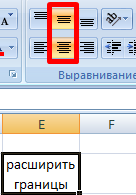
Для увеличения высоты строки можно нажать на панели инструментов кнопку «Перенос текста», или потянуть мышкой за границу на панели цифр-индексов.
С помощью кнопки «Распределение по вертикали» можно отобразить не помещающийся в ячейку текст в несколько строк.
Отмена внесенных изменений производится стандартным способом, с помощью кнопки «Отмена» или комбинации CTRL+Z. Желательно такие откаты делать сразу – потом это может и не сработать.

Если требуется отметить форматирование строк, можно воспользоваться вкладкой «Формат», в которой выбрать пункт «Автоподбор высоты строки».
Для отмены изменений размеров столбцов в той же вкладке «Формат» следует выбрать пункт «Ширина по умолчанию» — запоминаем стоящую здесь цифру, затем выделяем ту ячейку, границы которой были изменены и их нужно «вернуть». Теперь заходим в пункт «Ширина столбца» и вводим записанный на предыдущем шаге показатель по умолчанию.

Как вставить столбец/строку
Как обычно, вставку строки или столбца можно производить двумя способами, через вызов контекстного меню мышкой или с помощью горячих клавиш. В первом случае кликаем ПКМ на ячейке, которую необходимо сдвинуть, и в появившемся меню выбираем пункт «Добавить ячейки». Откроется стандартное окно, в котором можно задать, что именно вы хотите добавить, и будет указано, где произойдёт расширение (столбцы добавляются слева от текущей ячейки, строки – сверху).

Это же окно можно вызвать комбинацией CTRL+SHIFT+«=».
Столь подробное описание, как пользоваться программой Excel, несомненно, пригодится чайникам, то есть новичкам, ведь все эти манипуляции востребованы очень часто.

Пошаговое создание таблицы, вставка формул
Обычно в первой верхней строке с индексом 1 присутствуют наименования полей, или столбцов, а в строках вносятся отдельные записи. Поэтому первый шаг создания таблицы заключается в проставлении наименований столбцов (например, «Наименование товара», «Номер накладной», «Покупатель», «Количество», «Цена», «Сумма»).
После этого тоже вручную вносим данные по таблице. Возможно, в первом или третьем столбце нам придётся раздвигать границы – как это сделать/, мы уже знаем.

Теперь поговорим о вычисляемых значениях. В нашем случае это столбец «Сумма», который равен умножению количества на цену. В нашем случае столбец «Сумма» имеет букву F, столбцы «Количество» и «Цена» – D и E соответственно.
Итак, ставим курсор в ячейку F2 и набираем символ «=». Это означает, что в отношении всех ячеек в столбце F будут произведены вычисления согласно некоей формуле.

Чтобы ввести саму формулу, выделяем ячейку D2, жмём символ умножения, выделяем ячейку E2, жмём Enter. В результате в ячейке D2 появится число, равное произведению цены на количество. Чтобы формула работала для всех строк таблицы, цепляем мышкой в ячейке D2 левый нижний угол (при наведении на него появится маленький крестик) и тащим его вниз до конца. В итоге формула будет работать для всех ячеек, но со своим набором данных, взятым в той же строке.

Если нам нужно распечатать таблицу, то для придания читабельного вида строки и столбцы нужно ограничить сеткой. Для этого выделяем участок таблицы с данными, включая строку с наименованиями столбцов, выбираем вкладку «Границы» (она расположена в меню «Шрифт») и жмём на символе окошка с надписью «Все границы».
Вкладка «Шрифт» позволяет форматировать шрифты по тому же принципу, ВТО и в Word. Так, шапку лучше оформить жирным начертанием, текстовые столбцы лучше выравнивать по левому краю, а числа – центрировать. Итак, вы получили первые навыки, как работать в Excel. Перейдём теперь к рассмотрению других возможностей табличного процессора.

Как работать с таблицей Excel – руководство для чайников
Мы рассмотрели простейший пример табличных вычислений, в котором функция умножения вводилась вручную не совсем удобным способом.
Создание таблиц можно упростить, если воспользоваться инструментом под названием «Конструктор».
Он позволяет присвоить таблице имя, задать её размер, можно использовать готовые шаблоны, менять стили, есть возможность создания достаточно сложных отчётов.

Многие новички не могут понять, как скорректировать введённое в ячейку значение. При клике на ячейку, подлежащую изменению, и попытке ввода символов старое значение пропадает, и приходится всё вводить сначала. На самом деле значение ячейки при клике по ней появляется в статусной строке, расположенной под меню, и именно там и нужно редактировать её содержимое.
При вводе в ячейки одинаковых значений Excel проявляет интеллект, как поисковые системы – достаточно набрать несколько символов из предыдущей строки, чтобы её содержимое появилось в текущей – останется только нажать Enter или опуститься на строку ниже.

Синтаксис функций в Excel
Чтобы подсчитать итоги по столбцу (в нашем случае – общую сумму проданных товаров), необходимо поставить курсор в ячейку, в которой доложен находиться итог, и нажать кнопку «Автосумма» – как видим, ничего сложного, быстро и эффективно. Того же результата можно добиться, нажав комбинацию ALT+»=».
Ввод формул легче производить в статусной строке. Как только мы нажимаем в ячейке знак «=», он появляется и в ней, а слева от него имеется стрелка. Нажав на неё, мы получим список доступных функций, которые разбиты по категориям (математические, логические, финансовые, работа с текстом и т.д.). Каждая из функций имеет свой набор аргументов, которые нужно будет ввести. Функции могут быть вложенными, при выборе любой функции появится окошко с её кратким описанием, а после нажатия Ок – окно с необходимыми аргументами.

После завершения работы при выходе из программы она спросит, нужно ли сохранять внесённые вами изменения и предложит ввести имя файла.
Надеемся, приведённых здесь сведений достаточно для составления несложных таблиц. По мере освоения пакета Microsoft Excel вы будете узнавать новые его возможности, но мы утверждаем, что профессиональное изучение табличного процессора вам вряд ли потребуется. В сети и на книжных полках можно встретить книги и руководства из серии «Для чайников» по Excel на тысячи страниц. Сможете ли вы их осилить в полном объёме? Сомнительно. Тем более, что большинство возможностей пакета вам не потребуется. В любом случае мы будем рады ответить на ваши вопросы, касающиеся освоения самого известного табличного редактора.
Microsoft Excel – самая популярная программа для работы с электронными таблицами. Ее преимущество заключается в наличии всех базовых и продвинутых функций, которые подойдут как новичкам, так и опытным пользователям, нуждающимся в профессиональном ПО.
В рамках этой статьи я хочу рассказать о том, как начать работу в Эксель и понять принцип взаимодействия с данным софтом.
Создание таблицы в Microsoft Excel
Конечно, в первую очередь необходимо затронуть тему создания таблиц в Microsoft Excel, поскольку эти объекты являются основными и вокруг них строится остальная работа с функциями. Запустите программу и создайте пустой лист, если еще не сделали этого ранее. На экране вы видите начерченный проект со столбцами и строками. Столбцы имеют буквенное обозначение, а строки – цифренное. Ячейки образовываются из их сочетания, то есть A1 – это ячейка, располагающаяся под первым номером в столбце группы А. С пониманием этого не должно возникнуть никаких проблем.
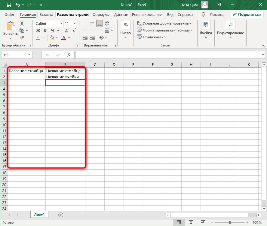
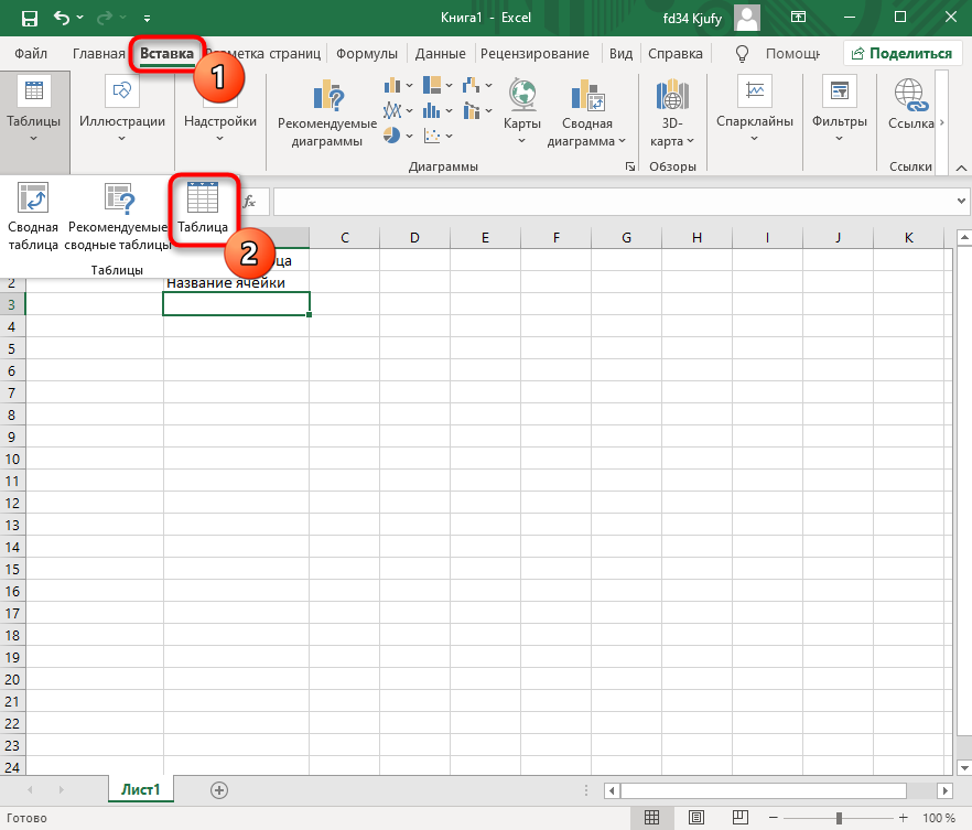
Обратите внимание на приведенный выше скриншот. Вы можете задавать любые названия для столбцов, заполняя данные в ячейках. Именно так формируется таблица. Если не ставить для нее границ, то она будет бесконечной. В случае необходимости создания выделенной таблицы, которую в будущем можно будет редактировать, копировать и связывать с другими листами, перейдите на вкладку «Вставка» и выберите вариант вставки таблицы.
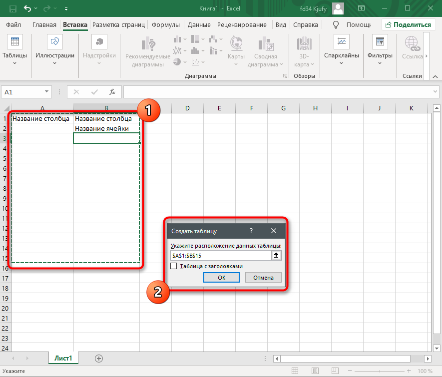
Задайте для нее необходимую область, зажав левую кнопку мыши и потянув курсор на необходимое расстояние, следя за тем, какие ячейки попадают в пунктирную линию. Если вы уже разобрались с названиями ячеек, можете заполнить данные самостоятельно в поле расположения. Однако там нужно вписывать дополнительные символы, с чем новички часто незнакомы, поэтому проще пойти предложенным способом. Нажмите «ОК» для завершения создания таблицы.
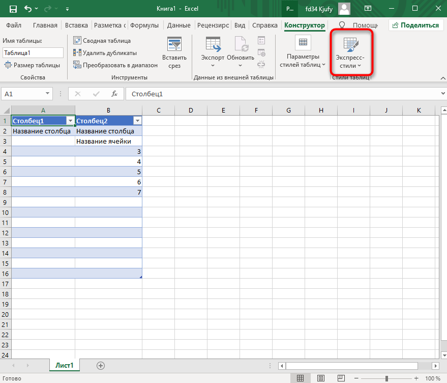
На листе вы сразу же увидите сформированную таблицу с группировками по столбцам, которые можно сворачивать, если их отображение в текущий момент не требуется. Видно, что таблица имеет свое оформление и точно заданные границы. В будущем вам может потребоваться увеличение или сокращение таблицы, поэтому вы можете редактировать ее параметры на вкладке «Конструктор».
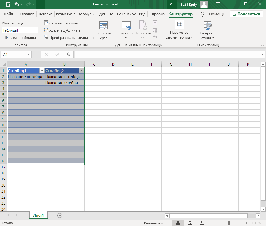
Обратите внимание на функцию «Экспресс-стили», которая находится на той же упомянутой вкладке. Она предназначена для изменения внешнего вида таблицы, цветовой гаммы. Раскройте список доступных тем и выберите одну из них либо приступите к созданию своей, разобраться с чем будет не так сложно.
Комьюнити теперь в Телеграм
Подпишитесь и будьте в курсе последних IT-новостей
Подписаться
Основные элементы редактирования
Работать в Excel самостоятельно – значит, использовать встроенные элементы редактирования, которые обязательно пригодятся при составлении таблиц. Подробно останавливаться на них мы не будем, поскольку большинство из предложенных инструментов знакомы любому пользователю, кто хотя бы раз сталкивался с подобными элементами в том же текстовом редакторе от Microsoft.
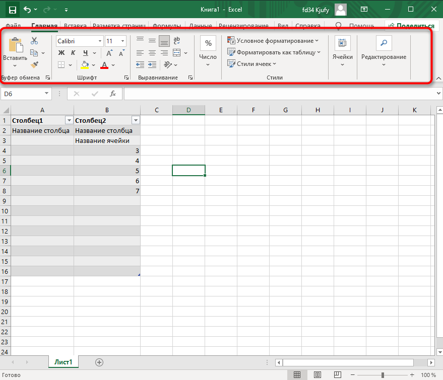
На вкладке «Главная» вы увидите все упомянутые инструменты. С их помощью вы можете управлять буфером обмена, изменять шрифт и его формат, использовать выравнивание текста, убирать лишние знаки после запятой в цифрах, применять стили ячеек и сортировать данные через раздел «Редактирование».
Использование функций Excel
По сути, создать ту же таблицу можно практически в любом текстовом или графическом редакторе, но такие решения пользователям не подходят из-за отсутствия средств автоматизации. Поэтому большинство пользователей, которые задаются вопросом «Как научиться работать в Excel», желают максимально упростить этот процесс и по максимуму задействовать все встроенные инструменты. Главные средства автоматизации – функции, о которых и пойдет речь далее.
-
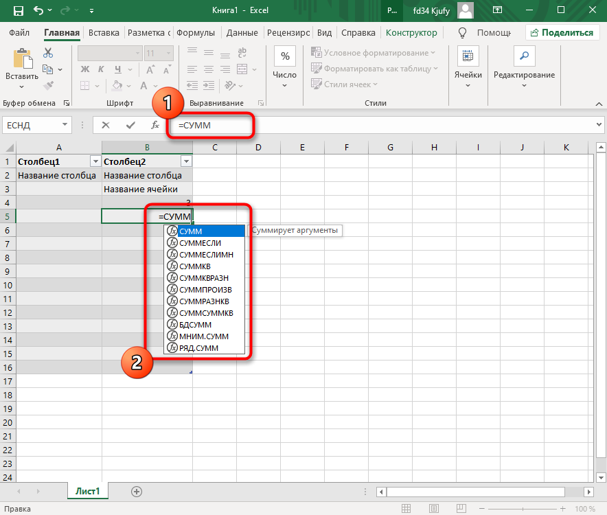
Если вы желаете объявить любую функцию в ячейке (результат обязательно выводится в поле), начните написание со знака «=», после чего впишите первый символ, обозначающий название формулы. На экране появится список подходящих вариантов, а нажатие клавиши TAB выбирает одну из них и автоматически дописывает оставшиеся символы.
-
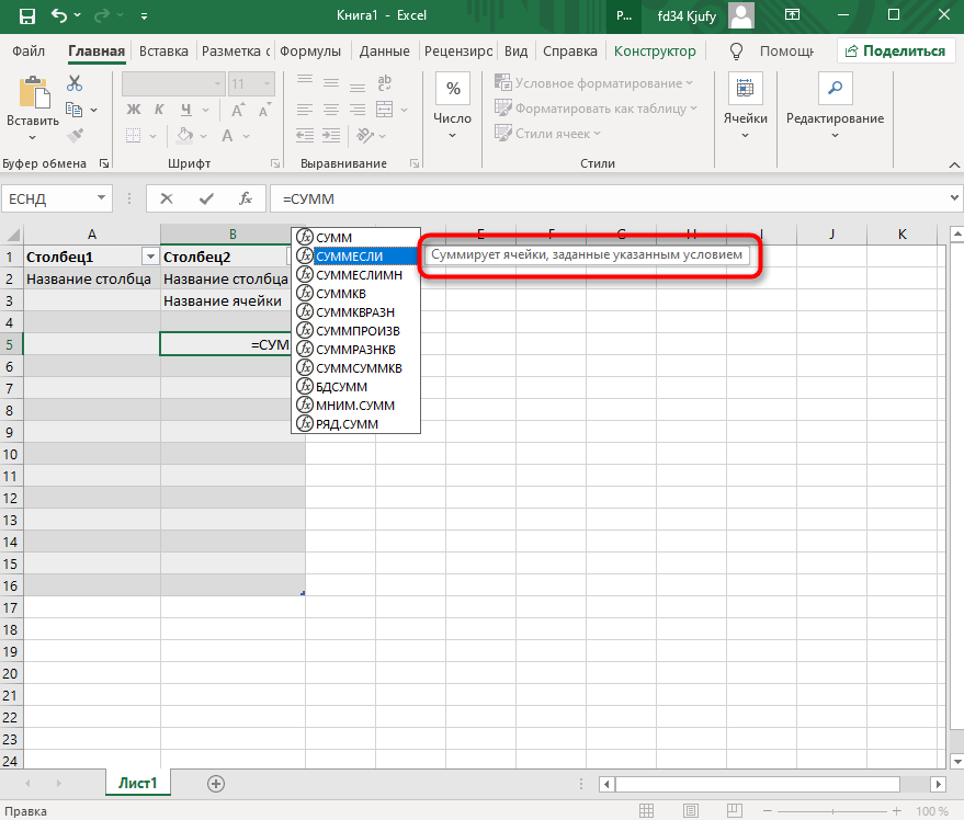
Обратите внимание на то, что справа от имени выбранной функции показывается ее краткое описание от разработчиков, позволяющее понять предназначение и действие, которое она выполняет.
-
Если кликнуть по значку с функцией справа от поля ввода, на экране появится специальное окно «Вставка функции», в котором вы можете ознакомиться со всеми ними еще более детально, получив полный список и справку. Если выбрать одну из функций, появится следующее окно редактирования, где указываются аргументы и опции. Это позволит не запутаться в правильном написании значений.
-
Взгляните на следующее изображение. Это пример самой простой функции, результатом которой является сумма указанного диапазона ячеек или двух из них. В данном случае знак «:» означает, что все значения ячеек указанного диапазона попадают под выражение и будут суммироваться. Все формулы разобрать в одной статье нереально, поэтому читайте официальную справку по каждой или найдите открытую информацию в сети.
-
На вкладке с формулами вы можете найти любую из них по группам, редактировать параметры вычислений или зависимости. В большинстве случаев это пригождается только опытным пользователям, поэтому просто упомяну наличие такой вкладки с полезными инструментами.
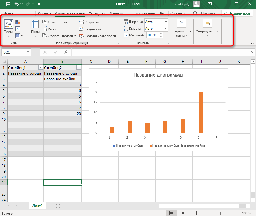
Вставка диаграмм
Часто работа в Эксель подразумевает использование диаграмм, зависимых от составленной таблицы. Обычно это требуется ученикам, которые готовят на занятия конкретные проекты с вычислениями, однако применяются графики и в профессиональных сферах. На данном сайте есть другая моя инструкция, посвященная именно составлению диаграммы по таблице. Она поможет разобраться во всех тонкостях этого дела и самостоятельно составить график необходимого типа.
Подробнее: Как построить диаграмму по таблице в Excel: пошаговая инструкция
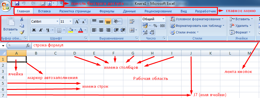
Элементы разметки страницы
Вкладка под названием «Разметка страницы» пригодится вам только в том случае, если создаваемый лист в будущем должен отправиться в печать. Здесь вы найдете параметры страницы, сможете изменить ее размер, ориентацию, указать область печати и выполнить другое редактирование. Большинство доступных инструментов подписаны, и с их использованием не возникнет никаких проблем. Учитывайте, что при внесении изменений вы можете нажать комбинацию клавиш Ctrl + Z, если вдруг что-то сделали не так.
Сохранение и переключение между таблицами
Программа Эксель подразумевает огромное количество мелочей, на разбор которых уйдет ни один час времени, однако начинающим пользователям, желающим разобраться в базовых вещах, представленной выше информации будет достаточно. В завершение отмечу, что на главном экране вы можете сохранять текущий документ, переключаться между таблицами, отправлять их в печать или использовать встроенные шаблоны, когда необходимо начать работу с заготовками.

Надеюсь, что эта статья помогла разобраться вам с тем, как работать в Excel хотя бы на начальном уровне. Не беспокойтесь, если что-то не получается с первого раза. Воспользуйтесь поисковиком, введя там запрос по теме, ведь теперь, когда имеются хотя бы общие представления об электронных таблицах, разобраться в более сложных вопросах будет куда проще.
Microsoft Excel – чрезвычайно полезная программка в разных областях. Готовая таблица с возможностью автозаполнения, быстрых расчетов и вычислений, построения графиков, диаграмм, создания отчетов или анализов и т.д.
Инструменты табличного процессора могут значительно облегчить труд специалистов из многих отраслей. Представленная ниже информация – азы работы в Эксель для чайников. Освоив данную статью, Вы приобретете базовые навыки, с которых начинается любая работа в Excel.
Инструкция по работе в Excel
Книга Excel состоит из листов. Лист – рабочая область в окне. Его элементы:
Чтобы добавить значение в ячейку, щелкаем по ней левой кнопкой мыши. Вводим с клавиатуры текст или цифры. Жмем Enter.
Значения могут быть числовыми, текстовыми, денежными, процентными и т.д. Чтобы установить/сменить формат, щелкаем по ячейке правой кнопкой мыши, выбираем «Формат ячеек». Или жмем комбинацию горячих клавиш CTRL+1.
Для числовых форматов можно назначить количество десятичных знаков.
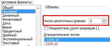
Примечание. Чтобы быстро установить числовой формат для ячейки — нажмите комбинацию горячих клавиш CTRL+SHIFT+1.
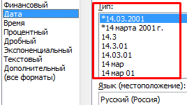
Для форматов «Дата» и «Время» Excel предлагает несколько вариантов изображения значений.
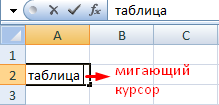
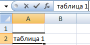
Отредактируем значение ячеек:
- Щелкнем по ячейке со словом левой кнопкой мыши и введем число, например. Нажимаем ВВОД. Слово удаляется, а число остается.
- Чтобы прежнее значение осталось, просто изменилось, нужно щелкнуть по ячейке два раза. Замигает курсор. Меняем значение: удаляем часть текста, добавляем.
- Отредактировать значения можно и через строку формул. Выделяем ячейку, ставим курсор в строку формул, редактируем текст (число) – нажимаем Enter.
Для удаления значения ячейки используется кнопка Delete.
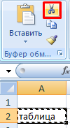
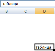
Чтобы переместить ячейку со значением, выделяем ее, нажимаем кнопку с ножницами («вырезать»). Или жмем комбинацию CTRL+X. Вокруг ячейки появляется пунктирная линия. Выделенный фрагмент остается в буфере обмена.
Ставим курсор в другом месте рабочего поля и нажимаем «Вставить» или комбинацию CTRL+V.
Таким же способом можно перемещать несколько ячеек сразу. На этот же лист, на другой лист, в другую книгу.
Чтобы переместить несколько ячеек, их нужно выделить:
- Ставим курсор в крайнюю верхнюю ячейку слева.
- Нажимаем Shift, удерживаем и с помощью стрелок на клавиатуре добиваемся выделения всего диапазона.
Чтобы выделить столбец, нажимаем на его имя (латинскую букву). Для выделения строки – на цифру.
Для изменения размеров строк или столбцов передвигаем границы (курсор в этом случае принимает вид крестика, поперечная перекладина которого имеет на концах стрелочки).
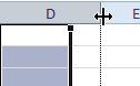
Чтобы значение поместилось в ячейке, столбец можно расширить автоматически: щелкнуть по правой границе 2 раза.
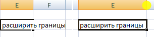
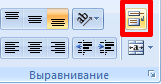
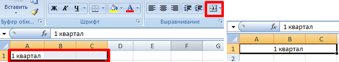
Чтобы сохранить ширину столбца, но увеличить высоту строки, нажимаем на ленте кнопок «Перенос текста».
Чтобы стало красивее, границу столбца Е немного подвинем, текст выровняем по центру относительно вертикали и горизонтали.
Объединим несколько ячеек: выделим их и нажмем кнопку «Объединить и поместить в центре».
В Excel доступна функция автозаполнения. Вводим в ячейку А2 слово «январь». Программа распознает формат даты – остальные месяцы заполнит автоматически.
Цепляем правый нижний угол ячейки со значением «январь» и тянем по строке.
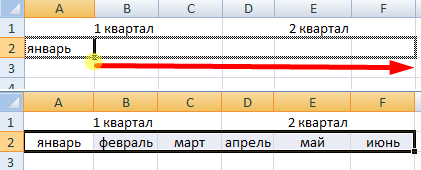
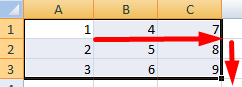
Апробируем функцию автозаполнения на числовых значениях. Ставим в ячейку А3 «1», в А4 – «2». Выделяем две ячейки, «цепляем» мышью маркер автозаполнения и тянем вниз.
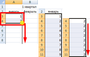
Если мы выделим только одну ячейку с числом и протянем ее вниз, то это число «размножиться».
Чтобы скопировать столбец на соседний, выделяем этот столбец, «цепляем» маркер автозаполнения и тянем в сторону.
Таким же способом можно копировать строки.
Удалим столбец: выделим его – правой кнопкой мыши – «Удалить». Или нажав комбинацию горячих клавиш: CTRL+»-«(минус).
Чтобы вставить столбец, выделяем соседний справа (столбец всегда вставляется слева), нажимаем правую кнопку мыши – «Вставить» — «Столбец». Комбинация: CTRL+SHIFT+»=»
Чтобы вставить строку, выделяем соседнюю снизу. Комбинация клавиш: SHIFT+ПРОБЕЛ чтобы выделить строку и нажимаем правую кнопку мыши – «Вставить» — «Строку» (CTRL+SHIFT+»=»)(строка всегда вставляется сверху).
Как работать в Excel: формулы и функции для чайников
Чтобы программа воспринимала вводимую в ячейку информацию как формулу, ставим знак «=». Например, = (2+3)*5. После нажатия «ВВОД» Excel считает результат.
Последовательность вычисления такая же, как в математике.
Формула может содержать не только числовые значения, но и ссылки на ячейки со значениями. К примеру, =(A1+B1)*5, где А1 и В1 – ссылки на ячейки.
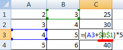
Чтобы скопировать формулу на другие ячейки, необходимо «зацепить» маркер автозаполнения в ячейке с формулой и протянуть вниз (в сторону – если копируем в ячейки строки).
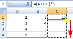
При копировании формулы с относительными ссылками на ячейки Excel меняет константы в зависимости от адреса текущей ячейки (столбца).
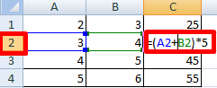
Чтобы сделать ссылку абсолютной (постоянной) и запретить изменения относительно нового адреса, ставится знак доллара ($).
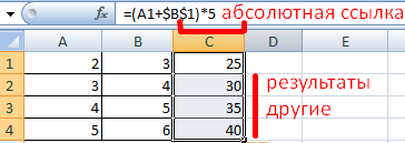
В каждой ячейке столбца С второе слагаемое в скобках – 3 (ссылка на ячейку В1 постоянна, неизменна).
Значительно расширяют функционал программы встроенные функции. Чтобы вставить функцию, нужно нажать кнопку fx (или комбинацию клавиш SHIFT+F3). Откроется окно вида:
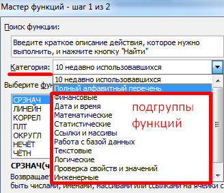
Чтобы не листать большой список функций, нужно сначала выбрать категорию.
Когда функция выбрана, нажимаем ОК. Откроется окно «Аргументы функции».
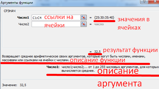
Функции распознают и числовые значения, и ссылки на ячейки. Чтобы поставить в поле аргумента ссылку, нужно щелкнуть по ячейке.
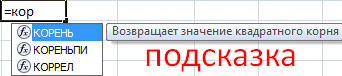
Excel распознает и другой способ введения функции. Ставим в ячейку знак «=» и начинаем вводить название функции. Уже после первых символов появится список возможных вариантов. Если навести курсор на какой-либо из них, раскроется подсказка.
Дважды щелкаем по нужной функции – становится доступным порядок заполнения аргументов. Чтобы завершить введение аргументов, нужно закрыть скобку и нажать Enter.
Аргумент функции КОРЕНЬ – ссылка на ячейку A1:
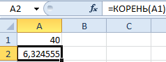
ВВОД – программа нашла квадратный корень из числа 40.
In an article written in 2018, Robert Half, a company specializing in human resources and the financial industry, wrote that 63% of financial firms continue to use Excel in a primary capacity. Granted, that is not 100% and is actually considered to be a decline in usage! But considering the software is a spreadsheet software and not designed solely as financial industry software, 63% is still a significant portion of the industry and helps to illustrate how important Excel is.
Learning how to use Excel doesn’t have to be difficult. Taking it one step at a time will help you move from a novice to an expert (or at least closer to that point) – at your pace.

As a preview of what we are going to cover in this article, think worksheets, basic usable functions and formulas, and navigating a worksheet or workbook. Granted, we will not be covering every possible Excel function but we will cover enough that it gives you an idea of how to approach the others.
Basic Definitions
It really is helpful if we cover a few definitions. More than likely, you have heard these terms (or already know what they are). But we will cover them to be sure and be all set for the rest of the process in learning how to use Excel.
Workbooks vs. Worksheets
Excel documents are called Workbooks and when you first create an Excel document (the workbook), many (not all) Excel versions will automatically include three tabs, each with its own blank worksheet. If your version of Excel doesn’t do that, don’t worry, we will learn how to create them.
The Worksheets are the actual parts where you enter the data. If it is easier to think of it visually, think of the worksheets as those tabs. You can add tabs or delete tabs by right-clicking and choosing the delete option. Those worksheets are the actual spreadsheets with which we work and they are housed in the workbook file.
The Ribbon
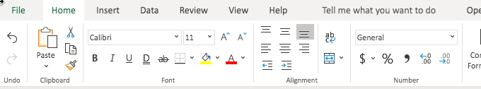
The Ribbon spreads across the Excel application like a row of shortcuts, but shortcuts that are represented visually (with text descriptions). This is helpful when you want to do something in short order and especially when you need help determining what you want to do.
There is a different grouping of ribbon buttons depending on which section/group you choose from the top menu options (i.e. Home, Insert, Data, Review, etc.) and the visual options presented will relate to those groupings.
Excel Shortcuts
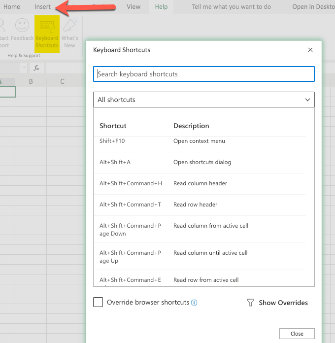
Shortcuts are helpful in navigating the Excel software quickly, so it is helpful (but not absolutely essential) to learn them. Some of them are learned by seeing the shortcuts listed in the menus of the older versions of the Excel application and then trying them out for yourself.
Another way to learn Excel shortcuts is to view a list of them on the website of the Excel developers. Even if your version of Excel doesn’t display the shortcuts, most of them still work.
Formulas vs. Functions
Functions are built-in capabilities of Excel and are used in formulas. For example, if you wanted to insert a formula that calculated the sum of numbers in different cells of a spreadsheet, you could use the function SUM() to do just that.
More on this function (and other functions) a bit further on in this article.
Formula Bar

The formula bar is an area that appears below the Ribbon. It is used for formulas and data. You enter the data in the cell and it will also appear in the formula bar if you have your mouse on that cell.
When we reference the formula bar, we are simply indicating that we should type the formula in that spot while having the appropriate cell selected (which, again, will automatically happen if you select the cell and start typing).
Creating & Formatting a Worksheet Example
There are many things you can do with your Excel Worksheet. We will give you some example steps as we go along in this article so you can try them out for yourself.
The First Workbook
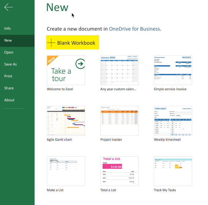
It is helpful to start with a blank Workbook. So, go ahead and select New. This may vary, depending on your version of Excel, but is generally in the File area.

Note: The above image says Open at the top to illustrate that you can get to the New (left-hand side, pointed to with the green arrow) from anywhere. This is a screenshot of the newer Excel.
When you click on New you are more than likely going to get some example templates. The templates themselves may vary between versions of Excel, but you should get some sort of selection.
One way of learning how to use Excel is to play with those templates and see what makes them “tick”. For our article, we are starting with a blank document and playing around with data and formulas, etc.
So go ahead and select the blank document option. The interface will vary, from version to version, but should be similar enough to get the idea. A little later we will also download another sample Excel sheet.
Inserting the Data
There are many different ways to get data into your spreadsheet (a.k.a. worksheet). One way is to simply type what you want where you want it. Choose the particular cell and just start typing.
Another way is to copy data and then paste it into your Spreadsheet. Granted, if you are copying data that is not in a table format it can get a little interesting as to where it lands in your document. But fortunately we can always edit the document and recopy and paste elsewhere, as needed.
You can try the copy/paste method now by selecting a portion of this article, copying it, and then pasting into your blank spreadsheet.
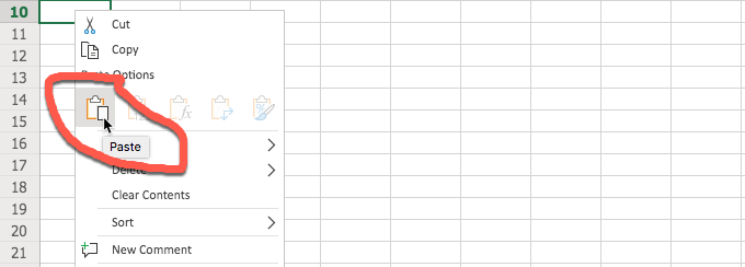
After selecting the portion of the article and copying it, go to your spreadsheet and click on the desired cell where you want to start the paste and do so. The method shown above is using the right-click menu and then selecting “Paste” in the form of the icon.
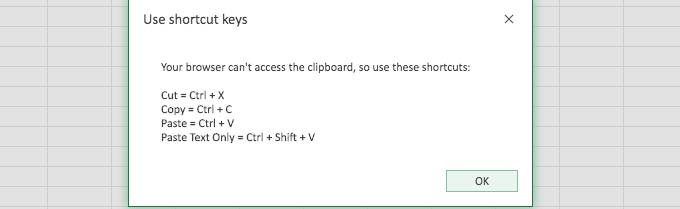
It is possible that you may get an error when using the Excel built-in paste method, even with the other Excel built-in methods as well. Fortunately, the error warning (above) helps to point you in the right direction to get the data you copied into the sheet.
When pasting the data, Excel does a pretty good job of interpreting it. In our example, I copied the first two paragraphs of this section and Excel presented it in two rows. Since there was an actual space between the paragraphs, Excel reproduced that as well (with a blank row). If you are copying a table, Excel does an even better job of reproducing it in the sheet.

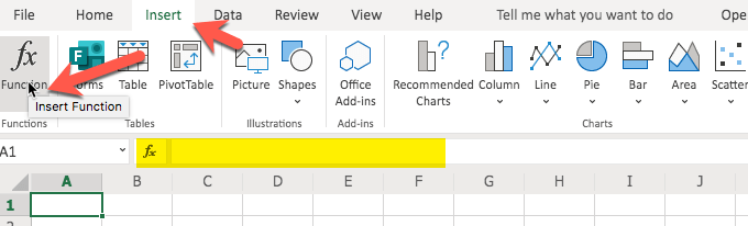
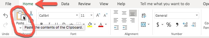
Also, you can use the button in the Ribbon to paste. For visual people, this is really helpful. It is shown in the image below.
Some versions of Excel (especially the older versions) allow you to import data (which works best with similar files or CSV – comma-separated values – files). Some newer versions of Excel do not have that option but you can still open the other file (the one that you want to import), use a select all and then copy and paste it into your Excel spreadsheet.
When import is available, it is generally found under the File menu. In the new version(s) of Excel, you may be rerouted to more of a graphical user interface when you click on File. Simply click the arrow in the top left to return back to your worksheet.
Hyperlinking
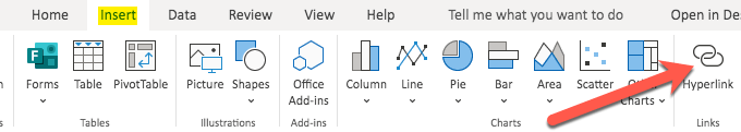
Hyperlinking is fairly easy, especially when using the Ribbon. You will find the hyperlink button under the Insert menu in the newer Excel versions. It may also be accessed via a shortcut like command-K.
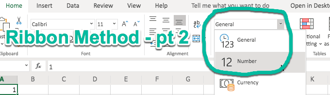
Formatting Data (Example: Numbers and Dates)
Sometimes it is helpful to format the data. This is especially true with numbers. Why? Sometimes numbers automatically fall into a general format (sort of default) which is more like a text format. But often, we want our numbers to behave as numbers.
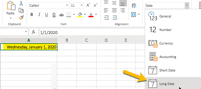
The other example would be dates, which we may want to format to ensure that all of our dates appear consistent, like 20200101 or 01/01/20 or whatever format we choose for our date format.
You can access the option to format your data in a couple of different ways, shown in the below images.
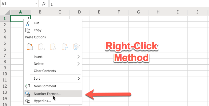
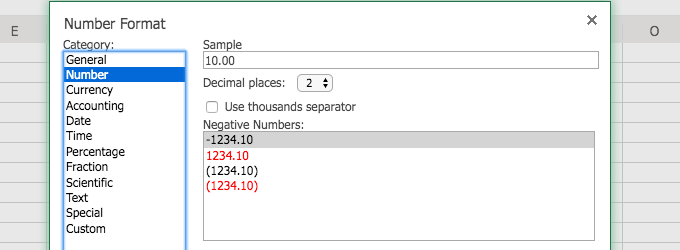
Once you have accessed, say, the Number format, you will have several options. These options appear when you use the right-click method. When you use the Ribbon, your options are right there in the Ribbon. It all depends on which is easier for you.
If you have been using Excel for a while, the right-click method, with the resulting number format dialog box (shown below) may be easier to understand. If you are newer or more visual, the Ribbon method may make more sense (and much quicker to use). Both provide you with number formatting options.
If you type anything that resembles a date, the newer versions of Excel are nice enough to reflect that in the Ribbon as shown in the below image.
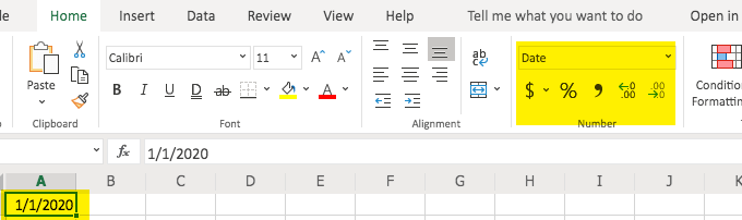
From the Ribbon you can select formats for your date. For example, you can choose a short date or a long date. Go ahead and try it and view your results.
Presentation Formatting (Example: Aligning Text)
It is also helpful to understand how to align your data, whether you want it all to line up to the left or to the right (or justified, etc). This too can be accessed via the Ribbon.
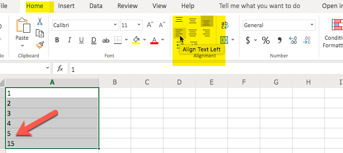
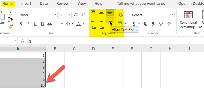
As you can see from the images above, the alignment of the text (i.e. right, left, etc.) is on the second row of the Ribbon option. You can also choose other alignment options (i.e. top, bottom) in the Ribbon.
Also, if you notice, aligning things like numbers may not look right when aligned left (where text looks better) but does look better when aligned right. The alignment is very similar to what you would see in a word processing application.
Columns & Rows
It is helpful to know how to work with, as well as adjust the width and dimensions of, columns and rows. Fortunately, once you get the hang of it, it is fairly easy to do.
There are two parts to adding or deleting rows or columns. The first part is the selection process and the other is the right-click and choosing the insert or delete option.
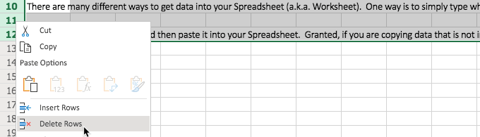
Remember the data we copied from this article and pasted into our blank Excel sheet in the above example? We probably don’t need it anymore so it is a perfect example for the process of deleting rows.
Remember our first step? We need to select the rows. Go ahead and click on the row number (to the left of the top left cell) and drag downward with your mouse to the bottom row that you want to delete. In this case, we are selecting three rows.
Then, the second part of our procedure is to click on Delete Rows and watch Excel delete those rows.

The process for inserting a row is similar but you do not have to select more than one row. Excel will determine where you click is where you want to insert the row.
To start the process, click on the row number that you want to be below the new row. This tells Excel to select the entire row for you. From the spot where you are, Excel will insert the row above that. You do so by right-clicking and choosing Insert Rows.
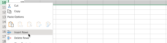
As you can see above, we typed 10 in row 10. Then, after selecting 10 (row 10), right-clicking, and choosing Insert Rows, the number 10 went down one row. It resulted in the 10 now being in row 11.
This demonstrates how the inserted row was placed above the selected row. Go ahead and try it for yourself, so you can see how the insertion process works.
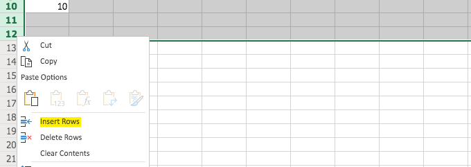
If you need more than one row, you can do so by selecting more than one row and this tells Excel how many you want and that quantity will be inserted above the row number selected.
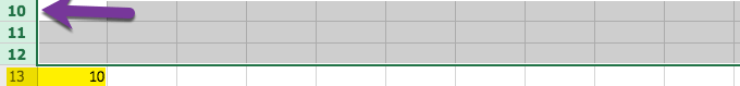
The following pictures show this in a visual format, including how the 10 went down three rows, the number of rows inserted.
Inserting and deleting columns is basically the same except that you are selecting from the top (columns) instead of the left (rows).
Filters & Duplicates
When we have a lot of data to work with it helps if we have a couple of tricks up our sleeves in order to more easily work with that data.
For example, let’s say you have a bunch of financial data but you only need to look at specific data. One way to do that is to use an Excel “Filter.”
First, let’s find an Excel Worksheet that presents a lot of data so we have something to test this on (without having to type all of the data ourselves). You can download just such a sample from Microsoft. Keep in mind that that is the direct link to the download so the Excel example file should start downloading right away when you click on that link.
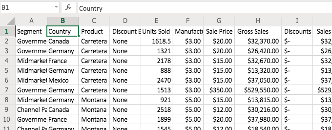
Now that we have the document, let’s look at the volume of data. Quite a bit, isn’t it? Note: the image above will look a bit different from what you have in your sample file and that is normal.
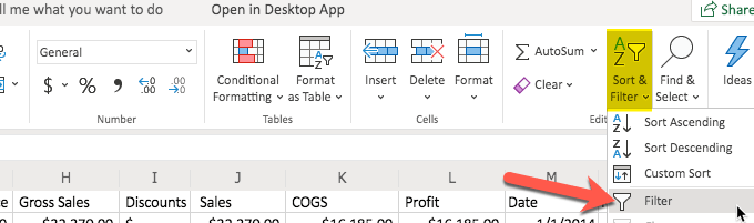
Let’s say you only wanted to see data from Germany. Use the “Filter” option in the Ribbon (under “Home”). It is combined with the “Sort” option towards the right (in the newer Excel versions).
Now, tell Excel what options you want. In this case, we are looking for data on Germany as the selected country.
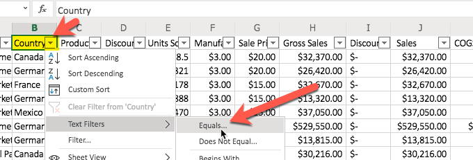
You will notice that when you select the filter option, little pull-down arrows appear in the columns. When an arrow is selected, you have several options, including the “Text Filters” option that we will be using. You have an option to sort ascending or descending.
It makes sense why Excel combines these in the Ribbon since all of these options appear in the pull-down list. We will be selecting the “Equals…” under the “Text Filters.”
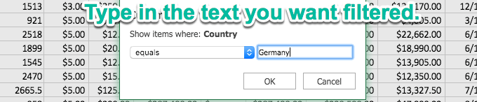
After we select what we want to do (in this case Filter), let’s provide the information/criteria. We would like to see all the data from Germany so that is what we type in the box. Then, click “OK.”
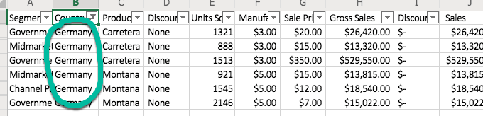
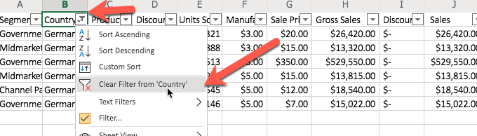
You will notice that now we only see data from Germany. The data has been filtered. The other data is still there. It is just hidden from view. There will come a time when you want to discontinue the filter and see all of the data. Simply return to the pull-down and choose to clear the filter, as shown in the below image.
Sometimes you will have data sets that include duplicate data. It is much easier if you only have singular data. For example, why would you want the exact same financial data record twice (or more) in your Excel Worksheet?
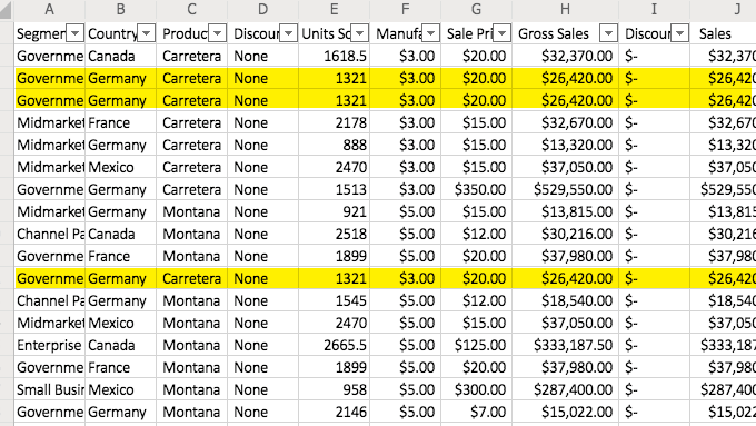
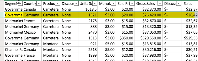
Below is an example of a data set that has some data that is repeated (shown highlighted in yellow).
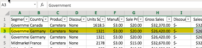
To remove duplicates (or more, as in this case), start by clicking on one of the rows that represents the duplicate data (that contains the data that is repeated). This is shown in the below image.
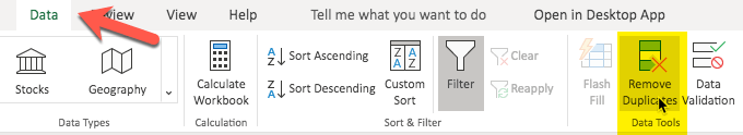
Now, visit the “Data” tab or section and from there, you can see a button on the Ribbon that says “Remove Duplicates.” Click that.
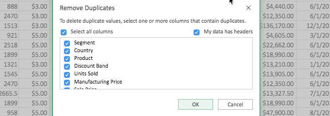
The first portion of this process presents you with a dialog box similar to what you see in the below image. Don’t let this confuse you. It is simply asking you which column to look at when identifying the duplicate data.
For example, if you had several rows with the same first and last name but basically gibberish in the other columns (like a copy/paste from a website for example) and you only needed unique rows for the first and last name, you would select those columns so that the gibberish that may not be duplicate does not come into consideration in removing the excess data.
In this case, we left the selection as “all columns” because we had duplicated rows manually so we knew that all of the columns were exactly the same in our example. (You can do the same with the Excel example file and test it.)
After you click “OK” on the above dialog box, you will see the result and in this case, three rows were identified as matching and two of them were removed.
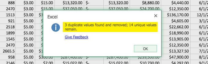
Now, the resulting data (shown below) matches the data we started with before we went through the addition and removal of duplicates.
You have just learned a couple tricks. These are especially helpful when dealing with larger data sets. Go ahead and try some other buttons that you see on the Ribbon and see what they do. You can also duplicate your Excel example file if you want to retain the original form. Rename the file you downloaded and re-download another copy. Or duplicate the file on your computer.
What I did was duplicate the tab with all of the financial data (after copying it into my other example file, the one we started with that was blank) and with the duplicate tab I had two versions to play with at will. You can try this by using the right-click on the tab and choosing “Duplicate.”
Conditional Formatting
This part of the article is included in the section on creating the Workbook because of its display benefits. If it seems a little complicated or you are looking for functions and formulas, skip this section and come back to it at your leisure.
Conditional Formatting is handy if you want to highlight certain data. In this example, we are going to use our Excel Example file (with all of the financial data) and look for the “Gross Sales” that are over $25,000.
In order to do this, we first have to highlight the group of cells that we want evaluated. Now, keep in mind, you do not want to highlight the entire column or row. You only want to highlight just the cells that you want evaluated. Otherwise, the other cells (like headings) will also be evaluated and you would be surprised what Excel does with those headings (as an example).
So, we have our desired cells highlighted and now we click on the “Home” section/group and then “Conditional Formatting.”
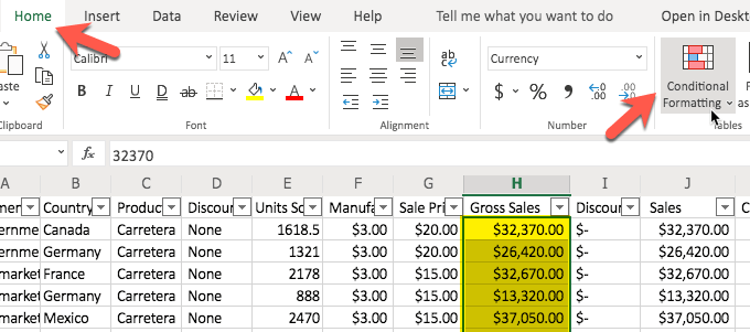
When we click on “Conditional Formatting” in the Ribbon, we have some options. In this case we want to highlight the cells that are greater than $25,000 so that is how we make our selection, as shown in the below image.
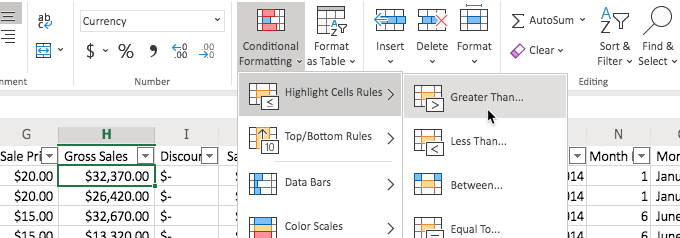
Now we will see a dialog box and we can type the value in the box. We type 25000. You don’t have to worry about commas or anything and in fact, it works better if you just type in the raw number.
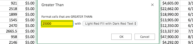
After we click “OK” we will see that the fields are automatically colored according to our choice (to the right) in our “Greater Than” above dialog box. In this case, “Light Red Fill with Dark Red Text). We could have chosen a different display option as well.
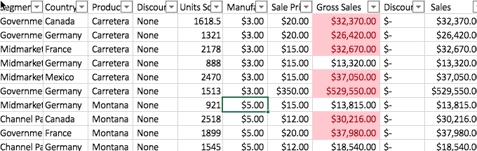
This conditional formatting is a great way to see, at a glance, data that is essential for one project or another. In this case, we could see the “Segments” (as they are referred to in the Excel Example file) that have been able to exceed $25,000 in Gross Sales.
Working With Formulas and Functions
Learning how to use functions in Excel is very helpful. They are the basic guts of the formulas. If you want to see a listing of the functions to get an idea of what is available, click on the “Insert” menu/group and then at the far left, choose “Function/Functions.”
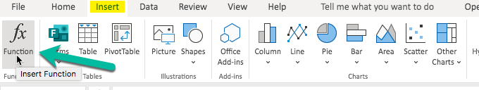
Even though the purpose of this button in the Excel Ribbon is to insert an actual function (which can also be accomplished by typing in the formula bar, starting with an equals sign and then starting to type the desired function), we can also use this to see what is available. You can scroll through the functions to get a sort of idea of what you can use in your formulas.
Granted, it is also very helpful to simply try them out and see what they do. You can select the group that you want to peruse by choosing a category, like “Commonly Used” for a shorter list of functions but a list that is often used (and for which some functions are covered in this article).
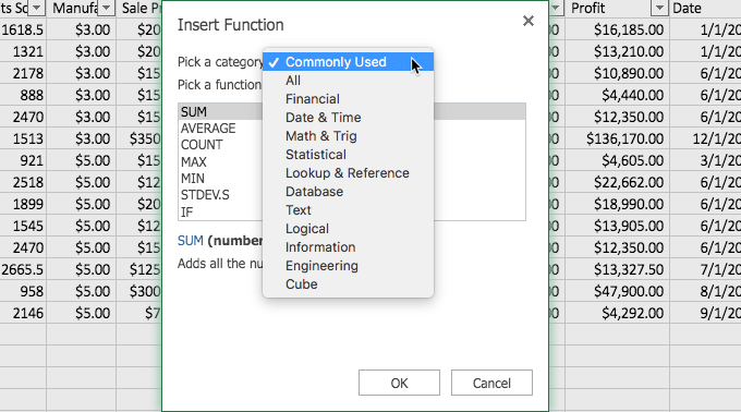
We will be using some of these functions in the examples of the formulas we discuss in this article.
The Equals = Sign
The equals sign ( = ) is very important in Excel. It plays an essential role. This is especially true in the cases of formulas. Basically, you don’t have a formula without preceding it with an equals sign. And without the formula, it is simply the data (or text) you have entered in that cell.
So just remember that before you are asking Excel to calculate or automate anything for you, that you type an equals sign ( = ) in the cell.

If you include a $ sign, that tells Excel not to move the formula. Normally, the auto adjustment of formulas (using what is called relative cell references), to changes in the worksheet, is a helpful thing but sometimes you may not want it and with that $ sign, you are able to tell Excel that. You simply insert the $ in front of the letter and number of the cell reference.
So a relative cell reference of D25 becomes $D$25. If this part is confusing, don’t worry about it. You can come back to it (or play with it with an Excel blank workbook).
The Awesome Ampersand >> &
The ampersand ( & ) is a fun little formula “tool,” allowing you to combine cells. For example, let’s say that you have a column for first names and another column for last names and you want to create a column for the full name. You can use the & to do just that.
Let’s try it in an Excel Worksheet. For this example, let’s use a blank sheet so we don’t interrupt any other project. Go ahead and type your first name in A1 and type your last name in B1. Now, to combine them, click your mouse on the C1 cell and type this formula: =A1 & “ “ & B1. Please only use the part in italics and not any of the rest of it (like not using the period).
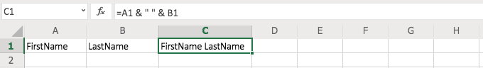
What do you see in C1? You should see your full name complete with a space between your first and last names, as would be normal in typing your full name. The & “ “ & portion of the formula is what produced that space. If you had not included “ “ you would have had your first name and last name without a space between them (go ahead and try it if you want to see the result).
Another similar formula uses CONCAT but we will learn about that a little later. For now, keep in mind what the ampersand ( & ) can do for you as this little tip comes in handy in many situations.
SUM() Function
The SUM() function is very handy and it does just what it describes. It adds up the numbers you tell Excel to include and gives you the sum of their values. You can do this in a couple of different ways.
We started by typing in some numbers so we had some data to work with in the use of the function. We simply used 1, 2, 3, 4, 5 and started in A1 and typed in each cell going downward toward A5.
Now, to use the SUM() function, start by clicking in the desired cell, in this case we used A6, and typing =SUM( in the formula bar. In this example, stop when you get to the first “(.” Now, click in A1 (the top-most cell) and drag your mouse to A5 (or the bottom-most cell you want to include) and then return to the formula bar and type the closing “).” Do not include the periods or quotation marks and just the parentheses.
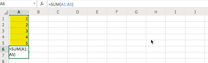
The other way to use this function is to manually type the information in the formula bar. This is especially helpful if you have quite a few numbers and scrolling to grab them is a bit difficult. Start this method the same way that you did for the example above, with “=SUM(.”
Then, type the top-most cell’s cell reference. In this case, that would be A1. Include a colon ( : ) and then type the bottom-most cell’s cell reference. In this case, that would be A5.
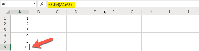
AVERAGE() Function
What if you wanted to figure out what the average of a group of numbers was? You can easily do that with the AVERAGE() function. You will notice, in the steps below, that it is basically the same as the SUM() function above but with a different function.
With that in mind, we start by selecting the cell we want to use for the result (in this case A6) and then start typing with an equals sign ( = ) and the word AVERAGE. You will notice that as you begin typing it you are offered suggestions and can click on AVERAGE instead of typing the full word, if you like.
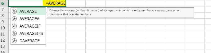
Ensure that you have an opening parenthesis in your formula before we add our cell range. Otherwise, you will receive an error.
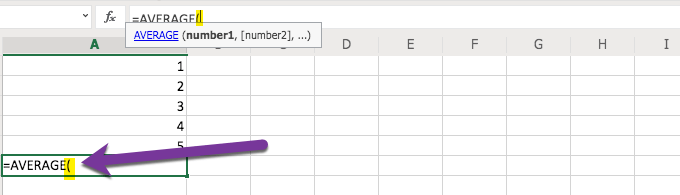
Now that we have “=AVERAGE(“ typed in our A6 cell (or whichever cell you are using for the result) we can select the cell range that we want to use. In this case we are using A1 through A5.
Keep in mind that you can also type it in manually rather than using the mouse to select the range. If you have a large data set typing in the range is probably easier than the scrolling that would be required to select it. But, of course, it is up to you.
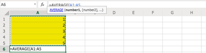
To complete the process simply type in the closing parenthesis “)” and you will receive the average of the five numbers. As you can see, this process is very similar to the SUM() process and other functions. Once you get the hang of one function, the others will be easier.
COUNTIF() Function
Let’s say we wanted to count how many times a certain number shows up in a data set. First, let’s prepare our file for this function so that we have something to count. Remove any formula that you may have in A6. Now, either copy A1 through A5 and paste starting in A6 or simply type the same numbers in the cells going downward starting with A6 and the value of 1 and then A7 with 2, etc.
Now, in A11 let’s start our function/formula. In this case, we are going to type “=COUNTIF(.” Then, we will select cells A1 through A10.
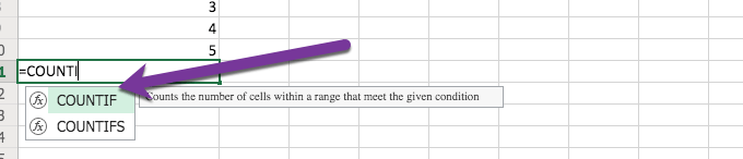
Be sure that you type or select “COUNTIF” and not one of the other COUNT-like functions or we will not get the same result.
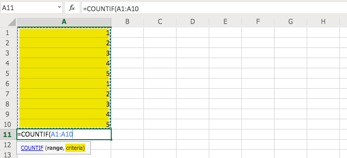
Before we do like we have with our other functions, and type the closing parenthesis “)” we need to answer the question of criteria and type that, after a comma “,” and before the parenthesis “).”
What is defined by the “criteria?” That is where we tell Excel what we want it to count (in this case). We typed a comma and then a “5” and then the closing parenthesis to obtain the count of the number of fives (5) that appear in the list of numbers. That result would be two (2) as there are two occurrences.
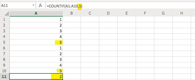
CONCAT or CONCANTENATE() Function
Similar to our example using just the ampersand ( & ) in our formula, you can combine cells using the CONCAT() function. Go ahead and try it, using our same example.
Type your first name in A1 and your last name in B1. Then, in C1 type CONCAT(A1, “ “ , B1).
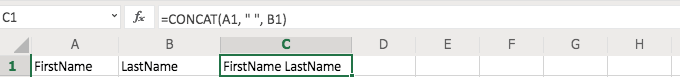
You will see that you get the same result as we did with the ampersand (&). Many people use the ampersand because it is easier and less cumbersome but now you see that you also have another option.
Note: This function may be CONCANTENATE in your version of Excel. Microsoft shortened the function name to just CONCAT and that tends to be easier to type (and remember) in the later versions of the software. Fortunately, if you start typing CONCA in your formula bar (after the equals sign), you will see which version your version of Excel uses and can select it by clicking on it with the mouse..
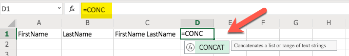
Remember that when you start to type it, to allow your version of Excel to reveal the correct function, to only type “CONCA” (or shorter) and not “CONCAN” (as the start for CONCANTENATE) or you may not see Excel’s suggestion since that is where the two functions start to differ.
Don’t be surprised if you prefer to use the merge method with the ampersand (&) instead of CONCAT(). That is normal.
If/Then Formulas
Let’s say we want to use an If/Then Formula to identify Discount (sort of a second discount) amount in a new column in our Example Excel file. In that case, first we start by adding a column and we are adding it after Column F and before Column G (again, in our downloaded example file).
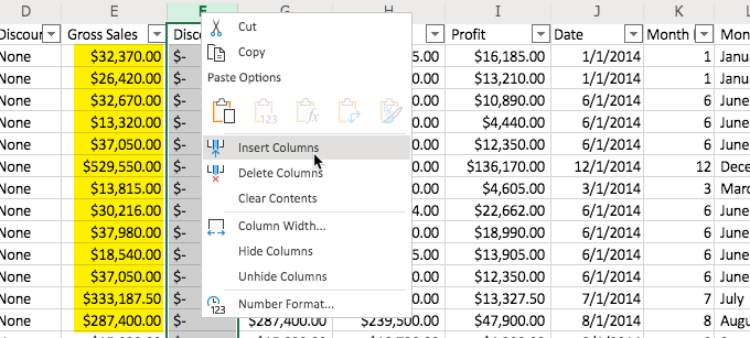
Now, we type in the formula. In this case, we type it in F2 and it is “=IF(E2>25000, “DISCOUNT 2”). This fulfills what the formula is looking for with a test (E2 greater than 25k) and then a result if the number in E2 passes that test (“DISCOUNT 2”).
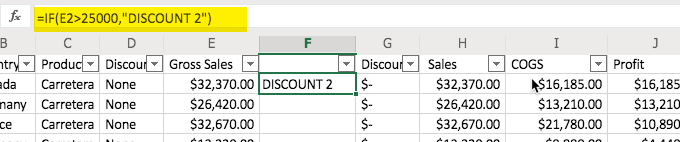
Now, copy F2 and paste in the cells that follow it in the F column.
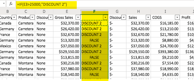
The formula will automatically adjust for each cell (relative cell referencing), with a reference to the appropriate cell. Remember that if you do not want it to automatically adjust, you can precede the cell alpha with a $ sign as well as the number, like A1 is $A$1.
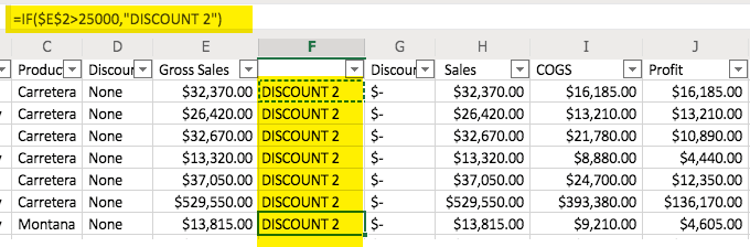
You can see, in the image above, that “DISCOUNT 2” appears in all of the cells in the F2 column. This is because the formula tells it to look at the E2 cell (represented by $E$2) and no relative cells. So, when the formula is copied to the next cell (i.e. F3) it is still looking at the E2 cell because of the dollar signs. So, all of the cells give the same result because they have the same formula referencing the same cell.
Also, if you want a value to show up instead of the word, “FALSE,” simply add a comma and then the word or number that you want to appear (text should be in quotes) at the end of the formula, before the ending parenthesis.
Pro Tip: Use VLOOKUP: Search and find a value in a different cell based on some matching text within the same row.
Managing Your Excel Projects
Fortunately, with the way that Excel documents are designed, you can do quite a bit with your Excel Workbooks. The ability to have different worksheets (tabs) in your document allows you to have related content all in one file. Also, if you feel that you are creating something that may have formulas that work better (or worse) you can copy (right-click option) your Worksheets (tabs) to have various versions of your Worksheet.
You can rename your tabs and use date codes to let you know which versions are the newest (or oldest). This is just one example of how you can use those tabs to your advantage in managing your Excel projects.
Here is an example of renaming your tabs in one of the later versions of Excel. You start by clicking on the tab and you get a result similar to the image here:
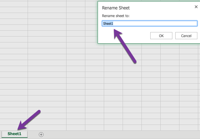
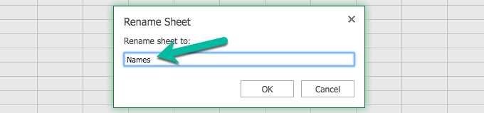
If you do not receive that response, that is ok. You may have an earlier version of Excel but it is somewhat intuitive in the way that it allows you to rename the tabs. You can right-click on the tab and get an option to “rename” in the earlier versions of Excel, as well, and sometimes simply type right in the tab.
Excel provides you with so many opportunities in your journey in learning how to use Excel. Now it is time to go out and use it! Have fun.
Перейти к содержанию
Самоучитель по Microsoft Excel для чайников
На чтение 6 мин Опубликовано 10.05.2020
Самоучитель по работе в Excel для чайников позволит Вам легко понять и усвоить базовые навыки работы в Excel, чтобы затем уверенно перейти к более сложным темам. Самоучитель научит Вас пользоваться интерфейсом Excel, применять формулы и функции для решения самых различных задач, строить графики и диаграммы, работать со сводными таблицами и многое другое.
Самоучитель был создан специально для начинающих пользователей Excel, точнее для «полных чайников». Информация дается поэтапно, начиная с самых азов. От раздела к разделу самоучителя предлагаются все более интересные и захватывающие вещи. Пройдя весь курс, Вы будете уверенно применять свои знания на практике и научитесь работать с инструментами Excel, которые позволят решить 80% всех Ваших задач. А самое главное:
- Вы навсегда забудете вопрос: «Как работать в Excel?»
- Теперь никто и никогда не посмеет назвать Вас «чайником».
- Не нужно покупать никчемные самоучители для начинающих, которые затем будут годами пылиться на полке. Покупайте только стоящую и полезную литературу!
- На нашем сайте Вы найдете еще множество самых различных курсов, уроков и пособий по работе в Microsoft Excel и не только. И все это в одном месте!
Содержание
- Раздел 1: Основы Excel
- Раздел 2: Формулы и функции
- Раздел 3: Работа с данными
- Раздел 4: Расширенные возможности Excel
- Раздел 5: Продвинутая работа с формулами в Excel
- Раздел 6: Дополнительно
- Знакомство с Excel
- Интерфейс Microsoft Excel
- Лента в Microsoft Excel
- Представление Backstage в Excel
- Панель быстрого доступа и режимы просмотра книги
- Создание и открытие рабочих книг
- Создание и открытие рабочих книг Excel
- Режим совместимости в Excel
- Сохранение книг и общий доступ
- Сохранение и автовосстановление книг в Excel
- Экспорт книг Excel
- Общий доступ к книгам Excel
- Основы работы с ячейками
- Ячейка в Excel — базовые понятия
- Содержимое ячеек в Excel
- Копирование, перемещение и удаление ячеек в Excel
- Автозаполнение ячеек в Excel
- Поиск и замена в Excel
- Изменение столбцов, строк и ячеек
- Изменение ширины столбцов и высоты строк в Excel
- Вставка и удаление строк и столбцов в Excel
- Перемещение и скрытие строк и столбцов в Excel
- Перенос текста и объединение ячеек в Excel
- Форматирование ячеек
- Настройка шрифта в Excel
- Выравнивание текста в ячейках Excel
- Границы, заливка и стили ячеек в Excel
- Числовое форматирование в Excel
- Основные сведения о листе Excel
- Переименование, вставка и удаление листа в Excel
- Копирование, перемещение и изменение цвета листа в Excel
- Группировка листов в Excel
- Разметка страницы
- Форматирование полей и ориентация страницы в Excel
- Вставка разрывов страниц, печать заголовков и колонтитулов в Excel
- Печать книг
- Панель Печать в Microsoft Excel
- Задаем область печати в Excel
- Настройка полей и масштаба при печати в Excel
Раздел 2: Формулы и функции
- Простые формулы
- Математические операторы и ссылки на ячейки в формулах Excel
- Создание простых формул в Microsoft Excel
- Редактирование формул в Excel
- Сложные формулы
- Знакомство со сложными формулами в Excel
- Создание сложных формул в Microsoft Excel
- Относительные и абсолютные ссылки
- Относительные ссылки в Excel
- Абсолютные ссылки в Excel
- Ссылки на другие листы в Excel
- Формулы и функции
- Знакомство с функциями в Excel
- Вставляем функцию в Excel
- Библиотека функций в Excel
- Мастер функций в Excel
Раздел 3: Работа с данными
- Управление внешним видом рабочего листа
- Закрепление областей в Microsoft Excel
- Разделение листов и просмотр книги Excel в разных окнах
- Сортировка данных в Excel
- Сортировка в Excel – основные сведения
- Пользовательская сортировка в Excel
- Уровни сортировки в Excel
- Фильтрация данных в Excel
- Фильтр в Excel — основные сведения
- Расширенный фильтр в Excel
- Работа с группами и подведение итогов
- Группы и промежуточные итоги в Excel
- Таблицы в Excel
- Создание, изменение и удаление таблиц в Excel
- Диаграммы и спарклайны
- Диаграммы в Excel – основные сведения
- Макет, стиль и прочие параметры диаграмм
- Как работать со спарклайнами в Excel
Раздел 4: Расширенные возможности Excel
- Работа с примечаниями и отслеживание исправлений
- Отслеживание исправлений в Excel
- Рецензирование исправлений в Excel
- Примечания к ячейкам в Excel
- Завершение и защита рабочих книг
- Завершение работы и защита рабочих книг в Excel
- Условное форматирование
- Условное форматирование в Excel
- Сводные таблицы и анализ данных
- Общие сведение о сводных таблицах в Excel
- Сведение данных, фильтры, срезы и сводные диаграммы
- Анализ «что если” в Excel
Раздел 5: Продвинутая работа с формулами в Excel
- Решаем задачи с помощью логических функций
- Как задать простое логическое условие в Excel
- Используем логические функции Excel для задания сложных условий
- Функция ЕСЛИ в Excel на простом примере
- Подсчет и суммирование в Excel
- Подсчет ячеек в Excel, используя функции СЧЕТ и СЧЕТЕСЛИ
- Суммирование в Excel, используя функции СУММ и СУММЕСЛИ
- Как посчитать накопительную сумму в Excel
- Вычисляем средневзвешенные значения при помощи СУММПРОИЗВ
- Работа с датами и временем в Excel
- Дата и время в Excel – основные понятия
- Ввод и форматирование дат и времени в Excel
- Функции для извлечения различных параметров из дат и времени в Excel
- Функции для создания и отображения дат и времени в Excel
- Функции Excel для вычисления дат и времени
- Поиск данных
- Функция ВПР в Excel на простых примерах
- Функция ПРОСМОТР в Excel на простом примере
- Функции ИНДЕКС и ПОИСКПОЗ в Excel на простых примерах
- Полезно знать
- Статистические функции Excel, которые необходимо знать
- Математические функции Excel, которые необходимо знать
- Текстовые функции Excel в примерах
- Обзор ошибок, возникающих в формулах Excel
- Работа с именами в Excel
- Знакомство с именами ячеек и диапазонов в Excel
- Как присвоить имя ячейке или диапазону в Excel
- 5 полезных правил и рекомендаций по созданию имен ячеек и диапазонов в Excel
- Диспетчер имен в Excel – инструменты и возможности
- Как присваивать имена константам в Excel?
- Работа с массивами в Excel
- Знакомство с формулами массива в Excel
- Многоячеечные формулы массива в Excel
- Одноячеечные формулы массива в Excel
- Массивы констант в Excel
- Редактирование формул массива в Excel
- Применение формул массива в Excel
- Подходы к редактированию формул массива в Excel
Раздел 6: Дополнительно
- Настройка интерфейса
- Как настроить Ленту в Excel 2013
- Режим сенсорного управления Лентой в Excel 2013
- Стили ссылок в Microsoft Excel
Хотите узнать об Excel еще больше? Специально для Вас мы припасли целых два простых и полезных самоучителя: 300 примеров по Excel и 30 функций Excel за 30 дней.
Оцените качество статьи. Нам важно ваше мнение:
Spreadsheets are a nerd’s data-driven dream. For most regular people, though, they’re a complicated mess. Fortunately, they don’t need to be. Here’s how to bend data to your will with Microsoft Excel 2016.
This post is part of Microsoft Office Week, a series at Lifehacker where we offer tips to get started with or master Microsoft Office. Want more? Be sure to keep an eye on the Office Week tag page throughout the week.
Get Up and Running With Excel Quickly
Excel is deceptively simple to get started with. The ribbon interface works exactly like the other Microsoft apps. Each tab along the top opens a new selection of menu options. If you can’t find a feature you’re looking for, explore the other tabs to find it. You can also click the green box that reads “Tell me what you want to do” to search for a menu option.
When you create a new document, you can also choose from a wide variety of templates. Excel 2016 can search thousands of online templates, including personal budgets, vacation itineraries, expense reports, inventory lists, and more. You can search the template list for keywords or browse tag pages right within the app. You can also browse Excel templates online here.
This series assumes you understand the basics, but if you need a refresher, you can check out Microsoft’s official Quick Start guides here.
How to Do the Most Common, Essential Tasks in Microsoft Excel
Spreadsheets can be as simple as a basic table and as complex as an automated role-playing game character sheet. While everyone’s needs are different, there are a few basic tasks that you can combine to make the most robust spreadsheet you need. Here’s how to do some of the most essential tasks.
How to Apply Conditional Formatting
Formatting cells in a spreadsheet can turn a boring list of numbers into a useful document that’s easy to read. You can manually set text and background colors, text size, highlights, and borders to help aid readability. The most useful feature by far, though, is the ability to style cells based on what’s in them.
For example, in the screenshot above, I have a spreadsheet of comic book movies and how much money they’ve made at the domestic and worldwide box offices (yes, I really do have this, shut up). If I want to be able to see at a glance which movies have made the most and which have made the least, I can use conditional color scales.
To apply a style, select the cells you want to apply the style to. In my case, I chose all the cells under a single column. Under the Home tab, you’ll find a button called Conditional Formatting. Click this and you’ll see a selection of styles you can apply. As you hover over each item in the menu, you’ll see a live preview so you can see how your data will appear once you make a selection. In the screenshot above, I used a style called the “Green — White — Red Color Scale.” The highest numbers are colored in green, while the lowest numbers are colored in red.
If you decide you don’t like a style or want to change it, you’ll need to clear the old style first. To do that, follow these steps:
- Click the Home tab.
- Under the Editing section, click the Clear button.
- In the drop-down menu that appears, select Clear Formats.
You can apply as many or as few styles as you want to a range of cells. You can also create your own styling rules if Excel doesn’t have the option you need built-in already. Keep in mind that a style will be applied to every cell you select, so how you choose your cells may affect how the style appears. For example, in the spreadsheet above, if I applied the style above to the domestic and global box office columns at the same time, all of the domestic values would be on the red end of the spectrum, making the style useless. In order to be useful, I needed to apply the style to each column individually.
Freeze Rows and Columns to Make Browsing Easier
The first row or column of your spreadsheet is often used for labels. In my sample spreadsheet, I want to be able to see which column I’m working out of no matter how very many superhero movies I have to scroll past. You can lock your labels in place by using the Freeze Panes feature.
Under the View tab, in the Window section, you’ll see button called Freeze Panes. If you click the drop-down menu here, you’ll find three options:
- Freeze Panes: This option will lock any rows above your cursor and any columns left of your cursor. So, for example, if you want to keep the first row and first column of your spreadsheet visible, place your cursor at cell B2 and click this button.
- Freeze Top Row: This option will freeze just the first top row in a spreadsheet.
- Freeze First Column: This option will freeze the left-most cell in a spreadsheet.
Once you’ve chosen any of these options, the first Freeze Panes option will change to Unfreeze Panes. You’ll need to unfreeze any panes before you choose new ones to lock into.
Use Formulas and Functions to Do Complex Math
All those boxes of numbers aren’t going to be very helpful if you can’t do anything with them. The formulas and functions in Excel help you do a ton of complex calculations so you can draw meaningful conclusions from your data.
Formulas are the most basic way to do math in Excel. All formulas begin with an = sign. You can then create basic problems using cell labels. For example, in the screenshot above, say I want to see how much the two standalone Wolverine films have made overall in the entire world. I would use the following formula:
=F29+F31
This would add the two numbers together—$373 + $414—to give me a grand global total of $787 million (each cell value represents millions).
Excel also has a ton of pre-made functions to do more complex math for you. For example, say you want to find out how much money the X-Men films have made globally on average in the above spreadsheet. For this, you can use the AVERAGE function. To take the average of all these films, you’d use the following line:
=AVERAGE(F26:F33)
The colon in this line indicates that the AVERAGE function should include the entire range of cells between the first and last cell. So, this function will take the average of every value for an X-Men film in column F.
You can also nest functions within each other. For example, say I want to find out the average user Rotten Tomatoes rating for each X-Men film. The average rating of all the cells in H26 through H33 in the screenshot above ends with three decimal places. Instead, I want to round that number down to a single decimal place. According to Excel’s documentation, the ROUND function should be formatted like this:
=ROUND(number, num_digits)
Here, “number” indicates the number I want to round, and “num_digits” represents the number of digits I want to round the number to. In this case, the number I want to round is the result of the AVERAGE function. So, in order to chop those extra decimal points off the average, I’ll use the following function:
=ROUND((AVERAGE(H26:H33)),1)
This is what’s called a nested function. First, Excel calculates the average of the cells in H26 through H33 (seen in bold above). Then, it uses that average as the number argument in the ROUND function. The 1 at the end of the line indicates that the number should be rounded to one decimal point. So, instead of getting an average rating of 78.875, which is the actual average rating, you see 78.9 in the final sheet.
As you can see, formulas and functions can range from very simple to incredibly complex. These examples just barely scratch the surface of what you can do with formulas and functions. You can check out this guide from the How-To Geek for a deeper dive into what you can do with functions. You can also browse the functions built into Excel and learn how to use them here.
Use Pivot Tables to Draw Meaningful Conclusions
In the above example, I used functions to manually create a table with information about my spreadsheet. Pivot tables offer an easier way to do this without having to carefully craft complex formulas to do basic tasks like rounding an average. When you’re dealing with large data sets, this can be invaluable.
You can create a pivot table in one of two ways. On the Insert tab, you can click Recommended PivotTables and Excel will suggest tables based on the data you already have entered in your spreadsheet. Alternatively, you can click PivotTable to manually create your own. Both will open the pivot table interface on a new sheet.
In a pivot table you can choose specific subsets of your data to analyze. For example, say I want to see the average Metacritic review scores. On the right side of the screen, I’ll select the Film, Metacritic, and Metacritic Users fields. This will give me the following table:
By default, the table will show me the sum of each line. While that would be handy for something like total box office gross, in this case the sum of review scores is useless. I’ll need to tweak it. To do that, I’ll click the dropdown arrow next to “Sum of Metacritic” in the Values box. Then, I’ll click Value Field Settings. This will give me new options for which data to display.
In the Summarize Values By tab, I’ll choose Average, since that’s a more meaningful calculation. Next, I’ll do the same thing for the Sum of Metacritic Users field in the Values box. This will give me a much more useful table:
Just like in the last section, that trailing decimal in the Metacritic column is bothering me. Fortunately, I don’t need to deal with nested functions this time. To fix this, I’ll open up the Value Field Settings menu again. This time, I’ll click the button at the bottom of the window that says Number Format.
In the list of categories on the left-hand side of the new window that appears, I’ll select Number. Here, I can choose how many decimal places I want to include. For the Metacritic column, I’ll choose zero, so it’s consistent with the original scoring metric. I’ll make the same change for the Metacritic Users column, but this time I’ll choose one decimal point, since Metacritic users rate on a one decimal point scale. My new table is much cleaner:
My new pivot table is much easier to read. You can use pivot tables to examine your data in a variety of ways without changing the sheet your data is stored on. For example, I can quickly add columns for Box Office data or Rotten Tomatoes ratings. I could also drag the Film field from the Rows box to the Filters box so that my table only displays the totals for each column, instead of the individual lines themselves.
When you’re dealing with huge data sets, pivot tables become essential. Sometimes they can be a bit difficult if your data isn’t formatted quite right (the blank rows I leave between different franchises regularly throws off automatic pivot tables, for example), but they’re often much quicker and more flexible than building your own tables from formulas.
Insert Page Breaks to Make Printing Spreadsheets Easy
Unlike Word documents, spreadsheets aren’t designed with regular, easy-to-print pages in mind. To compensate for this, use the Page Break Preview feature. With it, you can change how your sheet is divided and what data should print on which page.
To open this view, click the View tab. In the Workbook View section, click Page Break Preview. Your spreadsheet will zoom out and show you which sections will print on each page. You can drag each line to resize the sections as you see fit.
If you want to add more page breaks, follow these steps:
- Place your cursor on the row or column where you want to create a new page break.
- Click the Page Layout tab on the ribbon interface.
- Click the Breaks button.
- In the dropdown that pops up, click Insert Page Break.
In the case of very long documents, Excel may introduce automatic page breaks when you reach the maximum amount of space that can fit on a page. You can’t remove these page breaks, but any of the others including the page breaks you add can be moved or removed at will. To get back to the normal view, return to the View tab in the ribbon. Under Workbook Views, click Normal.
Create Charts to Visualize Your Data
To get a better idea of what your data looks like, you can create custom charts based on all or part of the data in your spreadsheet. Excel comes with a ton of ready-made styles you can choose from, or you can customize your charts to suit your needs.
To create a chart, first select the cells you want to include. In some cases, you may need to format your cells a certain way for Excel to understand them, but you can read about how to format your cells for each type of chart here. In this example, we’ll use the movie data for the Marvel Cinematic Universe in the screenshot above. I’ll select everything in columns A, E, and F.
Once you’ve selected your data, click the Insert tab in the ribbon. In the Charts section, you’ll see a button called Recommended Charts. This will automatically choose the type of chart that Excel thinks is best based on the data you’ve selected. In my case, I chose “clustered columns” from my suggestions.
Once you’ve created your chart, you can customize it how you need. In my case, there are a few things I don’t like about this one. I want to change the chart title so it’s more descriptive. I want to add a label to the left axis to indicate that the numbers are measured in millions. Also, it would be nice if the color scheme was a little bit less boring.
The first problem is easy. You can click the title of a chart to change it. To change the axis labels, you’ll need to add one first. Click somewhere in the empty space on the chart to select the chart itself. Three buttons will appear next to the top right corner of the chart. Click the first button with a green plus icon. Here, you can add elements like an axis title. You can then click the label to edit it the same way you edited the title.
To change the style of the chart, select it and click the box with a paintbrush symbol on it. Here, you can choose from a selection of preset styles. You can also change the color scheme of your chart by clicking Color at the top of the style-picker box. Now, doesn’t this chart look so much nicer?
By default, any new charts you create will appear on the sheet you have open. If you’d rather keep your charts separate, you can move them to their own sheet. To do so, right-click the chart and select Move Chart. In the box that appears, select “New sheet” and give it a name. Click OK and the chart will be moved to its own sheet.
The Best New Features of Excel 2016
The basics of spreadsheets are as fundamental as math itself. Even so, Microsoft has managed to add new useful features in Excel 2016. Here are some of the best tools in the most recent version:
- You can search the ribbon: Just like the other new Microsoft Office apps, you can search the ribbon if you can’t find the feature you’re looking for. Click the green box at the top of the screen that says “Tell me what you want to do.” Enter keywords or describe what you want to do and Excel will suggest features for you.
- Collaborate with others in real-time: Another feature common to all Office apps, you can share your documents to your OneDrive account and work with other users on the same document at the same time. Much like Google Docs, everyone can see each other’s changes as they happen.
- Research in the app with Smart Lookup: If you need to find some quick information on a cell in your document, you can use the Smart Lookup tool to find it without having to leave the app. You can get links to Wikipedia, definitions of words, and get Bing image search results all inside Excel.
- Draw your formulas with Ink Equations: Some math equations are easier to write than they are to type. In Excel 2016, you can draw math equations to add them into your spreadsheet. This is particularly handy if you have a stylus or touchscreen on your computer.
There’s a lot more buried old and new features buried underneath the surface. You can check out more about the newest versions on Microsoft’s website.
Work Faster in Excel With These Keyboard Shortcuts
You can find a complete list of keyboard shortcuts for nearly everything in Excel on Microsoft’s website here. Here are some of the most common ones that you’ll use every day:
- Ctrl+N/Ctrl+O/Ctrl+S: Create, Open, and Save a document.
- Ctrl+X/Ctrl+C/Ctrl+V: Cut, Copy, Paste
- Ctrl+B/Ctrl+I: Bold, Italic
- Ctrl+Page Up/Page Down: Next/previous sheet
- Ctrl+F1: Expand or collapse the ribbon
- Alt+H: Go to the Home tab on the ribbon.
- Ctrl+Arrows: Move to edge of section
- Shift+Space: Select entire row
- Ctrl+Space: Select entire column
- Ctrl+;: Enter current date.
- Ctrl+Alt+;: Enter current time.
Excel also supports many of the same text navigation shortcuts that we’ve covered previously here. You can also navigate the ribbon by pressing Alt. The app will then show you what button you can press to change tabs or access the functions currently available.
Additional Reading for Power Users
There’s virtually no limit to the ways you can use Excel to make your own spreadsheets. You can create anything from a simple to-do list to sheets that damn near seem like applications of their own. Here’s some more reading to help you on your way:
- Four skills that will turn you into a spreadsheet ninja: Mastering spreadsheets is an art. Our guide here will teach you about input forms, statistical calculations, pivot tables, and macros.
- Learn how to master VLOOKUP to find data easily: One of the most useful functions in Excel is called VLOOKUP. This allows you to lookup one piece of data in your spreadsheet based on another piece of data you already know. For example, if you have a document that lists the name, price, and SKU of a product, you can create a formula that finds the price when you enter a name or a SKU.
- Download free Excel templates to manage time, money or productivity: There’s no need to reinvent the wheel. Not only does Excel have a huge repository of spreadsheet templates built-in, but you can find plenty more online to suit your needs. Find one you like before you try to build your own from scratch.
- Excel Formulas: Why do you need formulas and functions?: This collection of guides from the How-To Geek covers intermediate to advanced lessons on how to use Excel functions and create formulas of your own.
Spreadsheets aren’t nearly as boring as the movies have led you to believe. While it can take a little work to get started, you can turn tediously collected data into visually impressive and informative charts.
Microsoft Excel know-how is so expected that it hardly warrants a line on a resume anymore. But how well do you really know how to use it?
Marketing is more data-driven than ever before. At any time you could be tracking growth rates, content analysis, or marketing ROI. You may know how to plug in numbers and add up cells in a column in Excel, but that’s not going to get you far when it comes to metrics reporting.
![Download 10 Excel Templates for Marketers [Free Kit]](https://no-cache.hubspot.com/cta/default/53/9ff7a4fe-5293-496c-acca-566bc6e73f42.png)
Do you want to understand what pivot tables are? Are you ready for your first VLOOKUP? Aspiring Excel wizard, read on or jump to the section that interests you most:
What is Microsoft Excel?
Microsoft Excel is a popular spreadsheet software program for business. It’s used for data entry and management, charts and graphs, and project management. You can format, organize, visualize, and calculate data with this tool.
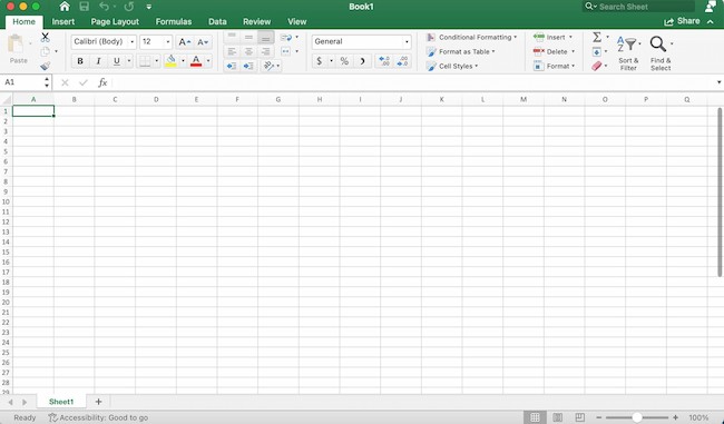
How to Download Microsoft Excel
It’s easy to download Microsoft Excel. First, check to make sure that your PC or Mac meets Microsoft’s system requirements. Next, sign in and install Microsoft 365.
After you sign in, follow the steps for your account and computer system to download and launch the program.
For example, say you’re working on a Mac desktop. You’ll click on Launchpad or look in your applications folder. Then, click on the Excel icon to open the application.
Microsoft Excel Spreadsheet Basics
Sometimes, Excel seems too good to be true. Need to combine data in multiple cells? Excel can do it. Need to copy formatting across an array of cells? Excel can do that, too.
Let’s start this Excel guide with the basics. Once you have these functions down, you’ll be ready to tackle more pro Excel tips and advanced lessons.
Inserting Rows or Columns
As you work with data, you might find yourself needing to add more rows and columns. Doing this one at a time would be super tedious. Luckily, there’s an easier way.
To add multiple rows or columns in a spreadsheet, highlight the number of pre-existing rows or columns that you want to add. Then, right-click and select «Insert.»
In this example, I add three rows to the top of my spreadsheet.
Autofill
Autofill lets you quickly fill adjacent cells with several types of data, including values, series, and formulas.
There are many ways to deploy this feature, but the fill handle is among the easiest.
First, choose the cells you want to be the source. Next, find the fill handle in the lower-right corner of the cell. Then either drag the fill handle to cover the cells you want to fill or just double-click.
Filters
When you’re looking at large data sets, you usually don’t need to look at every row at the same time. Sometimes, you only want to look at data that fit into certain criteria. That’s where filters come in.
Filters allow you to pare down data to only see certain rows at one time. In Excel, you can add a filter to each column in your data. From there, you can choose which cells you want to view.
To add a filter, click the Data tab and select «Filter.» Next, click the arrow next to the column headers. This lets you choose whether you want to organize your data in ascending or descending order, as well as which rows you want to show.
Let’s take a look at the Harry Potter example below. Say you only want to see the students in Gryffindor. By selecting the Gryffindor filter, the other rows disappear.
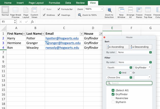
Pro tip: Start with a filtered view in your original spreadsheet. Then, copy and paste the values to another spreadsheet before you start analyzing.
Sort
Sometimes you’ll have a disorganized list of data. This is typical when you’re exporting lists, like marketing contacts or blog posts. Excel’s sort feature can help you alphabetize any list.
Click on the data in the column you want to sort. Then click on the «Data» tab in your toolbar and look for the «Sort» option on the left.
- If the «A» is on top of the «Z,» you can just click on that button once. Choosing A-Z means the list will sort in alphabetical order.
- If the «Z» is on top of the «A,» click the button twice. Z-A selection means the list will sort in reverse alphabetical order.
Remove Duplicates
Large datasets tend to have duplicate content. For example, you may have a list of different company contacts, but you only want to see the number of companies you have. In situations like this, removing duplicates comes in handy.
To remove duplicates, highlight the row or column where you noticed duplicate data. Then, go to the Data tab, and select «Remove Duplicates» (under Tools). A pop-up will appear so that you can confirm which data you want to keep. Select «Remove Duplicates,» and you’re good to go.
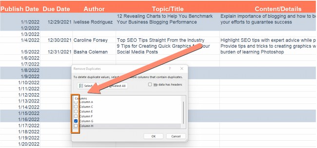
If you want to see an example, this post offers step-by-step instructions for removing duplicates.
You can also use this feature to remove an entire row based on a duplicate column value. So, say you have three rows of information and you only need to see one, you can select the whole dataset and then remove duplicates. The resulting list will have only unique data without any duplicates.
Paste Special
It’s often helpful to change the items in a row of data into a column (or vice versa). It would take a lot of time to copy and paste each individual header.
Not to mention, you may easily fall into one of the biggest, most unfortunate Excel traps — human error. Read here to check out some of the most common Microsoft Excel errors.
Instead of making one of these errors, let Excel do the work for you. Take a look at this example:
To use this function, highlight the column or row you want to transpose. Then, right-click and select «Copy.»
Next, select the cells where you want the first row or column to begin. Right-click on the cell, and then select «Paste Special.»
When the module appears, choose the option to transpose.
Paste Special is a super useful function. In the module, you can also choose between copying formulas, values, formats, or even column widths. This is especially helpful when it comes to copying the results of your pivot table into a chart.
Text to Columns
What if you want to split out information that’s in one cell into two different cells? For example, maybe you want to pull out someone’s company name through their email address. Or you want to separate someone’s full name into a first and last name for your email marketing templates.
Thanks to Microsoft Excel, both are possible. First, highlight the column where you want to split up. Next, go to the Data tab and select «Text to Columns.» A module will appear with more information. First, you need to select either «Delimited» or «Fixed Width.»
- Delimited means you want to break up the column based on characters such as commas, spaces, or tabs.
- Fixed Width means you want to select the exact location in all the columns where you want the split to occur.
Select «Delimited» to separate the full name into first name and last name.
Then, it’s time to choose the delimiters. This could be a tab, semicolon, comma, space, or something else. (For example, «something else» could be the «@» sign used in an email address.) Let’s choose the space for this example. Excel will then show you a preview of what your new columns will look like.
When you’re happy with the preview, press «Next.» This page will allow you to select Advanced Formats if you choose to. When you’re done, click «Finish.»
Format Painter
Excel has a lot of features to make crunching numbers and analyzing your data quick and easy. But if you ever spent some time formatting a spreadsheet, you know it can get a bit tedious.
Don’t waste time repeating the same formatting commands over and over again. Use the format painter to copy formatting from one area of the worksheet to another.
To do this, choose the cell you’d like to replicate. Then, select the format painter option (paintbrush icon) from the top toolbar. When you release the mouse, your cell should show the new format.
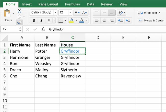
Keyboard Shortcuts
Creating reports in Excel is time-consuming enough. How can we spend less time navigating, formatting, and selecting items in our spreadsheet? Glad you asked. There are a ton of Excel shortcuts out there, including some of our favorites listed below.
Create a New Workbook
PC: Ctrl-N | Mac: Command-N
Select Entire Row
PC: Shift-Space | Mac: Shift-Space
Select Entire Column
PC: Ctrl-Space | Mac: Control-Space
Select Rest of Column
PC: Ctrl-Shift-Down/Up | Mac: Command-Shift-Down/Up
Select Rest of Row
PC: Ctrl-Shift-Right/Left | Mac: Command-Shift-Right/Left
Add Hyperlink
PC: Ctrl-K | Mac: Command-K
Open Format Cells Window
PC: Ctrl-1 | Mac: Command-1
Autosum Selected Cells
PC: Alt-= | Mac: Command-Shift-T
Excel Formulas
At this point, you’re getting used to Excel’s interface and flying through quick commands on your spreadsheets.
Now, let’s dig into the core use case for the software: Excel formulas. Excel can help you do simple arithmetic like adding, subtracting, multiplying, or dividing any data.
- To add, use the + sign.
- To subtract, use the — sign.
- To multiply, use the * sign.
- To divide, use the / sign.
- To use exponents, use the ^ sign.
Remember, all formulas in Excel must begin with an equal sign (=). Use parentheses to make sure certain calculations happen first. For example, consider how =10+10*10 is different from =(10+10)*10.
Besides manually typing in simple calculations, you can also refer to Excel’s built-in formulas. Some of the most common include:
- Average: =AVERAGE(cell range)
- Sum: =SUM(cell range)
- Count: =COUNT(cell range)
Also note that series’ of specific cells are separated by a comma (,), while cell ranges are notated with a colon (:). For example, you could use any of these formulas:
- =SUM(4,4)
- =SUM(A4,B4)
- =SUM(A4:B4)
Conditional Formatting
Conditional formatting lets you change a cell’s color based on the information within the cell. For example, say you want to flag a category in your spreadsheet.
To get started, highlight the group of cells you want to use conditional formatting on. Then, choose «Conditional Formatting» from the Home menu. Next, select a logic option from the dropdown. A window will pop up that prompts you to provide more information about your formatting rule. Select «OK» when you’re done, and you should see your results automatically appear.
Note: You can also create your own logic if you want something beyond the dropdown choices.
Dollar Signs
Have you ever seen a dollar sign in an Excel formula? When this symbol is in a formula, it isn’t representing an American dollar. Instead, it makes sure that the exact column and row stay the same even if you copy the same formula in adjacent rows.
You see, a cell reference — when you refer to cell A5 from cell C5, for example — is relative by default.
This means you’re actually referring to a cell that’s five columns to the left (C minus A) and in the same row (5). This is called a relative formula.
When you copy a relative formula from one cell to another, it’ll adjust the values in the formula based on where it’s moved. But sometimes, you want those values to stay the same no matter whether they’re moved around or not. You can do that by making the formula in the cell into what’s called an absolute formula.
To change the relative formula (=A5+C5) into an absolute formula, precede the row and column values with dollar signs, like this: (=$A$5+$C$5).
Combine Cells Using «&»
Databases tend to split out data to make it as exact as possible. For example, instead of having data that shows a person’s full name, a database might have the data as a first name and then a last name in separate columns.
In Excel, you can combine cells with different data into one cell by using the «&» sign in your function. The example below uses this formula: =A2&» «&B2.
Let’s go through the formula together using an example. So, let’s combine first names and last names into full names in a single column.
To do this, put your cursor in the blank cell where you want the full name to appear. Next, highlight one cell that contains a first name, type in an «&» sign, and then highlight a cell with the corresponding last name.
But you’re not finished. If all you type in is =A2&B2, then there will not be a space between the person’s first name and last name. To add that necessary space, use the function =A2&» «&B2. The quotation marks around the space tell Excel to put a space between the first and last name.
To make this true for multiple rows, drag the corner of that first cell downward as shown in the example.
Pivot Tables
Pivot tables reorganize data in a spreadsheet. A pivot table won’t change the data that you have, but it can sum up values and compare information in a way that’s easy to understand.
For example, let’s look at how many people are in each house at Hogwarts.
To create the Pivot Table, go to Insert > Pivot Table. Excel will automatically populate your pivot table, but you can always change the order of the data. Then, you have four options to choose from.
Report Filter
This allows you to only look at certain rows in your dataset.
For example, to create a filter by house, choose only students in Gryffindor.
Column and Row Labels
These could be any headers or rows in the dataset.
Note: Both Row and Column labels can contain data from your columns. For example, you can drag First Name to either the Row or Column label depending on how you want to see the data.
Value
This section allows you to convert data into a number. Instead of just pulling in any numeric value, you can sum, count, average, max, min, count numbers, or do a few other manipulations with your data. By default, when you drag a field to Value, it always does a count.
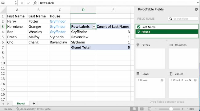
The example above counts the number of students in each house. To recreate this pivot table, go to the pivot table and drag the House column to both the row Labels and the values. This will sum up the number of students associated with each house.
IF Functions
At its most basic level, Excel’s IF function lets you see if a condition you set is true or false for a given value.
If the condition is true, you get one result. If the condition is false, you get another result.
This popular tool is useful for comparisons and finding errors. But if you’re new to Excel you may need a little more information to get the most out of this feature.
Let’s take a look at this function’s syntax:
- =IF(logical_test, value_if_true, [value_if_false])
- With values, this could be: =IF(A2>B2, «Over Budget», «OK»)
In this example, you want to find where you’re overspending. With this IF function, if your spending (what’s in A2) is greater than your budget (what’s in B2), that overspending will be easy to see. Then you can then filter the data so that you see only the line items where you’re going over budget.
The real power of the IF function comes when you string or «nest» multiple IF statements together. This allows you to set multiple conditions, get more specific results, and organize your data into more manageable chunks.
For example, ranges are one way to segment your data for better analysis. For example, you can categorize data into values that are less than 10, 11 to 50, or 51 to 100.
- =IF(B3<11,»10 or less»,IF(B3<51,»11 to 50″,IF(B3<100,»51 to 100″)))
Let’s talk about a few more IF functions.
COUNTIF Function
The power of IF functions goes beyond simple true and false statements. With the COUNTIF function, Excel can count the number of times a word or number appears in any range of cells.
For example, let’s say you want to count the number of times the word «Gryffindor» appears in this data set.
Take a look at the syntax.
- The formula: =COUNTIF(range, criteria)
- The formula with variables from the example below: =COUNTIF(D:D,»Gryffindor»)
In this formula, there are several variables:
Range
The range that you want the formula to cover.
In this one-column example, «D:D» shows that the first and last columns are both D. If you want to look at columns C and D, use «C:D.»
Criteria
Whatever number or piece of text you want Excel to count.
Only use quotation marks if you want the result to be text instead of a number. In this example, «Gryffindor» is the only criteria.
To use this function, type the COUNTIF formula in any cell and press «Enter.» Using the example above, this action will show how many times the word «Gryffindor» appears in the dataset.
SUMIF Function
Ready to make the IF function a bit more complex? Let’s say you want to analyze the number of leads your blog has generated from one author, not the entire team.
With the SUMIFS function, you can add up cells that meet certain criteria. You can add as many different criteria to the formula as you like.
Here’s your formula:
- =SUMIFS(sum_range, criteria_range1, criteria1, [criteria_range2, criteria 2],etc.)
That’s a lot of criteria. Let’s take a look at each part:
Sum_range
The range of cells you’re going to add up.
Criteria_range1
The range that is being searched for your first value.
Criteria1
This is the specific value that determines which cells in Criteria_range1 to add together.
Note: Remember to use quotation marks if you’re searching for text.
In the example below, the SUMIF formula counts the total number of house points from Gryffindor.

If AND/OR
The OR and AND functions round out your IF function choices. These functions check multiple arguments. It returns either TRUE or FALSE depending on if at least one of the arguments is true (this is the OR function), or if all of them are true (this is the AND function).
Lost in a sea of «and’s» and «or’s»? Don’t check out yet. In practice, OR and AND functions will never be used on their own. They need to be nested inside of another IF function. Recall the syntax of a basic IF function:
- =IF(logical_test, value_if_true, [value_if_false])
- Now, let’s fit an OR function inside of the logical_test: =IF(OR(logical1, logical2), value_if_true, [value_if_false])
To put it plainly, this combined formula allows you to return a value if both conditions are true, as opposed to just one. With AND/OR functions, your formulas can be as simple or complex as you want them to be, as long as you understand the basics of the IF function.
VLOOKUP
Have you ever had two sets of data on two different spreadsheets that you want to combine into a single spreadsheet?
For example, say you have a list of names and email addresses in one spreadsheet and a list of email addresses and company names in a different spreadsheet. But you want the names, email addresses, and company names of those people to appear in one spreadsheet.
VLOOKUP is a great go-to formula for this.
Before you use the formula, be sure that you have at least one column that appears identically in both places.
Note: Scour your data sets to make sure the column of data you’re using to combine spreadsheets is exactly the same. This includes removing any extra spaces.
In the example below, Sheet One and Sheet Two are both lists with different information about the same people. The common thread between the two is their email addresses. Let’s combine both datasets so that all the house information from Sheet Two translates over to Sheet One.
Type in the formula: =VLOOKUP(C2,Sheet2!A:B,2,FALSE). This will bring all the house data into Sheet One.
Now that you’ve seen how VLOOKUP works, let’s review the formula.
- The formula: =VLOOKUP(lookup value, table array, column number, [range lookup])
- The formula with variables from the example: =VLOOKUP(C2,Sheet2!A:B,2,FALSE)
In this formula, there are several variables.
Lookup Value
A value that LOOKUP searches for in an array. So, your lookup value is the identical value you have in both spreadsheets.
In the example, the lookup value is the first email address on the list, or cell 2 (C2).
Table Array
Table arrays hold column-oriented or tabular data, like the columns on Sheet Two you’re going to pull your data from.
This table array includes the column of data identical to your lookup value in Sheet One and the column of data you’re trying to copy to Sheet Two.
In the example, «A» means Column A in Sheet Two. The «B» means Column B.
So, the table array is «Sheet2!A:B.»
Column Number
Excel refers to columns as letters and rows as numbers. So, the column number is the selected column for the new data you want to copy.
In the example, this would be the «House» column. «House» is column 2 in the table array.
Note: Your range can be more than two columns. For example, if there are three columns on Sheet Two — Email, Age, and House — and you also want to bring House onto Sheet One, you can still use a VLOOKUP. You just need to change the «2» to a «3» so it pulls back the value in the third column. The formula for this would be: =VLOOKUP(C2:Sheet2!A:C,3,false).]
Range Lookup
This term means that you’re looking for a value within a range of values. You can also use the term «FALSE» to pull only exact value matches.
Note: VLOOKUP will only pull back values to the right of the column containing your identical data on the second sheet. This is why some people prefer to use the INDEX and MATCH functions instead.
INDEX MATCH
Like VLOOKUP, the INDEX and MATCH functions pull data from another dataset into one central location. Here are the main differences:
VLOOKUP is a much simpler formula.
If you’re working with large datasets that need thousands of lookups, the INDEX MATCH function will decrease load time in Excel.
INDEX MATCH formulas work right-to-left.
VLOOKUP formulas only work as a left-to-right lookup. So, if you need to do a lookup that has a column to the right of the results column, you’d have to rearrange those columns to do a VLOOKUP. This can be tedious with large datasets and lead to errors.
Let’s look at an example. Let’s say Sheet One contains a list of names and their Hogwarts email addresses. Sheet Two contains a list of email addresses and each student’s Patronus.
The information that lives in both sheets is the email addresses column. But, the column numbers for email addresses are different on the two sheets. So, you’d use the INDEX MATCH formula instead of VLOOKUP to avoid column-switching errors.
The INDEX MATCH formula is the MATCH formula nested inside the INDEX formula.
- The formula: =INDEX(table array, MATCH formula)
- This becomes: =INDEX(table array, MATCH (lookup_value, lookup_array))
- The formula with variables from the example: =INDEX(Sheet2!A:A,(MATCH(Sheet1!C:C,Sheet2!C:C,0)))
Here are the variables:
Table Array
The range of columns on Sheet Two that contain the new data you want to bring over to Sheet One.
In the example, «A» means Column A, and has the «Patronus» information for each person.
Lookup Value
This Sheet One column has identical values in both spreadsheets.
In the example, this is the «email» column on Sheet One, which is Column C. So, Sheet1!C:C.
Lookup Array
Again, an array is a group of values in rows and columns that you want to search.
In this example, the lookup array is the column in Sheet Two that contains identical values in both spreadsheets. So, the «email» column on Sheet Two, Sheet2!C:C.
Once you have your variables set, type in the INDEX MATCH formula. Add it where you want the combined information to populate.
Data Visualization
Now that you’ve learned formulas and functions, let’s make your analysis visual. With a beautiful graph, your audience will be able to process and remember your data more easily.
Create a Basic Graph
First, decide what type of graph to use. Bar charts and pie charts help you compare categories. Pie charts compare part of a whole and are often best when one of the categories is way larger than the others. Bar charts highlight incremental differences between categories. Finally, line charts can help display trends over time.
This post can help you find the best chart or graph for your presentation.
Next, highlight the data you want to turn into a chart. Then choose «Charts» in the top navigation. You can also use Insert > Chart if you have an older version of Excel. Then you can adjust and resize your chart until it makes the statement you’re hoping for.
Microsoft Excel Can Help Your Business Grow
Excel is a useful tool for any small business. Whether you’re focused on marketing, HR, sales, or service, these Microsoft Excel tips can boost your performance.
Whether you want to improve efficiency or productivity, Excel can help. You can find new trends and organize your data into usable insights. It can make your data analysis easier to understand and your daily tasks easier.
All it takes is a little know-how and some time with the software. So start learning, and get ready to grow.
Editor’s note: This post was originally published in April 2018 and has been updated for comprehensiveness.
