
Use Excel as your calculator
Instead of using a calculator, use Microsoft Excel to do the math!
You can enter simple formulas to add, divide, multiply, and subtract two or more numeric values. Or use the AutoSum feature to quickly total a series of values without entering them manually in a formula. After you create a formula, you can copy it into adjacent cells — no need to create the same formula over and over again.
Subtract in Excel

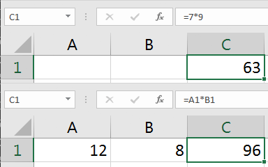
Multiply in Excel
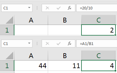
Divide in Excel
Learn more about simple formulas
All formula entries begin with an equal sign (=). For simple formulas, simply type the equal sign followed by the numeric values that you want to calculate and the math operators that you want to use — the plus sign (+) to add, the minus sign (—) to subtract, the asterisk (*) to multiply, and the forward slash (/) to divide. Then, press ENTER, and Excel instantly calculates and displays the result of the formula.
For example, when you type =12.99+16.99 in cell C5 and press ENTER, Excel calculates the result and displays 29.98 in that cell.
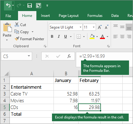
The formula that you enter in a cell remains visible in the formula bar, and you can see it whenever that cell is selected.
Important: Although there is a SUM function, there is no SUBTRACT function. Instead, use the minus (-) operator in a formula; for example, =8-3+2-4+12. Or, you can use a minus sign to convert a number to its negative value in the SUM function; for example, the formula =SUM(12,5,-3,8,-4) uses the SUM function to add 12, 5, subtract 3, add 8, and subtract 4, in that order.
Use AutoSum
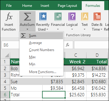
The easiest way to add a SUM formula to your worksheet is to use AutoSum. Select an empty cell directly above or below the range that you want to sum, and on the Home or Formula tabs of the ribbon, click AutoSum > Sum. AutoSum will automatically sense the range to be summed and build the formula for you. This also works horizontally if you select a cell to the left or right of the range that you need to sum.
Note: AutoSum does not work on non-contiguous ranges.
AutoSum vertically
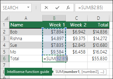
In the figure above, the AutoSum feature is seen to automatically detect cells B2:B5 as the range to sum. All you need to do is press ENTER to confirm it. If you need to add/exclude more cells, you can hold the Shift Key + the arrow key of your choice until your selection matches what you want. Then press Enter to complete the task.
Intellisense function guide: the SUM(number1,[number2], …) floating tag beneath the function is its Intellisense guide. If you click the SUM or function name, it will change o a blue hyperlink to the Help topic for that function. If you click the individual function elements, their representative pieces in the formula will be highlighted. In this case, only B2:B5 would be highlighted, since there is only one number reference in this formula. The Intellisense tag will appear for any function.
AutoSum horizontally

Learn more in the article on the SUM function.
Avoid rewriting the same formula
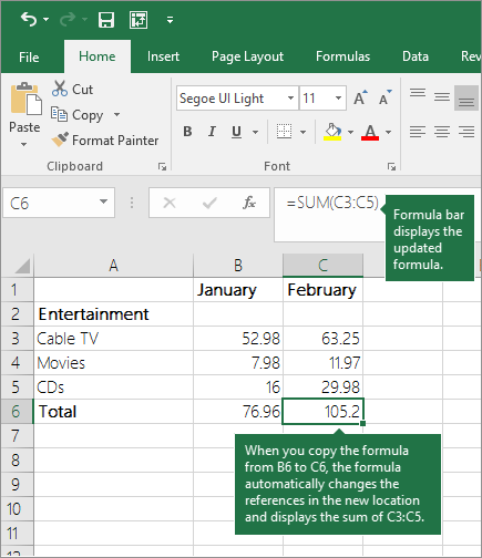
After you create a formula, you can copy it to other cells — no need to rewrite the same formula. You can either copy the formula, or use the fill handle  to copy the formula to adjacent cells.
For example, when you copy the formula in cell B6 to C6, the formula in that cell automatically changes to update to cell references in column C.
When you copy the formula, ensure that the cell references are correct. Cell references may change if they have relative references. For more information, see Copy and paste a formula to another cell or worksheet.
What can I use in a formula to mimic calculator keys?
|
Calculator key |
Excel method |
Description, example |
Result |
|
+ (Plus key) |
+ (plus) |
Use in a formula to add numbers. Example: =4+6+2 |
12 |
|
— (Minus key) |
— (minus) |
Use in a formula to subtract numbers or to signify a negative number. Example: =18-12 Example: =24*-5 (24 times negative 5) |
-120 |
|
x (Multiply key) |
* (asterisk; also called «star») |
Use in a formula to multiply numbers. Example: =8*3 |
24 |
|
÷ (Divide key) |
/ (forward slash) |
Use in a formula to divide one number by another. Example: =45/5 |
9 |
|
% (Percent key) |
% (percent) |
Use in a formula with * to multiply by a percent. Example: =15%*20 |
3 |
|
√ (square root) |
SQRT (function) |
Use the SQRT function in a formula to find the square root of a number. Example: =SQRT(64) |
8 |
|
1/x (reciprocal) |
=1/n |
Use =1/n in a formula, where n is the number you want to divide 1 by. Example: =1/8 |
0.125 |
Need more help?
You can always ask an expert in the Excel Tech Community or get support in the Answers community.
Need more help?
It’s hard to get excited about learning math. It’s something that most of us spend our lives avoiding. It’s also one of the best reasons to use Microsoft Excel for perfect calculations, every time.
Don’t think of these Excel formulas as math for math’s sake. Instead, imagine how these formulas can help you automate your life and skip the trouble of making manual calculations. At the end of this tutorial, you’ll have the skills you need to do all of the following, for example:
- Calculate the average score of your exams.
- Quickly subtotal the invoices you’ve issued to clients.
- Use basic statistics to review a set of data for trends and indicators.
You don’t have to be an accountant to master math in Excel, however. To follow along with this tutorial, make sure to download the example Excel workbook here or click on the blue Download Attachment button on the right side of this tutorial—in either case it’s free to use.
The Excel workbook has comments and instructions for how to use these formulas. As you follow along in this tutorial, I’ll teach you some of the essential «math» skills. Let’s get started.
Basic Excel Math Formulas Video (Watch and Learn)
If learning from a screencast video is your style, check out the video below to walk through the tutorial. Otherwise, keep reading for a detailed description of how to work with each Excel math formula.
Formula Basics
Before we get started, let’s look at how to use any formula in Microsoft Excel. Whether you’re working with the math formulas in this tutorial or any others, these tips will help you master Excel.
1. Each Formula in Excel Starts with «=»
To type a formula, click in any cell in Microsoft Excel and type the equals sign on your keyboard. This starts a formula.


After the equals sign, you can put an incredible variety of things into the cell. Try typing =4+4 as your very first formula, and press enter to return the result. Excel will output 8, but the formula is still behind the scenes in the spreadsheet.
2. Formulas are Shown in Excel’s Formula Bar
When you’re typing a formula into a cell, you can see the results of the cell once you press enter. But when you select a cell, you can see the formula for that cell in the formula bar.


To use the example from above, the cell will show «8» , but when we click on that cell, the formula bar will show that the cell is adding 4 and 4.
3. How to Build a Formula
In the example above, we typed a simple addition formula to add two numbers. But, you don’t have to type numbers, you can also reference other cells.
Excel is a grid of cells, with the columns running left to right, each assigned a letter, while the rows are numbered. Each cell is an intersection of a row and a column. The cell where column A and row 3 intersect is called A3, for example.


Let’s say that I have two cells with simple numbers, like 1 and 2, and they are in cells A2 and A3. When I type a formula, I can start the formula with «=» as always. Then, I can type:
=A2+A3
…to add those two numbers together. It’s very common to have a sheet with values, and then a separate sheet where calculations are performed. Keep all of these tips in mind while working with this tutorial. For each of the formulas, you can reference cells, or directly type numerical values into the formula.
If you need to change a formula that you’ve already typed, double click on the cell. You’ll be able to adjust the values in the formula.
Arithmetic in Excel
Now we’ll cover Excel math formulas and walk through how to use them. Let’s start off by exploring the basic arithmetic formula. These are the foundation of math operations.
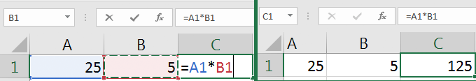
1. Add and Subtract
Addition and subtraction are two essential math formulas in Excel. Whether you’re adding up your list of business expenses for the month or balancing your checkbook digitally, the addition and subtraction operators are incredibly useful.
Use the tab titled «Add and Subtract» in the workbook for practice.
Add Values
Example:
=24+48
or, reference values in cells with:
=A2+A3
Tip: try adding five or six values to see what happens. Separate each item with a plus sign.
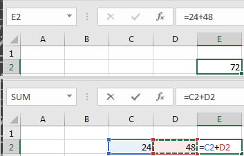
Subtract Values
Example:
=75-25-10
or, reference values in cells with:
=A3-A2
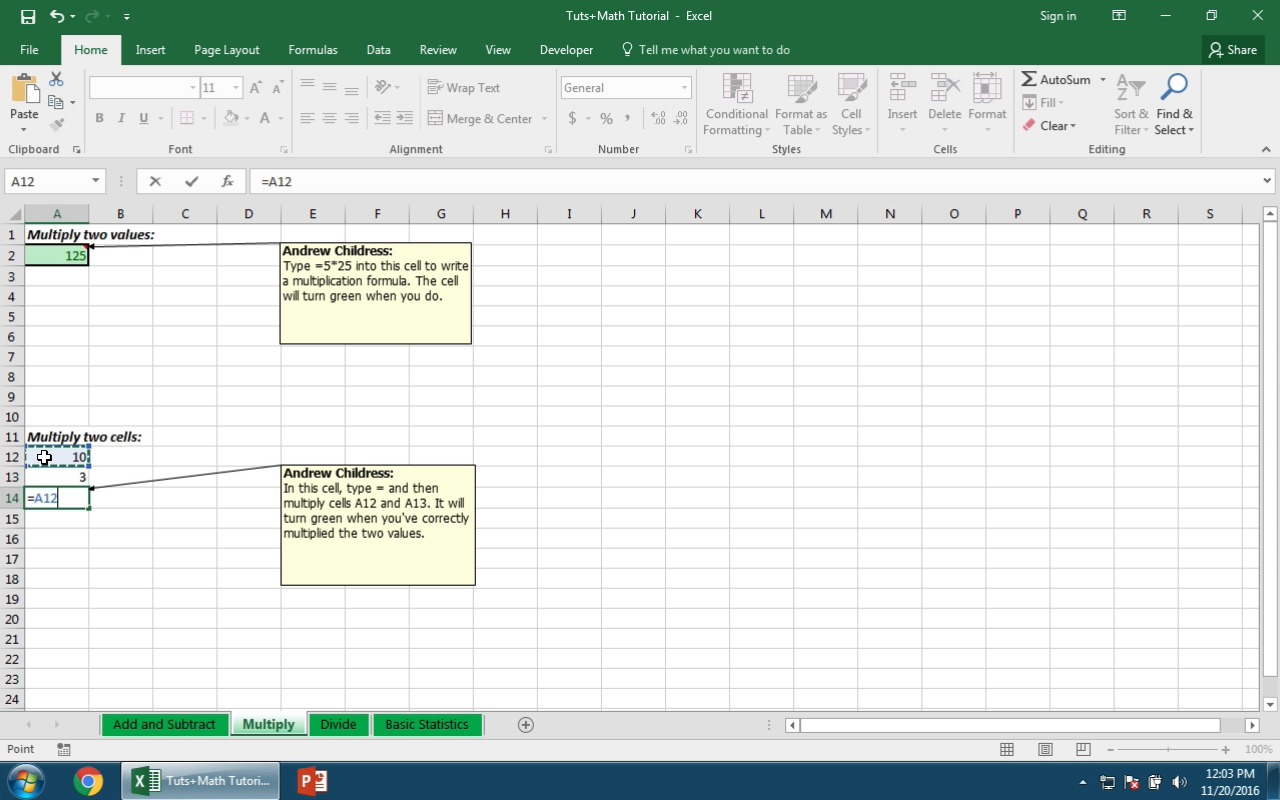
2. Multiplication
To multiply values, use the * operator. Use multiplication instead of adding the same item over and over.
Use the tab titled «Multiply» in the workbook for practice.
Example:
=5*4
or, reference values in cells with:
=A2*A3

3. Division
Division is helpful when splitting items into groups, for example. Use the «/» operator to divide numbers or the values in cells in your spreadsheet.
Use the tab titled «Divide» in the workbook for practice.
Example:
=20/10
or, reference values in cells with:
=A5/B2

Basic Statistics
Use the tab titled «Basic Statistics» in the workbook for practice.
Now that you know the basic math operators, let’s move onto something more advanced. Basic statistics are helpful to review a set of data and to make informed judgments about it. Let’s cover several popular, simple statistic formulas.
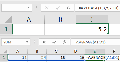
1. Average
To use an average formula in Excel, open your formula with =AVERAGE( and then input your values. Separate each number with a comma. When you press enter, Excel will calculate and output the average.
=AVERAGE(1,3,5,7,10)
The best way to calculate an average is to input your values into separate cells in a single column.
=AVERAGE(A2:A5)

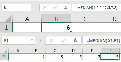
2. Median
The median of a data set is the value that’s in the middle. If you took the numerical values and ordered them from smallest to largest, the median would be smack dab in the middle of that list.
=MEDIAN(1,3,5,7,10)
I’d recommend typing your values into a list of cells, and then using the median formula over a list of cells with values typed in them.
=MEDIAN(A2:A5)

3. Min
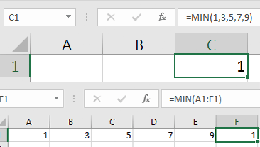
If you have a set of data and want to keep your eye on the smallest value, the MIN formula in Excel is useful. You can use the MIN formula with a list of numbers, separated by commas, to find the lowest value in a set. This is very useful when working with large datasets.
=MIN(1,3,5,7,9)
You might want to find the minimum value in a list of data, which is totally possible with a formula such as:
=MIN(A1:E1)

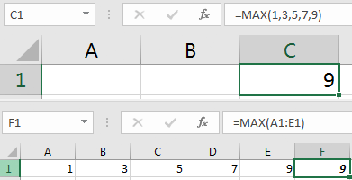
4. Max
The MAX formula in Excel is the polar opposite of MIN; it tells you which value in a set is the largest. You can use it with a list of numbers, separated by commas:
=MAX(1,3,5,7,9)
Or, you can select a list of values in cells, and have Excel return the largest in the set, with a formula like this:
=MAX(A1:E1)

Recap and Keep Learning
I hope this Excel math formulas tutorial helped you think more about what Excel can do for you. With enough practice, your Excel skills will soon seem more natural than grabbing a calculator or doing math on paper. Spreadsheets capture data, and formulas help us understand or modify that data. The operations can be basic, but are at the foundation of important spreadsheets in every company.
It’s always a great idea to use one tutorial to launch more learning. Here are some suggestions
- For more advanced math in equation-like formats, Microsoft’s official documentation has a page titled «Insert or edit an equation or expression.»
- Tuts+ instructor Bob Flisser has a nice tutorial on calculating percentages in Excel.
What are some other math skills that you use in Excel? Leave a reply in the comments if you know a great formula that I don’t.
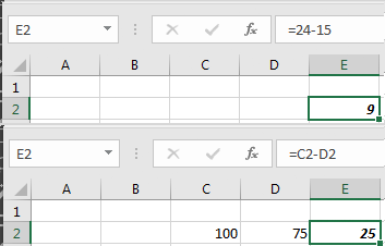
In this tutorial, I’ll show you how to perform basic math functions in Microsoft Excel. Specifically, I will show you how to add, subtract, divide and multiply cells in Excel.
So, let’s get to it.
Method 1: Use the + operation
The most basic way of adding cells is to simply do this manually by using the + operation.
=Number1+Number2
You simply replace Number1 and Number2 with the numbers your interested in, or cells containing your data.
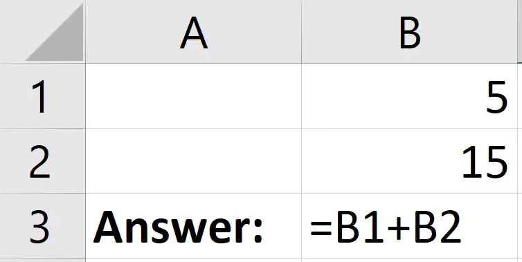
In my example, I have two cells containing the numbers 5 and 15, which I want to add together.
To do this in a new cell, I can enter the following formula.
=B1+B2
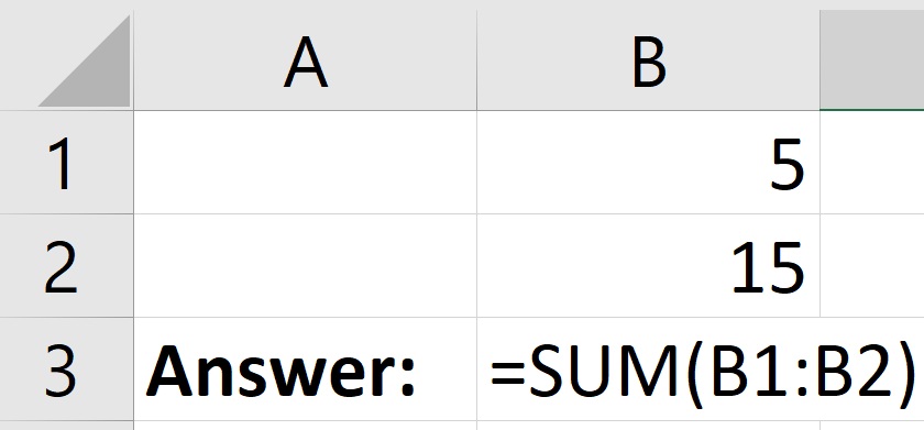
Method 2: Use the SUM function
A great thing about Excel is that it includes a function that can add a range of cells quickly for you.
To do this, use the SUM function.
=SUM(Number1, [number2],...)
Within the parentheses, simply insert the range of cells you’re interested in.
If I use the same example as shown above, I will use the following function.
=SUM(B1:B2)
How to subtract cells in Excel
To subtract numbers or cells in Excel, then use the – operation.
=Number1-Number2
Replace Number1 and Number2 with the numbers your interested in, or cells containing your data.
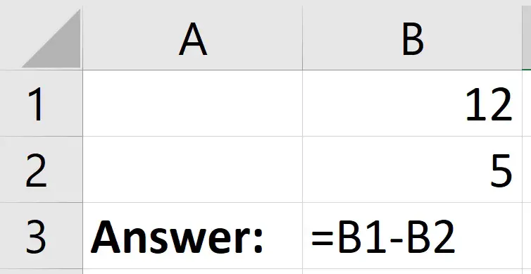
In my example below, I have two cells containing the numbers 12 and 5. I want to subtract 5 from 12.
To do this, in a new cell, I will enter the following.
=B1-B2
How to multiply cells in Excel
Method 1: Use the * operation
If you want to multiply certain numbers or specific cells together, then the easiest way to do this is by using the * operation.
=Number1*Number2
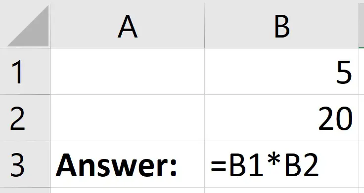
In this example, I have two cells (B1 and B2) that contain the numbers 5 and 20, repectively.
If I want to multiply these cells, I will use the following formula.
=B1*B2
Method 2: Use the PRODUCT function
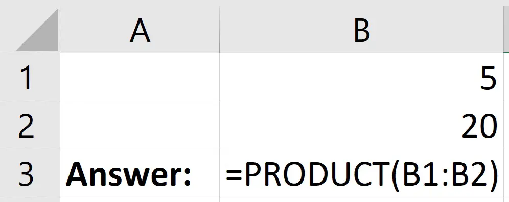
If you have a range of numbers or cells that you want to multiply together, then you can use the PRODUCT function.
=PRODUCT(Number1, [number2],...)
Within the parentheses, simply insert the range of cells you’re interested in.
For my example, the formula will look like this.
=PRODUCT(B1:B2)
How to divide cells in Excel
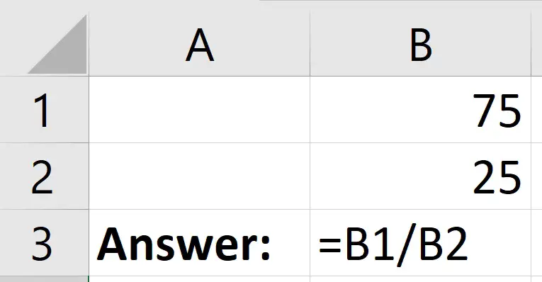
Finally, if you want to divide cells in Excel, then use the / operation.
=Number1/number2
Replace number1 and number2 with the cells you’re interested in.
For my example below, I have cells containing the values 75 (B1) and 25 (B2). If I wanted to divide 75 by 25, I will enter the following formula.
=B1/B2
How to do basic math in Excel: Final words
You should now have a better understanding of performing basic math (add, subtract, multiply and divide) in Microsoft Excel.
The table below summarises the operations you will need to perform each task.
| Calculation | Operation |
|---|---|
| Add | + |
| Subtract | – |
| Multiply | * |
| Divide | / |
If you want to add a lot of cells, then use the SUM function.
Additionally, if you want to multiply a range of cells, then use the PRODUCT function.
Microsoft Excel version used: 365 ProPlus
Содержание
- Применение математических функций
- СУММ
- СУММЕСЛИ
- ОКРУГЛ
- ПРОИЗВЕД
- ABS
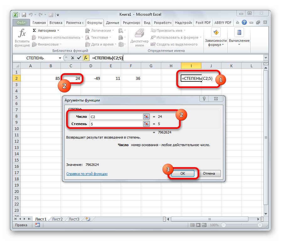
- СТЕПЕНЬ
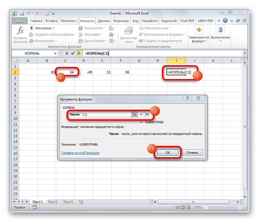
- КОРЕНЬ
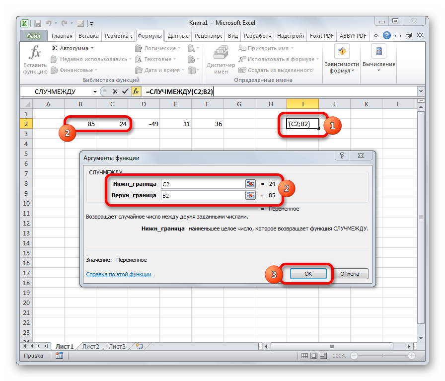
- СЛУЧМЕЖДУ
- ЧАСТНОЕ
- РИМСКОЕ
- Вопросы и ответы
Чаще всего среди доступных групп функций пользователи Экселя обращаются к математическим. С помощью них можно производить различные арифметические и алгебраические действия. Их часто используют при планировании и научных вычислениях. Узнаем, что представляет собой данная группа операторов в целом, и более подробно остановимся на самых популярных из них.
Применение математических функций
С помощью математических функций можно проводить различные расчеты. Они будут полезны студентам и школьникам, инженерам, ученым, бухгалтерам, планировщикам. В эту группу входят около 80 операторов. Мы же подробно остановимся на десяти самых популярных из них.
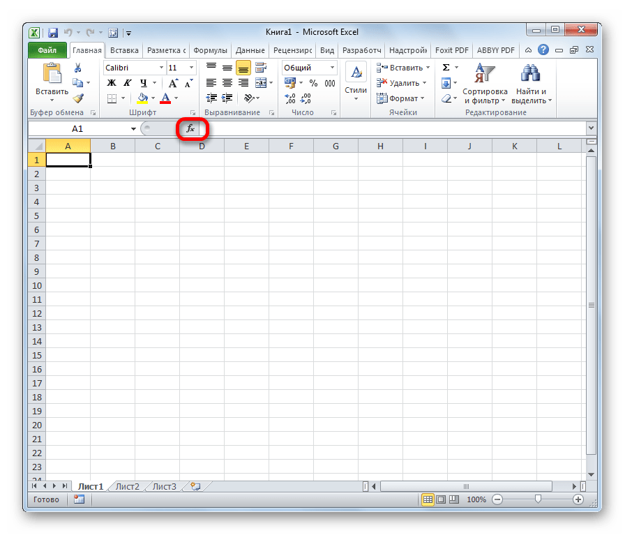
Открыть список математических формул можно несколькими путями. Проще всего запустить Мастер функций, нажав на кнопку «Вставить функцию», которая размещена слева от строки формул. При этом нужно предварительно выделить ячейку, куда будет выводиться результат обработки данных. Этот метод хорош тем, что его можно реализовать, находясь в любой вкладке.
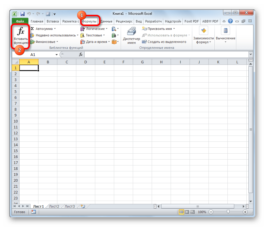
Также можно запустить Мастер функций, перейдя во вкладку «Формулы». Там нужно нажать на кнопку «Вставить функцию», расположенную на самом левом краю ленты в блоке инструментов «Библиотека функций».
Существует и третий способ активации Мастера функций. Он осуществляется с помощью нажатия комбинации клавиш на клавиатуре Shift+F3.
После того, как пользователь произвел любое из вышеуказанных действий, открывается Мастер функций. Кликаем по окну в поле «Категория».
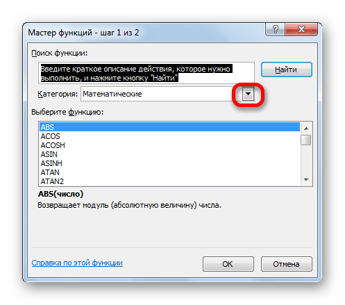
Открывается выпадающий список. Выбираем в нем позицию «Математические».
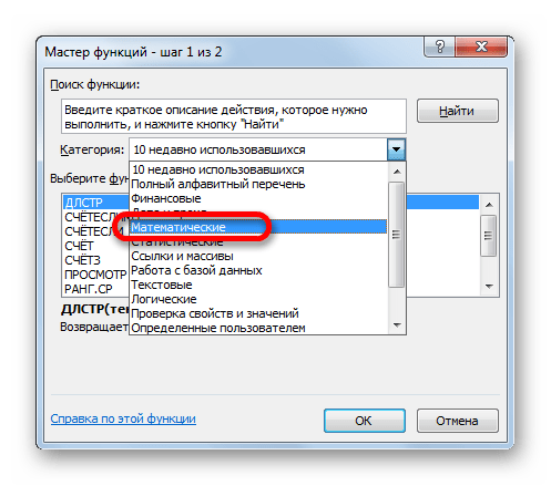
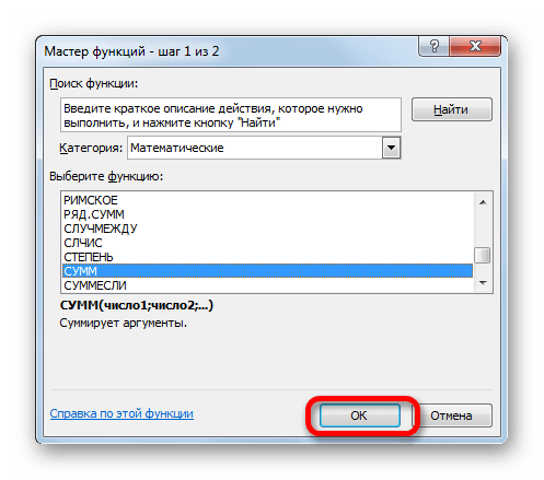
После этого в окне появляется список всех математических функций в Excel. Чтобы перейти к введению аргументов, выделяем конкретную из них и жмем на кнопку «OK».
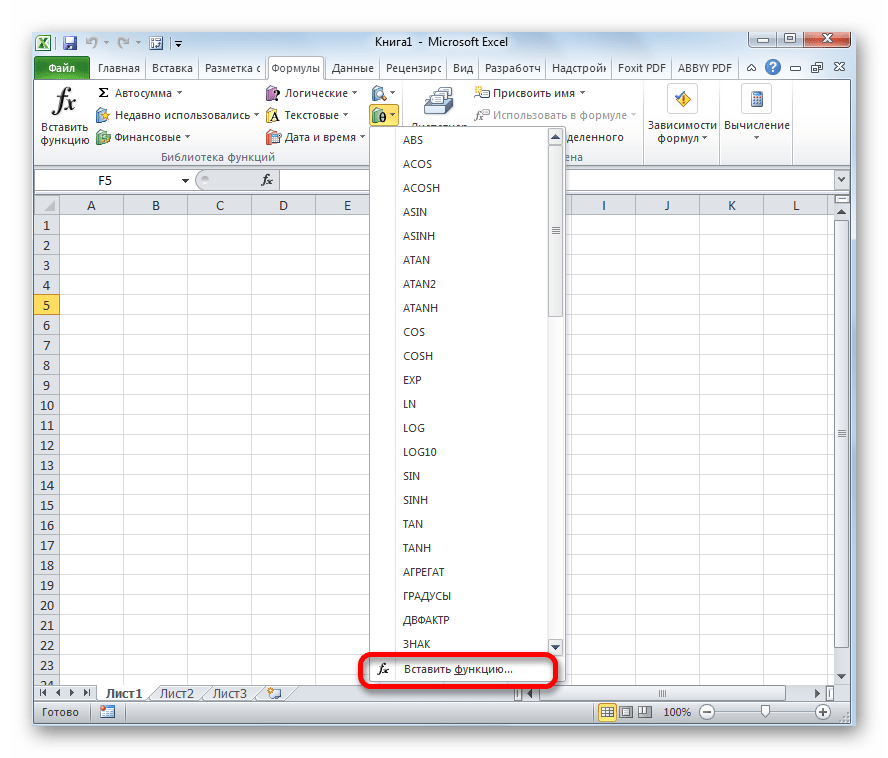
Существует также способ выбора конкретного математического оператора без открытия главного окна Мастера функций. Для этого переходим в уже знакомую для нас вкладку «Формулы» и жмем на кнопку «Математические», расположенную на ленте в группе инструментов «Библиотека функций». Открывается список, из которого нужно выбрать требуемую формулу для решения конкретной задачи, после чего откроется окно её аргументов.

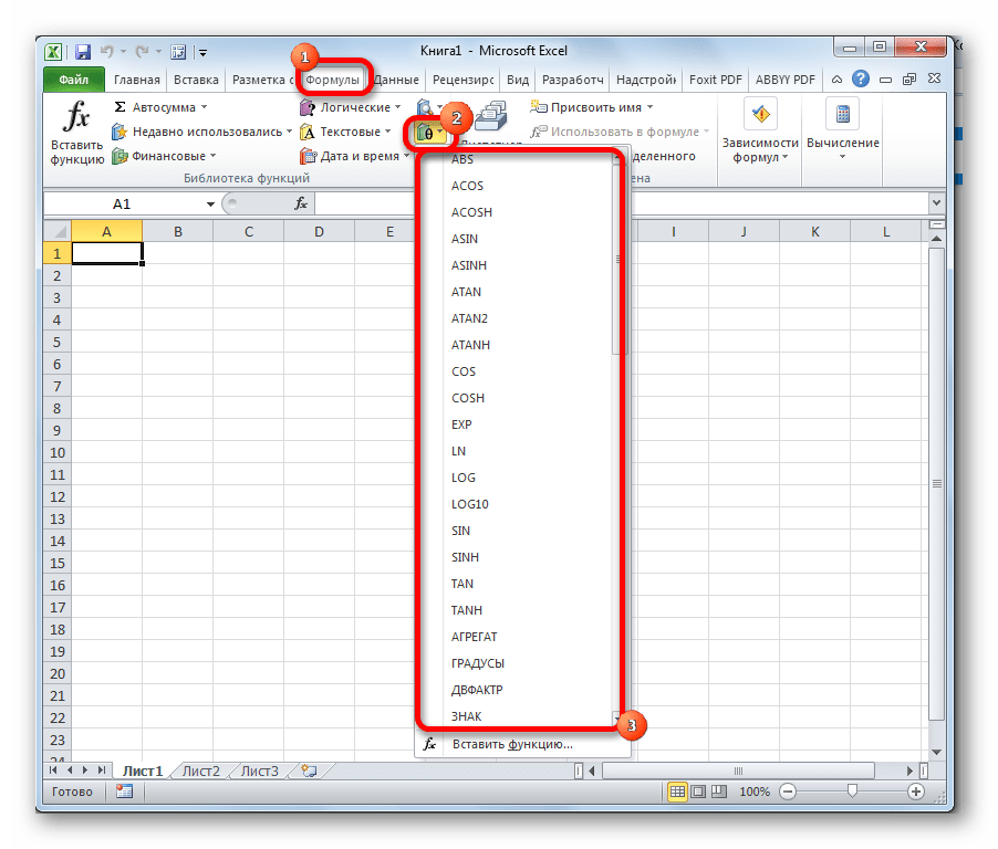
Правда, нужно заметить, что в этом списке представлены не все формулы математической группы, хотя и большинство из них. Если вы не найдете нужного оператора, то следует кликнуть по пункту «Вставить функцию…» в самом низу списка, после чего откроется уже знакомый нам Мастер функций.
Урок: Мастер функций в Excel
СУММ
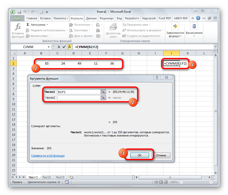
Наиболее часто используется функция СУММ. Этот оператор предназначен для сложения данных в нескольких ячейках. Хотя его можно использовать и для обычного суммирования чисел. Синтаксис, который можно применять при ручном вводе, выглядит следующим образом:
=СУММ(число1;число2;…)
В окне аргументов в поля следует вводить ссылки на ячейки с данными или на диапазоны. Оператор складывает содержимое и выводит общую сумму в отдельную ячейку.
Урок: Как посчитать сумму в Экселе
СУММЕСЛИ
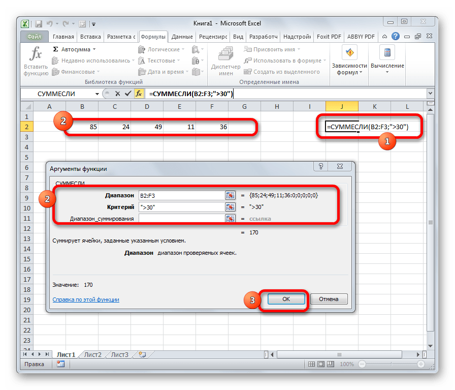
Оператор СУММЕСЛИ также подсчитывает общую сумму чисел в ячейках. Но, в отличие от предыдущей функции, в данном операторе можно задать условие, которое будет определять, какие именно значения участвуют в расчете, а какие нет. При указании условия можно использовать знаки «>» («больше»), «<» («меньше»), «< >» («не равно»). То есть, число, которое не соответствует заданному условию, во втором аргументе при подсчете суммы в расчет не берется. Кроме того, существует дополнительный аргумент «Диапазон суммирования», но он не является обязательным. Данная операция имеет следующий синтаксис:
=СУММЕСЛИ(Диапазон;Критерий;Диапазон_суммирования)
ОКРУГЛ
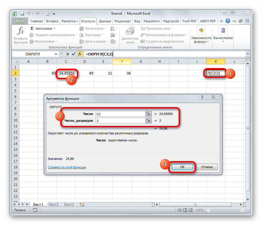
Как можно понять из названия функции ОКРУГЛ, служит она для округления чисел. Первым аргументом данного оператора является число или ссылка на ячейку, в которой содержится числовой элемент. В отличие от большинства других функций, у этой диапазон значением выступать не может. Вторым аргументом является количество десятичных знаков, до которых нужно произвести округление. Округления проводится по общематематическим правилам, то есть, к ближайшему по модулю числу. Синтаксис у этой формулы такой:
=ОКРУГЛ(число;число_разрядов)
Кроме того, в Экселе существуют такие функции, как ОКРУГЛВВЕРХ и ОКРУГЛВНИЗ, которые соответственно округляют числа до ближайшего большего и меньшего по модулю.
Урок: Округление чисел в Excel
ПРОИЗВЕД
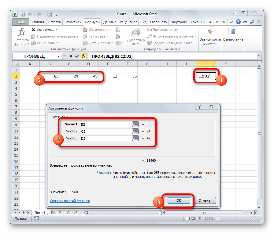
Задачей оператора ПРИЗВЕД является умножение отдельных чисел или тех, которые расположены в ячейках листа. Аргументами этой функции являются ссылки на ячейки, в которых содержатся данные для перемножения. Всего может быть использовано до 255 таких ссылок. Результат умножения выводится в отдельную ячейку. Синтаксис данного оператора выглядит так:
=ПРОИЗВЕД(число;число;…)
Урок: Как правильно умножать в Excel
ABS
С помощью математической формулы ABS производится расчет числа по модулю. У этого оператора один аргумент – «Число», то есть, ссылка на ячейку, содержащую числовые данные. Диапазон в роли аргумента выступать не может. Синтаксис имеет следующий вид:
=ABS(число)
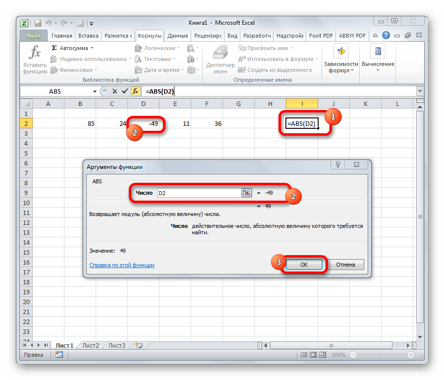
Урок: Функция модуля в Excel
СТЕПЕНЬ
Из названия понятно, что задачей оператора СТЕПЕНЬ является возведение числа в заданную степень. У данной функции два аргумента: «Число» и «Степень». Первый из них может быть указан в виде ссылки на ячейку, содержащую числовую величину. Второй аргумент указывается степень возведения. Из всего вышесказанного следует, что синтаксис этого оператора имеет следующий вид:
=СТЕПЕНЬ(число;степень)
Урок: Как возводить в степень в Экселе
КОРЕНЬ
Задачей функции КОРЕНЬ является извлечение квадратного корня. Данный оператор имеет только один аргумент – «Число». В его роли может выступать ссылка на ячейку, содержащую данные. Синтаксис принимает такую форму:
=КОРЕНЬ(число)
Урок: Как посчитать корень в Экселе
СЛУЧМЕЖДУ
Довольно специфическая задача у формулы СЛУЧМЕЖДУ. Она состоит в том, чтобы выводить в указанную ячейку любое случайное число, находящееся между двумя заданными числами. Из описания функционала данного оператора понятно, что его аргументами является верхняя и нижняя границы интервала. Синтаксис у него такой:
=СЛУЧМЕЖДУ(Нижн_граница;Верхн_граница)
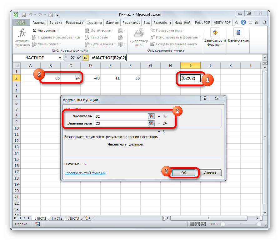
ЧАСТНОЕ
Оператор ЧАСТНОЕ применяется для деления чисел. Но в результатах деления он выводит только четное число, округленное к меньшему по модулю. Аргументами этой формулы являются ссылки на ячейки, содержащие делимое и делитель. Синтаксис следующий:
=ЧАСТНОЕ(Числитель;Знаменатель)
Урок: Формула деления в Экселе
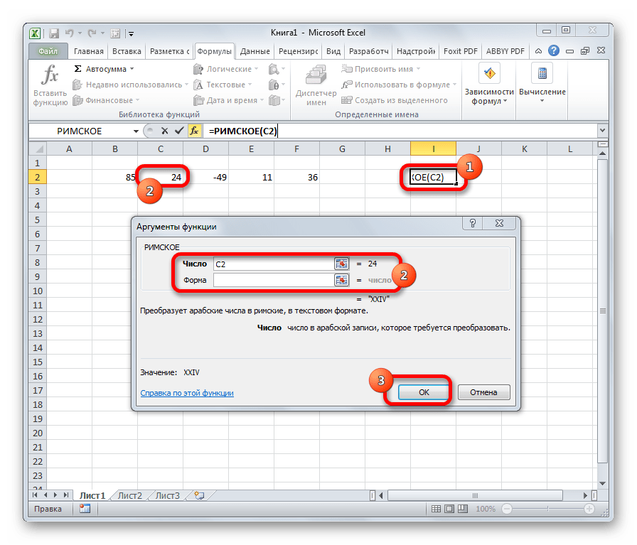
РИМСКОЕ
Данная функция позволяет преобразовать арабские числа, которыми по умолчанию оперирует Excel, в римские. У этого оператора два аргумента: ссылка на ячейку с преобразуемым числом и форма. Второй аргумент не является обязательным. Синтаксис имеет следующий вид:
=РИМСКОЕ(Число;Форма)
Выше были описаны только наиболее популярные математические функции Эксель. Они помогают в значительной мере упростить различные вычисления в данной программе. При помощи этих формул можно выполнять как простейшие арифметические действия, так и более сложные вычисления. Особенно они помогают в тех случаях, когда нужно производить массовые расчеты.
This wikiHow teaches you how to use your keyboard buttons or Excel’s pre-defined calculation formulas to make a calculation on a spreadsheet, using a desktop computer.
-

1
Open the Excel spreadsheet you want to edit. Find the spreadsheet file you want to make calculations on, and double-click on its icon to open the file.
-
2
Click on an empty cell. You can make calculations in any empty cell.
- If you make calculations in a non-empty cell, the contents of the cell will be deleted.
-
3
Type = into the empty cell. This will turn the selected cell into a formula field, and allow you to make a calculation here.
-
4
Enter the cell number of your first number. Every cell is labeled with a column letter at the top of your spreadsheet, and a row number on the left-hand side. Insert the cell number here will import the number in the indicated cell.
- For example, if you want to import a number from cell A5, type =A5.
- Alternatively, you can click the cell you want to import the number from. This will automatically add the cell number here.
- You can also just type a number here on your keyboard, like =19. You don’t have to import a number from another cell.
-
5
Type +, -, *, or / after your first cell. The sign you should be using will change depending on the type of calculation you want to make.
- Use + for addition.
- Use - for subtraction.
- Use * for multiplication.
- Use / for division.
-
6
Enter the cell number of your second number. If you’re importing your calculation numbers from another cell, type your second cell’s number here.
- If you want to use numbers from more than two cells, you can type your addition, subtraction, multiplication or division sign after your second cell, and add another cell number or value.
- For example, if you want to multiply the numbers in cells A5, A6, and B7, your formula should look like =A5*A6*B7.
-
7
Hit ↵ Enter or ⏎ Return on your keyboard. This will make your calculation, and return the result in the formula cell.


-
1
Open the Excel spreadsheet you want to edit. Find the spreadsheet file you want to make calculations on, and double-click on its icon to open the file.
-
2
Click on an empty cell. You can make calculations in any empty cell.
- If you make calculations in a non-empty cell, the contents of the cell will be deleted.
-
3
Click the fx button at the top. You can find this button below the toolbar ribbon in the upper-left corner of your spreadsheet. It will turn this cell into a formula field, and open a list of the available formulas.
-
4
Double-click the formula you want to use. You can calculate the average of several values, make summations, or calculate more complicated statistics such as standard deviation or percentile.
- This will insert the selected formula into the selected cell.
-
5
Fill out the inside of the formula. Click inside the parentheses next to your formula in the formula cell, and enter the numbers of all the cells you want to use in your calculation.
- Depending on the formula, the order of the cell numbers may change. You can click the formula on the formula list to see its breakdown.
- For example, the order doesn’t matter for the =SUM() summation formula. If you’re using a more complicated formula like =POWER(), you’ll have to enter the base number first, and then the power exponent.
- Make sure to separate each cell number in the formula with a comma.
-
6
Hit ↵ Enter or ⏎ Return on your keyboard. This will make your calculation, and return the result in the selected cell.


Ask a Question
200 characters left
Include your email address to get a message when this question is answered.
Submit
About this article
Article SummaryX
1. Open an Excel spreadsheet.
2. Click an empty cell.
3. Type «=» and enter your calculation, or click fx at the top to select a formula.
4. Hit Enter or Return on your keyboard to see the result.
Did this summary help you?
Thanks to all authors for creating a page that has been read 101 times.
Is this article up to date?
Содержание
- Основные математические формулы в Excel (смотрите и учитесь)
- Основы Формул
- 1. Каждая формула в Excel начинается с “=”
- 2. Формулы показываются на панели формул Excel.
- 3. Как собрать формулу
- Базовая статистика
- Среднее
- Медиана
- Минимум
- Максимум
- Циклические вычисления
- Циклические вычисления и нахождение корней уравнения
- Функции ЧЁТН и НЕЧЁТ
- Функции ОКРВНИЗ, ОКРВВЕРХ
- Функции ЦЕЛОЕ и ОТБР
- Функция ПРОИЗВЕД
- Функция ОСТАТ
- Функция КОРЕНЬ
- Функция ЧИСЛОКОМБ
- Функция ЕЧИСЛО
- Формула ЧАСТНОЕ()
- Формула СУММЕСЛИ()
- Формулы ОКРУГЛ(), ОКРУГЛВВЕРХ(), ОКРУГЛВНИЗ()
- Использование ссылок
- ABS
- СТЕПЕНЬ
- СЛУЧМЕЖДУ
- РИМСКОЕ
- LOG
- Заключение
Если изучение по видеороликам, это ваш стиль, посмотрите видео ниже, чтобы пройти по этому уроку. В противном случае продолжайте читать подробное описание того, как работать с каждой математической формулой Excel.
Основы Формул
Прежде чем мы начнем, давайте рассмотрим, как использовать любую формулу в Microsoft Excel. Независимо от того, работаете ли вы с математическими формулами в этом учебнике или любыми другими, эти советы помогут вам овладеть Excel.
1. Каждая формула в Excel начинается с “=”
Чтобы ввести формулу, щелкните любую ячейку в Microsoft Excel и введите знак равенства на клавиатуре. Так начинается формула.

После знака равенства вы можете размещать в ячейке невероятно разнообразные вещи. Попробуйте ввести =4+4 в качестве вашей первой формулы и нажмите Enter, чтобы отобразить результат. Excel выведет 8, но формула останется за кулисами электронной таблицы.
2. Формулы показываются на панели формул Excel.
Когда вы вводите формулу в ячейку, вы можете увидеть результат в ячейке сразу после нажатия клавиши ввода. Но когда вы выбираете ячейку, вы можете увидеть формулу для этой ячейки на панели формул.

Чтобы использовать пример выше, ячейка отобразит «8», но когда мы нажмем на эту ячейку, панель формул покажет, что ячейка складывает 4 и 4.
3. Как собрать формулу
В приведенном выше примере мы набрали простую формулу для складывания двух чисел. Но вам не обязательно вводить числа, вы также можете ссылаться на другие ячейки.
Excel — это сетка ячеек, а столбцы идут слева направо, каждая назначена на букву, а строки пронумерованы. Каждая ячейка является пересечением строки и столбца. Например, ячейка, где пересекаются столбцы A и строка 3, называется A3.

Предположим, что у меня две ячейки с простыми числами, например 1 и 2, и они находятся в ячейках A2 и A3. Когда я набираю формулу, я могу начать формулу с «=», как всегда. Затем я могу ввести:
=A2+A3
…чтобы сложить эти два числа вместе. Очень распространено иметь лист со значениями и отдельный лист, где выполняются вычисления. Соблюдайте все эти советы при работе с этим руководством. Для каждой из формул вы можете ссылаться на ячейки или непосредственно вводить числовые значения в формулу.
Если вам нужно изменить формулу, которую вы уже набрали, дважды щелкните по ячейке. Вы сможете настроить значения в формуле.
Базовая статистика
Используйте вкладку “Basic Statistics” в книге для практики.
Теперь, когда вы знаете основные математические операторы, давайте перейдем к чему-то более продвинутому. Базовая статистика полезна для обзора набора данных и принятия обоснованных решений. Давайте рассмотрим несколько популярных простых статистических формул.
Среднее
Чтобы использовать формулу среднего в Excel, начните формулу с помощью =СРЗНАЧ(, а затем введите свои значения. Разделите каждое число запятой. Когда вы нажмёте клавишу ввода, Excel вычислит и выведет среднее значение.
=СРЗНАЧ(1;3;5;7;10)
Лучший способ рассчитать среднее это ввести ваши значения в отдельные ячейки в одном столбце.
=СРЗНАЧ(A2:A5)

Медиана
Медиана набора данных это значение, которое находится посередине. Если вы взяли числовые значения и выставили их в порядке от наименьшего к самому большому, медиана была бы ровно посередине этого списка.
=МЕДИАНА(1;3;5;7;10)
Я бы рекомендовал ввести ваши значения в список ячеек, а затем использовать формулу медианы над списком ячеек со значениями, введенными в них.
=МЕДИАНА(A2:A5)

Минимум
Если у вас есть набор данных и вы хотите держать на виду наименьшее значение, полезно использовать формулу МИН в Excel. Вы можете использовать формулу МИН со списком чисел, разделенных точкой с запятыми, чтобы найти самое маленькое значение в наборе. Это очень полезно при работе с большими наборами данных.
=МИН(1;3;5;7;9)
Возможно, вы захотите найти минимальное значение в списке данных, что вполне возможно с помощью такой формулы, как:
=МИН(A1:E1)

Максимум
Формула МАКС в Excel — полная противоположность МИН
=МАКС(1;3;5;7;9)
Или же, вы можете выбрать список значений в ячейках, и Excel вернет наибольшее из набора с этой формулой:
=МАКС(A1:E1)

Циклические вычисления
Если зависимые ячейки Excel образуют цикл, то говорят, что имеют место циклические ссылки (circular references). В обычном режиме Excel обнаруживает цикл и выдает сообщение о возникшей ситуации, требуя устранить циклические ссылки. Следуя обычной семантике, он не может провести вычисления, так как циклические ссылки порождают бесконечные вычисления. Есть два выхода из этой ситуации, – устранить циклические ссылки или изменить настройку в машине вычислений так, чтобы такие вычисления стали возможными. В последнем случае, естественно, требуется, чтобы число повторений цикла было конечным. Excel допускает переход к новой семантике, обеспечивающей проведение циклических вычислений. Вручную, для этого достаточно на вкладке Вычисления (меню Сервис, пункт Параметры) включить флажок Итерации и при необходимости изменить число повторений цикла в окошке “Максимум итераций”. Можно также задать точность вычислений в окошке “Максимальное изменение”, что также приводит к ограничению числа повторений цикла. По умолчанию максимальное число итераций и точность вычислений соответственно имеют значения 100 и 0,0001. Понятно, что включить циклические вычисления и задать значения параметров, определяющих окончание цикла, можно и программно.
Укажем, особенности семантики циклических вычислений:
- Формулы, связанные циклическими ссылками, вычисляются многократно.
- Запись формул на листе определяет порядок их вычисления. Формулы вычисляются сверху вниз, слева направо.
- Число повторений цикла определяется параметрами, заданными на вкладке Вычисления. Цикл заканчивается при достижении максимального числа итераций или, когда изменения значений во всех ячейках не превосходят заданной точности.
В каких же ситуациях требуется прибегать к циклическим вычислениям? Это, возможно, следует делать, когда речь идет о реализации итерационного процесса, вычислениях по рекуррентным соотношениям. У нас уже были примеры реализации итерационных процессов, например, вычисление суммы ряда, задающего экспоненту, в которых не применялись циклические ссылки. Платой за это было использование дополнительных ячеек таблицы Excel. Правда, появлялись и новые возможности, – возможность построить график, проанализировать процесс сходимости и т.д. Тем не менее, программисту, привыкшему к традиционным языкам, и привыкшему “с детства” экономить на переменных, может показаться странным предложенное решение задачи о нахождении корня уравнения, где на экран выводятся результаты всех приближений. В Excel экономия ячеек не главная задача. Тем не менее, при реализации итерационных процессов можно, конечно, и в Excel иметь одну единственную ячейку X, значение которой изменяется, начиная от начального приближения до искомого результата. Это в большей степени соответствует понятию переменной в языках программирования.
Циклические вычисления и нахождение корней уравнения
Покажем, как можно использовать циклические вычисления на примере задачи нахождения корня уравнения методом Ньютона. Для простоты я начну с квадратного уравнения, а позже рассмотрю и более “серьезные” уравнения. Итак, рассмотрим квадратное уравнение: X2 -5X+6 =0. Найти корень этого (и любого другого уравнения) можно, используя всего одну единственную ячейку Excel. Для этого достаточно включить режим циклических вычислений и ввести в произвольную ячейку с именем, скажем X, рекуррентную формулу, задающую вычисления по Ньютону:
где F и F1 задают соответственно выражения, вычисляющие функцию и производную. Для нашего квадратного уравнения после ввода формулы в ней появится значение 2, соответствующее одному из корней уравнения. А как получить второй корень? Обычно, это можно сделать путем изменения начального приближения. В нашем случае начальное приближение не задавалось, итерационный процесс вычислений начинался со значения, хранимого в ячейке X по умолчанию и равного нулю. Как же задать начальное приближение в циклических вычислениях? Возникшая проблема не связана с данной конкретной задачей. Она возникает всегда в циклических вычислениях, – до начала цикла надо задать начальные установки. В рекуррентных соотношениях всегда есть некоторый начальный отрезок. Решать задачу задания начальных установок в каждом случае можно по-разному. Я продемонстрирую один прием, основанный на использовании функции ЕСЛИ. Вот как выглядит “настоящее” решение этой задачи, использующее 4 ячейки, две из которых нужны по существу дела, а две используются для повышения наглядности процесса вычислений:
- В ячейку с именем Xinit я ввел начальное приближение.
- В ячейку Xcur, в которой и будет идти циклический счет, ввел формулу:
= ЕСЛИ(Xcur =0; Xinit; Xcur - (6- Xcur *(5- Xcur))/(2* Xcur -5))
- В две другие вспомогательные ячейки я поместил текст этой формулы и формулу, задающую вычисление функции в точке Xcur, позволяющую следить за качеством решения.
- Заметьте, что на первом шаге вычислений, функция IF (ЕСЛИ) поместит в ячейку Xcur начальное значение, а затем уже начнет счет по формуле на последующих шагах.
- Чтобы сменить начальное приближение, недостаточно изменить содержимое ячейки Xinit и запустить процесс вычислений. В этом случае вычисления будут продолжены, начиная с последнего вычисленного значения. Чтобы обнулить значение, хранящееся в ячейке Xcur, нужно заново записать туда формулу. Для этого достаточно выбрать ячейку и выделить текст формулы непосредственно в окне ее редактирования. Щелчок по Enter начнет вычисления с новым начальным приближением.
Функции ЧЁТН и НЕЧЁТ
Для выполнения операций округления можно использовать функции ЧЁТН (EVEN) и НЕЧЁТ (ODD). Функция ЧЁТН округляет число вверх до ближайшего четного целого числа. Функция НЕЧЁТ округляет число вверх до ближайшего нечетного целого числа. Отрицательные числа округляются не вверх, а вниз. Функции имеют следующий синтаксис:
=ЧЁТН(число)
=НЕЧЁТ(число)
Функции ОКРВНИЗ, ОКРВВЕРХ
Функции ОКРВНИЗ (FLOOR) и ОКРВВЕРХ (CEILING) тоже можно использовать для выполнения операций округления. Функция ОКРВНИЗ округляет число вниз до ближайшего кратного для заданного множителя, а функция ОКРВВЕРХ округляет число вверх до ближайшего кратного для заданного множителя. Эти функции имеют следующий синтаксис:
=ОКРВНИЗ(число;множитель)
=ОКРВВЕРХ(число;множитель)
Значения число и множитель должны быть числовыми и иметь один и тот же знак. Если они имеют различные знаки, то будет выдана ошибка.
Функции ЦЕЛОЕ и ОТБР
Функция ЦЕЛОЕ (INT) округляет число вниз до ближайшего целого и имеет следующий синтаксис:
=ЦЕЛОЕ(число)
Аргумент – число – это число, для которого надо найти следующее наименьшее целое число.
Рассмотрим формулу:
=ЦЕЛОЕ(10,0001)
Эта формула возвратит значение 10, как и следующая:
=ЦЕЛОЕ(10,999)
Функция ОТБР (TRUNC) отбрасывает все цифры справа от десятичной запятой независимо от знака числа. Необязательный аргумент количество_цифр задает позицию, после которой производится усечение. Функция имеет следующий синтаксис:
=ОТБР(число;количество_цифр)
Если второй аргумент опущен, он принимается равным нулю. Следующая формула возвращает значение 25:
=ОТБР(25,490)
Функции ОКРУГЛ, ЦЕЛОЕ и ОТБР удаляют ненужные десятичные знаки, но работают они различно. Функция ОКРУГЛ округляет вверх или вниз до заданного числа десятичных знаков. Функция ЦЕЛОЕ округляет вниз до ближайшего целого числа, а функция ОТБР отбрасывает десятичные разряды без округления. Основное различие между функциями ЦЕЛОЕ и ОТБР проявляется в обращении с отрицательными значениями. Если вы используете значение -10,900009 в функции ЦЕЛОЕ, результат оказывается равен -11, но при использовании этого же значения в функции ОТБР результат будет равен -10.
Функция ПРОИЗВЕД
Функция ПРОИЗВЕД (PRODUCT) перемножает все числа, задаваемые ее аргументами, и имеет следующий синтаксис:
=ПРОИЗВЕД(число1;число2…)
Эта функция может иметь до 30 аргументов. Excel игнорирует любые пустые ячейки, текстовые и логические значения.
Функция ОСТАТ
Функция ОСТАТ (MOD) возвращает остаток от деления и имеет следующий синтаксис:
=ОСТАТ(число;делитель)
Значение функции ОСТАТ – это остаток, получаемый при делении аргумента число на делитель. Например, следующая функция возвратит значение 1, то есть остаток, получаемый при делении 19 на 14:
=ОСТАТ(19;14)
Если число меньше чем делитель, то значение функции равно аргументу число. Например, следующая функция возвратит число 25:
=ОСТАТ(25;40)
Если число точно делится на делитель, функция возвращает 0. Если делитель равен 0, функция ОСТАТ возвращает ошибочное значение.
Функция КОРЕНЬ
Функция КОРЕНЬ (SQRT) возвращает положительный квадратный корень из числа и имеет следующий синтаксис:
=КОРЕНЬ(число)
Аргумент число должен быть положительным числом. Например, следующая функция возвращает значение 4:
КОРЕНЬ(16)
Если число отрицательное, КОРЕНЬ возвращает ошибочное значение.
Функция ЧИСЛОКОМБ
Функция ЧИСЛОКОМБ (COMBIN) определяет количество возможных комбинаций или групп для заданного числа элементов. Эта функция имеет следующий синтаксис:
=ЧИСЛОКОМБ(число;число_выбранных)
Аргумент число – это общее количество элементов, а число_выбранных – это количество элементов в каждой комбинации. Например, для определения количества команд с 5 игроками, которые могут быть образованы из 10 игроков, используется формула:
=ЧИСЛОКОМБ(10;5)
Результат будет равен 252. Т.е., может быть образовано 252 команды.
Функция ЕЧИСЛО
Функция ЕЧИСЛО (ISNUMBER) определяет, является ли значение числом, и имеет следующий синтаксис:
=ЕЧИСЛО(значение)
Пусть вы хотите узнать, является ли значение в ячейке А1 числом. Следующая формула возвращает значение ИСТИНА, если ячейка А1 содержит число или формулу, возвращающую число; в противном случае она возвращает ЛОЖЬ:
=ЕЧИСЛО(А1)
Формула ЧАСТНОЕ()
Тоже одна из простых операций в математике. В Экселе выполняется тоже несложно: у функции ЧАСТНОЕ() есть два аргумента: делимое и делитель.
В выделенной ячейке выводится частное:

Формула СУММЕСЛИ()
Оператор СУММЕСЛИ() находит сумму чисел. Главное отличие этой функции от СУММ() в том, что здесь в качестве аргумента можно задавать условие (только одно), которое будет показывать, какие значения будут использованы в расчетах, а какие — нет.
В качестве условий могут выступать неравенства со знаками больше, меньше или не равно («>», «<», «< >»). Число, которое не соответствует введенному условию, не будет включен в суммирование.
На рисунке изображено суммирование всех чисел, которые больше 0.
Оранжевым выделены те числа, которые будут включены в расчет функцией СУММЕСЛИ().
Остальные числа просто будут игнорироваться:

Например, нужно посчитать общую стоимость всех проданных фруктов.
Для этого воспользуемся следующей формулой:

Формулы ОКРУГЛ(), ОКРУГЛВВЕРХ(), ОКРУГЛВНИЗ()
Функция ОКРУГЛ() предназначена для округления значения до заданного количества знаков после запятой. В качестве первого аргумента выступают, как обычно, числа или диапазон ячеек, второго – разряд, до которого нужно округлить число.
Например, округление значения до второго знака после запятой:

Если в качестве второго аргумента выступает 0, то число будет округляться до ближайшего целого:

Второй аргумент может быть и отрицательным, тогда округление будет происходить до требуемого знака перед запятой:

Если необходимо округлить в сторону меньшего или большего по модулю числа используют функции ОКРУГЛВНИЗ(), ОКРУГЛВВЕРХ(), соответственно:


Замечание: многие могут решить, что функции округления бесполезны, так как можно просто убрать/добавить дополнительный знак после запятой с помощью кнопок увеличить/уменьшить разрядность.
На самом деле, это не так.
Дело в том, что увеличение или уменьшение разрядности влияет только на «внешний вид» ячейки, то есть на то, как мы число видим.
Само число, при этом, не меняется. Функции округления же полностью меняют вид числа, убирая лишние разряды.
Использование ссылок
При работе с Excel можно применять в работе различные виды ссылок. Начинающим пользователям доступны простейшие из них. Важно научиться использовать все форматы в своей работе.
Существуют:
- простые;
- ссылки на другой лист;
- абсолютные;
- относительные ссылки.
Простые адреса используются чаще всего. Простые ссылки могут быть выражены следующим образом:
- пересечение столбца и строки (А4);
- массив ячеек по столбцу А со строки 5 до 20 (А5:А20);
- диапазон клеток по строке 5 со столбца В до R (В5:R5);
- все ячейки строки (10:10);
- все клетки в диапазоне с 10 по 15 строку (10:15);
- по аналогии обозначаются и столбцы: В:В, В:К;
- все ячейки диапазона с А5 до С4 (А5:С4).
Следующий формат адресов: ссылки на другой лист. Оформляется это следующим образом: Лист2!А4:С6. Подобный адрес вставляется в любую функцию.
ABS
С помощью математической формулы ABS производится расчет числа по модулю. У этого оператора один аргумент – «Число», то есть, ссылка на ячейку, содержащую числовые данные. Диапазон в роли аргумента выступать не может. Синтаксис имеет следующий вид:
=ABS(число)

СТЕПЕНЬ
Из названия понятно, что задачей оператора СТЕПЕНЬ является возведение числа в заданную степень. У данной функции два аргумента: «Число» и «Степень». Первый из них может быть указан в виде ссылки на ячейку, содержащую числовую величину. Второй аргумент указывается степень возведения. Из всего вышесказанного следует, что синтаксис этого оператора имеет следующий вид:
=СТЕПЕНЬ(число;степень)

СЛУЧМЕЖДУ
Довольно специфическая задача у формулы СЛУЧМЕЖДУ. Она состоит в том, чтобы выводить в указанную ячейку любое случайное число, находящееся между двумя заданными числами. Из описания функционала данного оператора понятно, что его аргументами является верхняя и нижняя границы интервала. Синтаксис у него такой:
=СЛУЧМЕЖДУ(Нижн_граница;Верхн_граница)

РИМСКОЕ
Данная функция позволяет преобразовать арабские числа, которыми по умолчанию оперирует Excel, в римские. У этого оператора два аргумента: ссылка на ячейку с преобразуемым числом и форма. Второй аргумент не является обязательным. Синтаксис имеет следующий вид:
=РИМСКОЕ(Число;Форма)

LOG
С помощью этого оператора определяется логарифм числа по заданному основанию. Синтаксис функции представлен в виде:
=LOG(Число;Основание)
Необходимо заполнить два аргумента: Число и Основание логарифма (если его не указать, программа примет значение по умолчанию, равное 10).

Также для десятичного логарифма предусмотрена отдельная функция – LOG10.
Заключение
Таким образом, мы разобрали самые популярные математические функции, которые используются в Excel. Однако возможности программы гораздо шире, и в ее инструментарии можно найти функцию для успешного выполнения практически любой задачи.
Источники
- https://business.tutsplus.com/ru/tutorials/how-to-use-excel-math-formulas–cms-27554
- https://www.intuit.ru/studies/courses/114/114/lecture/3315
- http://on-line-teaching.com/excel/lsn021.html
- https://blog.sf.education/matematicheskie-funkczii-v-excel/
- https://FB.ru/article/445487/matematicheskie-funktsii-v-excel-osobennosti-i-primeryi
- https://lumpics.ru/mathematical-functions-in-excel/
- https://MicroExcel.ru/matematicheskie-funktsii/
How do I calculate in Excel on my computer?
How to do calculations in Excel
- Type the equal symbol (=) in a cell. This tells Excel that you are entering a formula, not just numbers.
- Type the equation you want to calculate. For example, to add up 5 and 7, you type =5+7.
- Press the Enter key to complete your calculation. Done!
How do I insert a math function in Excel?
How do you add up cells in Excel on a Mac?
The easiest way to add a SUM formula to your worksheet is to use AutoSum. Select an empty cell directly above or below the range that you want to sum, and on the Home or Formula tabs of the ribbon, click AutoSum > Sum.
Where is the use in formula button in Excel on a Mac?
How?
- Click the first empty cell below a column of numbers.
- Do one of the following: Excel 2016 for Mac: : On the Home tab, click AutoSum. Excel for Mac 2011: On the Standard toolbar, click AutoSum.
- Press RETURN .
How can I be brilliant in maths?
To show the Formula Bar, click the View tab, and then click to select the Formula Bar check box. Tip: If you want to expand the Formula Bar to show more of the formula, press CONTROL+SHIFT+U.
How do I create a custom formula in Excel?
Just select all the cells at the same time, then enter the formula normally as you would for the first cell. Then, when you’re done, instead of pressing Enter, press Control + Enter. Excel will add the same formula to all cells in the selection, adjusting references as needed.
Why is math so hard?
How can I get full marks in maths?
Follow along to create custom functions:
- Press Alt + F11.
- Choose Insert→Module in the editor.
- Type this programming code, shown in the following figure:
- Save the function.
- Return to Excel.
- Click the Insert Function button on the Formulas tab to display the Insert Function dialog box.
- Click OK.
How can I be a genius in maths?
Why do we learn useless math?
Math seems difficult because it takes time and energy. Many people don’t experience sufficient time to “get” math lessons, and they fall behind as the teacher moves on. Many move on to study more complex concepts with a shaky foundation. We often end up with a weak structure that is doomed to collapse at some point.
Why is math so stressful?
Here’s how I studied.
- Self-study NCERT completely.
- Solve all the exercises.
- Solve all the examples.
- If not understood well, repeat this.
- Come up with questions and take guidance from your teachers.
- Solve sample question papers.
- Last 20 days of practice – most crucial.
How do you help students struggle with math?
Is math harder than science?
Learn the Logic and Process Involved in Solving a Problem
Instead, try to understand the concepts behind math. If you see how and why an equation works, you’ll be able to remember it more easily in a pinch. Math theory may seem complicated, but with a little hard work you can begin to figure it out.
What is the most useless subject?
Math is not entirely useless. It teaches you basics that can help you later in life. So when you learn “useless math”, you are actually learning basic skills of problem solving that you will most definitely need at least once in your life time. School is not to entertain you, but to prepare you for life.
Is math really necessary?
What is the easiest subject?
What Causes Math Anxiety? The deadlines that timed tests impose on students lead them to feel anxious. This leads them to forget concepts that they have no problem remembering at home. Since these tests can have a negative impact on grades, the student’s fear of failure is confirmed.
What is the hardest subject in the world?
What is the hardest subject in math?
Check out these top 5 math strategies you can use.
- Math Strategies: Master the Basics First. Image by RukiMedia.
- Help Them Understand the Why. Struggling students need plenty of instruction.
- Make It a Positive Experience. Image by stockfour.
- Use Models and Learning Aids.
- Encourage Thinking Out Loud.
What is the easiest thing to study?
On average, pure math is about the same level of difficulty as physics, Probably harder for the average individual than chemistry, etc. There are many different sciences and types of math. Even then some people are gifted in science, some in math, some in music, reading, or writing. It’s all relative.
7 Mathematical Functions used in MS Excel with Examples
- SUM
- AVERAGE
- AVERAGEIF
- COUNTA
- COUNTIF
- MOD
- ROUND
Table of contents
- 7 Mathematical Functions used in MS Excel with Examples
- #1 SUM
- #2 AVERAGE
- #3 AVERAGEIF
- #4 COUNTA
- #5 COUNTIF
- #6 MOD
- #7 ROUND
- Things to Remember
- Recommended Articles

You are free to use this image on your website, templates, etc, Please provide us with an attribution linkArticle Link to be Hyperlinked
For eg:
Source: Mathematical Function in Excel (wallstreetmojo.com)
Let us discuss each of them in detail.
You can download this Mathematical Function Excel Template here – Mathematical Function Excel Template
#1 SUM
If we want to SUM values of several cells quickly, we can use the SUM in excelThe SUM function in excel adds the numerical values in a range of cells. Being categorized under the Math and Trigonometry function, it is entered by typing “=SUM” followed by the values to be summed. The values supplied to the function can be numbers, cell references or ranges.read more for the mathematics category.
For example, look at the below data in Excel.

We need to find the total production quantity and total salary from this.

Open the SUM function in the G2 cell.

And select the range of cells from C2 to C11.

Close the bracket and press the “Enter” key to get the total production quantity.

So, the total production quantity is 1,506. Similarly, we must apply the same logic to get the total salary amount.

#2 AVERAGE
Now, we know what overall sum values are. Next, we need to find the average salary per employee out of these overall employees.

Open the AVERAGE functionThe AVERAGE function in Excel gives the arithmetic mean of the supplied set of numeric values. This formula is categorized as a Statistical Function. The average formula is =AVERAGE(read more in the G4 cell.

Select the range of cells for which we are finding the average value, so our range of cells will be from D2 to D11.

So the average salary per person is $4,910.
#3 AVERAGEIF
We know the average salary per person; we want to know the average salary based on gender for further drill-down. What is the average salary of males and females?
- We can achieve this by using the AVERAGEIF function.

- The first parameter of this function is range. For example, choose cells from B2 to B11.

- We need to consider only male employees in this range, so enter the criteria as “M.”

- Next, we need to choose the average range, D1 to D11.

- So, the average salary of male employees is $4,940. Similarly, we must apply the formula to find the average female salary.

The female average salary is $4,880.
#4 COUNTA
Let us find out how many employees are there in this range.
- To find the number of employees, we need to use the COUNTA function in excel.

The COUNTA function will count the number of non-empty cells in the selected range of cells. So totally, there are 10 employees on the list.
#5 COUNTIF
After counting the total number of employees, we may need to count how many male and female employees there are.
- So we can do this by using the “COUNTIF” function. The COUNTIF counts the cells based on the criteria given.

- The range is in which range of cells we need to count since we need to count the number of male or female employees who choose cells from B2 to B11.

- The criteria will be in the selected range. What do we need to count? Since we need to count how many male employees there are, give the criteria as “M.”

- Similarly, copy the formula and change the criteria from “M” to “F.”

#6 MOD
The MOD function will return the remainder when one number is divided by another. For example, dividing the number 11 by 2 will get the remainder as 1 because only till 10 number 2 can divide.
- For example, look at the below data.

- By applying a simple MOD function, we can find the remainder value.

#7 ROUND
When we have fraction or decimal values, we may need to round those decimal values to the nearest integer number. For example, we need to round the numbers 3.25 to 3 and 3.75 to 4.
- We can do this by using a ROUND function in excel.

- Open ROUND functionROUND is a built-in Excel function that calculates the round number of a given number using the number of digits as an argument. The number to be rounded up to and the number of digits to be rounded up to are the two arguments to this formula.read more in C2 cells.

- Select the Number as a B2 cell.

- Since we are rounding the value to the nearest integer number of digits will be 0.

As we can see above, the B2 cell value 115.89 is rounded to the nearest integer value of 116, and the B5 cell value of 123.34 is rounded to 123.
Like this, we can use various mathematical functions in Excel to do mathematical operations Excel quickly and easily.
Things to Remember
- All the mathematical functions in Excel are categorized under the “Math & Trigonometry” function in excel.
- Once the cell reference is given, the formula will be dynamic, and whatever changes happen in referenced cells will impact formula cells instantly.
- The COUNTA function will count all the non-empty cells, but the COUNT function in excel calculates only numeric cell values.
Recommended Articles
This article is a guide to Mathematical Functions in Excel. We discuss calculating mathematical functions in Excel using SUM, AVERAGE, AVERAGEIF, COUNTA, COUNTIF, MOD, and ROUND formulas and practical examples. You may learn more about Excel from the following articles: –
- AVERAGEIFS Function in Excel
- Compare Two Excel Dates
- Convert Function in Excel
- EVEN Excel Function
How to Use Basic Math Formulas Like Addition and Subtraction in Excel
Updated on December 19, 2021
What to Know
- You can subtract, divide, multiply, and add in Excel within the cells of a spreadsheet.
- You can also do exponents, change order of operations, and do various mathematical functions in Excel.
- These features rely on cell references to other cells to make calculations.
Excel can perform an array of basic math functions, and the articles listed below will show you how to create the necessary formulas to add, subtract, multiply, or divide numbers. Also, learn how to work with exponents and basic mathematical functions.
Topics covered:
- How to subtract numbers using a formula.
- A step-by-step example of creating a subtraction formula in Excel using point and click.
- Why using cell references will make it easy to update your calculations if your data should ever change.
How to Subtract in Excel
How to Divide in Excel
Topics covered:
- How to divide two numbers using a formula.
- A step-by-step example of creating a division formula in Excel using point and click.
- Why using cell references will make it easy to update your calculations if your data should ever change.
How to Divide in Excel
How to Multiply in Excel
Topics covered:
- How to multiply two numbers using a formula.
- A step-by-step example of creating a multiplication formula in Excel using point and click.
- Why using cell references will make it easy to update your calculations if your data should ever change.
How to Multiply in Excel
How to Add in Excel
Topics covered:
- How to add two numbers using a formula.
- A step-by-step example of creating an addition formula in Excel using point and click.
- Why using cell references will make it easy to update your calculations if your data should ever change.
How to Add in Excel
How to Change the Order of Operations in Excel
Topics covered:
- The order of operations these spreadsheet programs follow when calculating a formula.
- How to change the order of operations in formulas.
How to Change the Order of Operations
Exponents in Excel
Although less used than the mathematical operators listed above, Excel uses the caret character ( ^ ) as the exponent operator in formulas. Exponents are sometimes referred to as repeated multiplication since the exponent indicates how many times the base number should be multiplied by itself.
For example, the exponent 4^2 (four squared) has a base number of 4 and an exponent of 2 and is raised to the power of two.
Either way, the formula is a short form of saying that the base number should be multiplied together twice (4 x 4) to give a result of 16.
Similarly, 5^3 (five cubed) indicates that the number 5 should be multiplied a total of three times (5 x 5 x 5) which calculates to 125.
Excel Math Functions
In addition to the basic math formulas listed above, Excel has several functions — built-in formulas — that can be used to carry out many mathematical operations.
These functions include:
- The SUM function — Adds up columns or rows of numbers.
- The PRODUCT function — Multiplies two or more numbers together. When multiplying just two numbers, a multiplication formula is more straightforward.
- The QUOTIENT function — Returns only return the integer portion (whole number only) of a division operation.
- The MOD function — Returns only the remainder of a division operation.
Thanks for letting us know!
Get the Latest Tech News Delivered Every Day
Subscribe