
MATCH function
Tip: Try using the new XMATCH function, an improved version of MATCH that works in any direction and returns exact matches by default, making it easier and more convenient to use than its predecessor.
The MATCH function searches for a specified item in a range of cells, and then returns the relative position of that item in the range. For example, if the range A1:A3 contains the values 5, 25, and 38, then the formula =MATCH(25,A1:A3,0) returns the number 2, because 25 is the second item in the range.

Tip: Use MATCH instead of one of the LOOKUP functions when you need the position of an item in a range instead of the item itself. For example, you might use the MATCH function to provide a value for the row_num argument of the INDEX function.
Syntax
MATCH(lookup_value, lookup_array, [match_type])
The MATCH function syntax has the following arguments:
-
lookup_value Required. The value that you want to match in lookup_array. For example, when you look up someone’s number in a telephone book, you are using the person’s name as the lookup value, but the telephone number is the value you want.
The lookup_value argument can be a value (number, text, or logical value) or a cell reference to a number, text, or logical value.
-
lookup_array Required. The range of cells being searched.
-
match_type Optional. The number -1, 0, or 1. The match_type argument specifies how Excel matches lookup_value with values in lookup_array. The default value for this argument is 1.
The following table describes how the function finds values based on the setting of the match_type argument.
|
Match_type |
Behavior |
|
1 or omitted |
MATCH finds the largest value that is less than or equal to lookup_value. The values in the lookup_array argument must be placed in ascending order, for example: …-2, -1, 0, 1, 2, …, A-Z, FALSE, TRUE. |
|
0 |
MATCH finds the first value that is exactly equal to lookup_value. The values in the lookup_array argument can be in any order. |
|
-1 |
MATCH finds the smallest value that is greater than or equal tolookup_value. The values in the lookup_array argument must be placed in descending order, for example: TRUE, FALSE, Z-A, …2, 1, 0, -1, -2, …, and so on. |
-
MATCH returns the position of the matched value within lookup_array, not the value itself. For example, MATCH(«b»,{«a»,»b»,»c«},0) returns 2, which is the relative position of «b» within the array {«a»,»b»,»c»}.
-
MATCH does not distinguish between uppercase and lowercase letters when matching text values.
-
If MATCH is unsuccessful in finding a match, it returns the #N/A error value.
-
If match_type is 0 and lookup_value is a text string, you can use the wildcard characters — the question mark (?) and asterisk (*) — in the lookup_value argument. A question mark matches any single character; an asterisk matches any sequence of characters. If you want to find an actual question mark or asterisk, type a tilde (~) before the character.
Example
Copy the example data in the following table, and paste it in cell A1 of a new Excel worksheet. For formulas to show results, select them, press F2, and then press Enter. If you need to, you can adjust the column widths to see all the data.
|
Product |
Count |
|
|
Bananas |
25 |
|
|
Oranges |
38 |
|
|
Apples |
40 |
|
|
Pears |
41 |
|
|
Formula |
Description |
Result |
|
=MATCH(39,B2:B5,1) |
Because there is not an exact match, the position of the next lowest value (38) in the range B2:B5 is returned. |
2 |
|
=MATCH(41,B2:B5,0) |
The position of the value 41 in the range B2:B5. |
4 |
|
=MATCH(40,B2:B5,-1) |
Returns an error because the values in the range B2:B5 are not in descending order. |
#N/A |
Need more help?
Want more options?
Explore subscription benefits, browse training courses, learn how to secure your device, and more.
Communities help you ask and answer questions, give feedback, and hear from experts with rich knowledge.
This article explains in simple terms how to use INDEX and MATCH together to perform lookups. It takes a step-by-step approach, first explaining INDEX, then MATCH, then showing you how to combine the two functions together to create a dynamic two-way lookup. There are more advanced examples further down the page.
INDEX function | MATCH function | INDEX and MATCH | 2-way lookup | Left lookup | Case-sensitive | Closest match | Multiple criteria | More examples
The INDEX Function
The INDEX function in Excel is fantastically flexible and powerful, and you’ll find it in a huge number of Excel formulas, especially advanced formulas. But what does INDEX actually do? In a nutshell, INDEX retrieves the value at a given location in a range. For example, let’s say you have a table of planets in our solar system (see below), and you want to get the name of the 4th planet, Mars, with a formula. You can use INDEX like this:
=INDEX(B3:B11,4)

INDEX returns the value in the 4th row of the range.
Video: How to look things up with INDEX
What if you want to get the diameter of Mars with INDEX? In that case, we can supply both a row number and a column number, and provide a larger range. The INDEX formula below uses the full range of data in B3:D11, with a row number of 4 and column number of 2:
=INDEX(B3:D11,4,2)

INDEX retrieves the value at row 4, column 2.
To summarize, INDEX gets a value at a given location in a range of cells based on numeric position. When the range is one-dimensional, you only need to supply a row number. When the range is two-dimensional, you’ll need to supply both the row and column number.
At this point, you may be thinking «So what? How often do you actually know the position of something in a spreadsheet?»
Exactly right. We need a way to locate the position of things we’re looking for.
Enter the MATCH function.
The MATCH function
The MATCH function is designed for one purpose: find the position of an item in a range. For example, we can use MATCH to get the position of the word «peach» in this list of fruits like this:
=MATCH("peach",B3:B9,0)

MATCH returns 3, since «Peach» is the 3rd item. MATCH is not case-sensitive.
MATCH doesn’t care if a range is horizontal or vertical, as you can see below:
=MATCH("peach",C4:I4,0)

Same result with a horizontal range, MATCH returns 3.
Video: How to use MATCH for exact matches
Important: The last argument in the MATCH function is match_type. Match_type is important and controls whether matching is exact or approximate. In many cases you will want to use zero (0) to force exact match behavior. Match_type defaults to 1, which means approximate match, so it’s important to provide a value. See the MATCH page for more details.
INDEX and MATCH together
Now that we’ve covered the basics of INDEX and MATCH, how do we combine the two functions in a single formula? Consider the data below, a table showing a list of salespeople and monthly sales numbers for three months: January, February, and March.

Let’s say we want to write a formula that returns the sales number for February for a given salesperson. From the discussion above, we know we can give INDEX a row and column number to retrieve a value. For example, to return the February sales number for Frantz, we provide the range C3:E11 with a row 5 and column 2:
=INDEX(C3:E11,5,2) // returns $5194
But we obviously don’t want to hardcode numbers. Instead, we want a dynamic lookup.
How will we do that? The MATCH function of course. MATCH will work perfectly for finding the positions we need. Working one step at a time, let’s leave the column hardcoded as 2 and make the row number dynamic. Here’s the revised formula, with the MATCH function nested inside INDEX in place of 5:
=INDEX(C3:E11,MATCH("Frantz",B3:B11,0),2)
Taking things one step further, we’ll use the value from H2 in MATCH:
=INDEX(C3:E11,MATCH(H2,B3:B11,0),2)

MATCH finds «Frantz» and returns 5 to INDEX for row.
To summarize:
- INDEX needs numeric positions.
- MATCH finds those positions.
- MATCH is nested inside INDEX.
Let’s now tackle the column number.
Two-way lookup with INDEX and MATCH
Above, we used the MATCH function to find the row number dynamically, but hardcoded the column number. How can we make the formula fully dynamic, so we can return sales for any given salesperson in any given month? The trick is to use MATCH twice – once to get a row position, and once to get a column position.
From the examples above, we know MATCH works fine with both horizontal and vertical arrays. That means we can easily find the position of a given month with MATCH. For example, this formula returns the position of March, which is 3:
=MATCH("Mar",C2:E2,0) // returns 3
But of course we don’t want to hardcode any values, so let’s update the worksheet to allow the input of a month name, and use MATCH to find the column number we need. The screen below shows the result:

A fully dynamic, two-way lookup with INDEX and MATCH.
=INDEX(C3:E11,MATCH(H2,B3:B11,0),MATCH(H3,C2:E2,0))
The first MATCH formula returns 5 to INDEX as the row number, the second MATCH formula returns 3 to INDEX as the column number. Once MATCH runs, the formula simplifies to:
=INDEX(C3:E11,5,3)
and INDEX correctly returns $10,525, the sales number for Frantz in March.
Note: you could use Data Validation to create dropdown menus to select salesperson and month.
Video: How to do a two-way lookup with INDEX and MATCH
Video: How to debug a formula with F9 (to see MATCH return values)
Left lookup
One of the key advantages of INDEX and MATCH over the VLOOKUP function is the ability to perform a «left lookup». Simply put, this just means a lookup where the ID column is to the right of the values you want to retrieve, as seen in the example below:

Read a detailed explanation here.
Case-sensitive lookup
By itself, the MATCH function is not case-sensitive. However, you use the EXACT function with INDEX and MATCH to perform a lookup that respects upper and lower case, as shown below:

Read a detailed explanation here.
Note: this is an array formula and must be entered with control + shift + enter, except in Excel 365.
Closest match
Another example that shows off the flexibility of INDEX and MATCH is the problem of finding the closest match. In the example below, we use the MIN function together with the ABS function to create a lookup value and a lookup array inside the MATCH function. Essentially, we use MATCH to find the smallest difference. Then we use INDEX to retrieve the associated trip from column B.

Read a detailed explanation here.
Note: this is an array formula and must be entered with control + shift + enter, except in Excel 365.
Multiple criteria lookup
One of the trickiest problems in Excel is a lookup based on multiple criteria. In other words, a lookup that matches on more than one column at the same time. In the example below, we are using INDEX and MATCH and boolean logic to match on 3 columns: Item, Color, and Size:

Read a detailed explanation here. You can use this same approach with XLOOKUP.
Note: this is an array formula and must be entered with control + shift + enter, except in Excel 365.
More examples of INDEX + MATCH
Here are some more basic examples of INDEX and MATCH in action, each with a detailed explanation:
- Basic INDEX and MATCH exact (features Toy Story)
- Basic INDEX and MATCH approximate (grades)
- Two-way lookup with INDEX and MATCH (approximate match)
![]()
Download Article
![]()
Download Article
One of Microsoft Excel’s many capabilities is the ability to compare two lists of data, identifying matches between the lists and identifying which items are found in only one list. This is useful when comparing financial records or checking to see if a particular name is in a database. You can use the MATCH function to identify and mark matching or non-matching records, or you can use conditioning formatting with the COUNTIF function. The following steps tell you how to use each to match your data.
-

1
Copy the data lists onto a single worksheet. Excel can work with multiple worksheets within a single workbook, or with multiple workbooks, but you’ll find comparing the lists easier if you copy their information onto a single worksheet.
-
2
Give each list item a unique identifier. If your two lists don’t share a common way to identify them, you may need to add an additional column to each data list that identifies that item to Excel so that it can see if an item in a given list is related to an item in the other list. The nature of this identifier will depend on the kind of data you are trying to match. You will need an identifier for each column list.
- For financial data associated with a given period, such as with tax records, this could be the description of an asset, the date the asset was acquired, or both. In some cases, an entry may be identified with a code number; however, if the same system is not used for both lists, this identifier may create matches where there are none or ignore matches that should be made.
- In some cases, you can take items from one list and combine them with items from another list to create an identifier, such as a physical asset description and the year it was purchased. To create such an identifier, you concatenate (add, combine) data from two or more cells using the ampersand (&). To combine an item description in cell F3 with a date in cell G3, separated by a space, you’d enter the formula ‘=F3&» «&G3’ in another cell in that row, such as E3. If you wanted to include only the year in the identifier (because one list uses full dates and the other uses only years), you’d include the YEAR function by entering ‘=F3&» «&YEAR(G3)’ in cell E3 instead. (Do not include the single quotes; they are there only to indicate the example.)
- Once you’ve created the formula, you can copy it into all other cells of the identifier column by selecting the cell with the formula and dragging the fill handle over the other cells of the column where you want to copy the formula. When you release your mouse button, each cell you dragged over will be populated with the formula, with the cell references adjusted to the appropriate cells in the same row.
Advertisement
-
3
Standardize data where possible. While the mind recognizes that «Inc.» and «Incorporated» mean the same thing, Excel doesn’t unless you have it re-format one word or the other. Likewise, you may consider values such as $11,950 and $11,999.95 as close enough to match, but Excel won’t unless you tell it to.
- You can deal with some abbreviations, such as «Co» for «Company» and «Inc» for «Incorporated by using LEFT string function to truncate the additional characters. Other abbreviations, such as «Assn» for «Association,» may best be dealt with by establishing a data entry style guide and then writing a program to look up and correct improper formats.
- For strings of numbers, such as ZIP codes where some entries include the ZIP+4 suffix and others don’t, you can again use the LEFT string function to recognize and match only the primary ZIP codes. To have Excel recognize numeric values that are close but not the same, you can use the ROUND function to round close values to the same number and match them.
- Extra spaces, such as typing two spaces between words instead of one, can be removed by using the TRIM function.
-
4
Create columns for the comparison formula. Just as you had to create columns for the list identifiers, you’ll need to create columns for the formula that does the comparing for you. You’ll need one column for each list.
- You’ll want to label these columns with something like «Missing?»
-
5
Enter the comparison formula in each cell. For the comparison formula, you’ll use the MATCH function nested inside another Excel function, ISNA.
- The formula takes the form of «=ISNA(MATCH(G3,$L$3:$L$14,FALSE))», where a cell of the identifier column of the first list is compared against each of the identifiers in the second list to see if it matches one of them. If it doesn’t match, a record is missing, and the word «TRUE» will be displayed in that cell. If it does match, the record is present, and the word «FALSE» will be displayed. (When entering the formula, do not include the enclosing quotes.)
- You can copy the formula into the remaining cells of the column the same way you copied the cell identifier formula. In this case, only the cell reference for the identifier cell changes, as putting the dollar signs in front of the row and column references for the first and last cells in the list of the second cell identifiers makes them absolute references.
- You can copy the comparison formula for the first list into the first cell of the column for the second list. You’ll then have to edit the cell references so that «G3» is replaced with the reference for the first identifier cell of the second list and «$L$3:$L$14» is replaced with the first and last identifier cell of the second list. (Leave the dollar signs and colon alone.) You can then copy this edited formula into the remaining cells in the comparison row of the second list.
-
6
Sort the lists to see non-matching values more easily, if necessary. If your lists are large, you may need to sort them to put all the non-matching values together. The instructions in the substeps below will convert the formulas to values to avoid recalculation errors, and if your lists are large, will avoid a long recalculation time.
- Drag your mouse over all the cells in a list to select it.
- Select Copy from the Edit menu in Excel 2003 or from the Clipboard group of the Home ribbon in Excel 2007 or 2010.
- Select Paste Special from the Edit menu in Excel 2003 or from the Paste dropdown button in the Clipboard group of Excel 2007 or 2010s Home ribbon.
- Select «Values» from the Paste As list in the Paste Special dialog box. Click OK to close the dialog.
- Select Sort from the Data menu in Excel 2003 or the Sort and Filter group of the Data ribbon in Excel 2007 or 2010.
- Select «Header row» from the «My data range has» list in the Sort By dialog, select «Missing?» (or the name you actually gave the comparison column header) and click OK.
- Repeat these steps for the other list.
-
7
Compare the non-matching items visually to see why they don’t match. As noted previously, Excel is designed to look for exact data matches unless you set it up to look for approximate ones. Your non-match could be as simple as an accidental transposing of letters or digits. It could also be something that requires independent verification, such as checking to see if listed assets needed to be reported in the first place.


Advertisement
-
1
Copy the data lists onto a single worksheet.
-
2
Decide in which list you want to highlight matching or non-matching records. If you want to highlight records in only one list, you’ll probably want to highlight the records unique to that list; that is, records that don’t match records in the other list. If you want to highlight records in both lists, you’ll want to highlight records that do match each other. For the purposes of this example, we’ll assume the first list takes up cells G3 through G14 and the second list takes up cells L3 through L14.
-
3
Select the items in the list you wish to highlight unique or matching items in. If you wish to highlight matching items in both lists, you’ll have to select the lists one at a time and apply the comparison formula (described in the next step) to each list.
-
4
Apply the appropriate comparison formula. To do this, you’ll have to access the Conditional Formatting dialog in your version of Excel. In Excel 2003, you do so by selecting Conditional Formatting from the Format menu, while in Excel 2007 and 2010, you click the Conditional Formatting button in the Styles group of the Home ribbon. Select the rule type as «Formula» and enter your formula in the Edit the Rule Description field.
- If you want to highlight records unique to the first list, the formula would be «=COUNTIF($L$3:$L$14,G3=0)», with the range of cells of the second list rendered as absolute values and the reference to the first cell of the first list as a relative value. (Don’t enter the close quotes.)
- If you want to highlight records unique to the second list, the formula would be «=COUNTIF($G$3:$G$14,L3=0)», with the range of cells of the first list rendered as absolute values and the reference to the first cell of the second list as a relative value. (Don’t enter the close quotes.)
- If you want to highlight the records in each list that are found in the other list, you’ll need two formulas, one for the first list and one for the second. The formula for the first list is «=COUNTIF($L$3:$L$14,G3>0)», while the formula for the second list is COUNTIF($G$3:$G$14,L3>0)». As noted previously, you select the first list to apply its formula and then select the second list to apply its formula.
- Apply whatever formatting you want to highlight the records being flagged. Click OK to close the dialog.


Advertisement
Ask a Question
200 characters left
Include your email address to get a message when this question is answered.
Submit
Advertisement
Video
-
Instead of using a cell reference with the COUNTIF conditional formatting method, you can enter a value to be searched for and flag one or more lists for instances of that value.
-
To simplify the comparison forms, you can create names for your list, such as «List1» and «List2.» Then, when writing the formulas, these list names can substitute for the absolute cell ranges used in the examples above.
Thanks for submitting a tip for review!
Advertisement
About This Article
Thanks to all authors for creating a page that has been read 107,172 times.
Is this article up to date?
How to Use the MATCH function in Excel: Step-by-Step
The MATCH function belongs to the list of Excel’s reference/lookup functions. It looks for a value in a lookup array like all the lookup functions do 👀
However, once found, it doesn’t return the corresponding value. But the relative position of the lookup value in the lookup array.
And that’s not it – the MATCH function can do just so much in Excel. So let’s jump into the guide below to learn it all.
Here’s our free sample workbook for this guide for you to download and tag along with the guide ⛵
How to use the MATCH function
The MATCH function of Excel looks for a given value in an array and returns its relative position from that array 🏆
The function is a really simple one, and you’ll enjoy it as we start exploring it. So let’s dive straight into an example.
Here we have a list of students with their scores in English.

It’s hard to find a student from this list readily. And the larger the list grows, the harder it gets 🥴
Do we have a function that can help us find the position of any student from this list readily Let’s try the MATCH function here to find the position of Addams.
- Begin writing the MATCH function as follows.
= MATCH (

- Write in the lookup_value as the first argument of the MATCH function.
= MATCH (B7

We are looking for the position of Addams – so that makes our lookup value. In this case, our lookup value rests in Cell B7, so we are creating a reference to it.
- Refer to the lookup_range as the second argument.
= MATCH (B7, A2:A5

Where should the MATCH function look for the value “Addams”?
This is the table that contains the student names (Cell A2 to Cell A5).
Do not include the headers in this range. If the headers are included in the lookup range, the relative position of the lookup value would be pushed one position down the list.
- Define the match_type as 0.
= MATCH (B7, A2:A5, 0)

Pro Tip!
The MATCH function has three different match types 3️⃣
0 – Search for the exact match of the lookup_value.
1 (or omitted) – Search for the largest value less than or equal to the lookup value. The lookup array must be arranged in ascending order for this to work.
-1 – Search for the smallest value greater than or equal to the lookup value. The lookup array must be arranged in descending order for this to work.
The match_type is an optional argument. If omitted, Excel sets it to 1 by default.
For now, we are setting the match_type to 0 as we want Excel to lookup for an exact match. The name Addams is present in the list with the same spelling so the MATCH function can perform an exact match.
- Press Enter as we’re done writing the function now 👍

And there you go! Excel finds the relative position of Addams from the list of Students.
Addams is in the second position on the list. As the scores next to Addams are arranged in ascending order, this also tells that Addams scored the second least marks among all 🥈
The MATCH function is not a case-sensitive function. It doesn’t differentiate between uppercase and lowercase letters.
Approximate match types
There are three different match types to the MATCH function, and we have only seen one of them yet (the exact match_type).
It’s time that we now look into how the MATCH function works under the other two match types. Let’s take the same example as above – but this time, a little twisted.
For a quick revision, here is the scorecard of the students 📝

Match type (1)
Let’s find which student scored 90 or the next highest mark less than 90.
Must note that for the MATCH function to work with match type 1, the lookup array must be sorted in ascending order.
And take a quick look at our lookup array – it starts from 65 and goes up to 89. Hence, it is already arranged in ascending order.
- Write the lookup value of the MATCH function as follows:
= MATCH (B7

We want to find students who scored 90 (or nearest to 90 marks). So that makes up our lookup value.
- Write in the lookup array as the next argument.
= MATCH (B7, B2:B5

The score is to be looked up from the column of scores. And so this time our lookup array is B2 to B5 🚀
- Set the match type to 1.
= MATCH (B7, B2:B5, 1)

Pro Tip!
Why have we set the match type to 1? That’s because we want to find the student who scored 90 marks. Or if there’s no such student, then we want to find the one who scored the highest marks less than 90.
Under match type 1, the MATCH function search for the largest value less than or equal to the lookup value i.e. 90 🔍
- And hit “Enter”.

The MATCH function returns 4. Why is that?
Because we have Cheryl with 89 marks at position 4. None of the students scored 90 marks. And the second highest after 90 is 89 marks 🤩
Match type (-1)
To test match type (-1), let’s find which student scored 80 or the least marks greater than 80.
Must note that for the MATCH function to work with match type -1, the lookup array must be sorted in descending order.
- Sort your lookup array in descending order by clicking on the header (Scores here).
- Go to Home Tab > Sort and Filter.

- Choose Sort Z to A “Highest to Lowest”

- And you have your list sorted in descending order.

Now, to find the student who scored 80 Marks or the next highest marks:
- Write the MATCH function with the following changes from above.
= MATCH (B7, B2:B5, -1)

Our lookup value is now 80. And we have set the match type to -1.
- Hit Enter and there comes the results.

The MATCH function returns 2. Why is that?
Because at position 2, we have Ana with 82 marks. After 80, we have 82 on the list (the next highest to our lookup value of 80). That’s match type -1 returns 🎯
Other MATCH formula examples
We yet have more Excel MATCH function examples. Let’s look into them here.
In the image below, we have a list of items with different codes to them 📍

From this list, we want to find the position of the Item “CAR”. But we don’t exactly know the code that suffixes it. How can then we find it?
Under the match type (0), the MATCH function can be used with wildcard characters.
So even if we do not know the exact code after the item name “cars”, we can use a wildcard character. Let’s do it here then:
- Write the MATCH function as follows:
= MATCH (

- Write the lookup value (Car) as the first argument of the MATCH function.
= MATCH (“Car*”,

As we don’t know the exact code that comes at the end of the item name, we have used an asterisk at the end 😎
An asterisk represents any number of characters at the end of the item name.
- Specify the lookup array as the next argument.
= MATCH (“Car*”, A2:A7,

- Set the match type to 0.
= MATCH (“Car*”, A2:A7, 0)

- And hit “Enter” to get going.

See that? The MATCH function has found the position of Item CAR-34 from the list. Although we never specified the complete name of the item 💪
Pro Tip!
Must note that there were two items by the name CAR in the list. However, the MATCH function returned to position 2 only 🤔
This is because if there are multiple instances of the lookup value in the lookup array, the MATCH function returns the position of the first instance only.
That’s it – Now what
The guide above teaches us the ins and outs of the MATCH function of Excel. We began learning from a simple example of the MATCH function.
And until now we have seen multiple examples of how to use the MATCH function with different match modes.
The MATCH function is a very commonly used function of Excel. It is one of the easier yet very useful functions of Excel.
And that’s not it. There are many more similar useful functions of Excel that you must know about (even if you’re a beginner) 👦
Like the VLOOKUP, SUMIF, and IF functions of Excel. To learn them, enroll in my 30-minute free email course that will teach you these (and many more) functions of Excel.
Other resources
You’d often see the MATCH function is used together with the INDEX function. Both of these functions together to work like an advanced lookup function.
In addition to these, other lookup functions of Excel include the HLOOKUP, VLOOKUP, and XLOOKUP functions of Excel.
Frequently asked question
No. The MATCH function only returns the relative position of a lookup value in a lookup array and not the value itself.
To get the corresponding value for a look-up value, the MATCH function must be used together with the INDEX function.
However, the VLOOKUP function can do all of this alone.
The MATCH function is a lookup/reference function of Excel.
It looks up for a given value in a look-up array. And if found, it returns the relative position of the lookup value in the lookup array.
Kasper Langmann2023-01-11T20:00:46+00:00
Page load link
In this article, we will learn How to use the MATCH function in Excel.
Why do we use the MATCH function ?
Given a table of 500 rows and 50 columns and we need to get a row index value at 455th row and 26th column. For this either we can scroll down to the 455th row and traverse to the 26th column and copy the value. But we can’t treat Excel like hard copies. MATCH function returns the INDEX at a given row and column value in a table array. Let’s learn the MATCH function Syntax and illustrate how to use the function in Excel below.
MATCH Function in Excel
The MATCH function in excel just returns the index of first appearance of a value in an array (single dimension). This function is mostly associated with the INDEX function, often known as the INDEX-MATCH function.
Syntax of MATCH Function:
=MATCH(lookup value, lookup array, match type)
lookup value : The value you are looking for in the array.
lookup array : The arrays in which you are looking for a value
Match Type : The match type. 0 for exact match, 1 for less than and -1 for greater than.
Example :
All of these might be confusing to understand. Let’s understand how to use the function using an example.
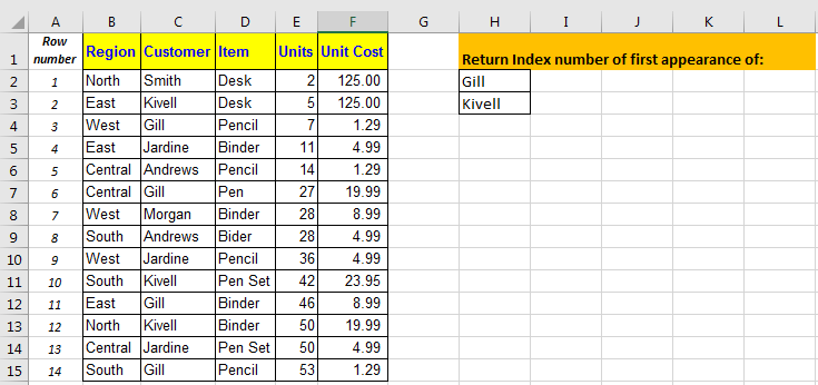
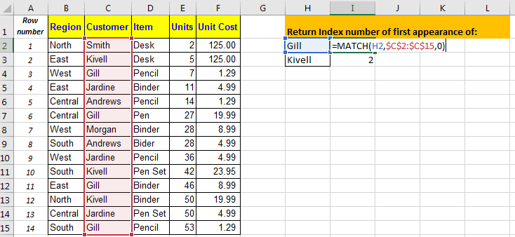
Here In the above image, we have a table. In cell H1, we have our task returning Index number of first appearance of Gill and Kivell.
In cell I2, write this formula and drag it down to I3.
We have our index numbers.
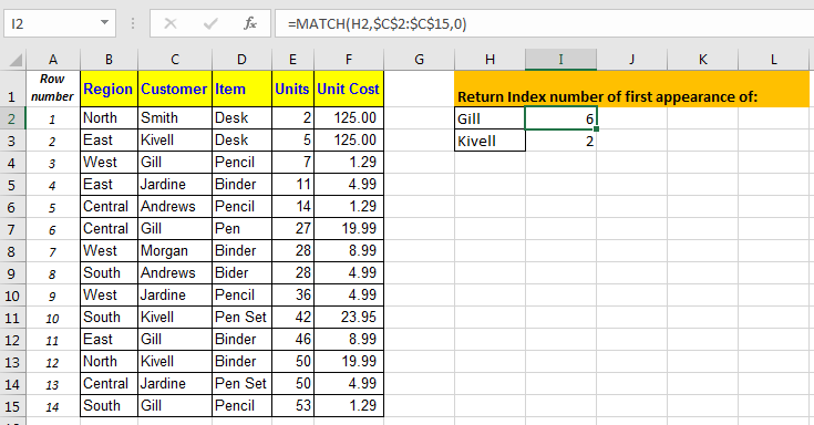
Now you can use this index number with INDEX function of excel to retrieve data from tables.
If you don’t know how to use INDEX MATCH function to retrieve data, below article will be helpful for you.
How to Use Index with Match Function in Microsoft Excel 2010
Do you know how to use the MATCH formula with VLOOKUP to automate reports? In Next article we will learn the use of VLOOKUP MATCH formula. Till then, Keep Practicing — Keep Excelling.
Use of INDEX & MATCH function to lookup value
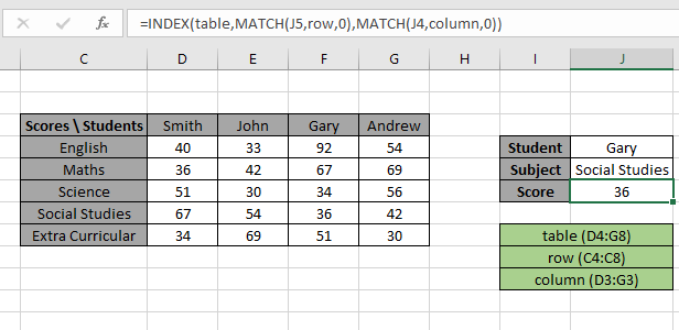
Here we have a list of scores gained by students with their Subject list. We need to find the Score for a specific Student (Gary) & Subject (Social Studies) as shown in the snapshot below.
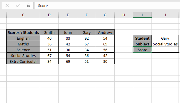
The Student value1 must match the Row_header array and Subject value2 must match the Column_header array.
Use the formula in the J6 cell:
Explanation:
- The MATCH function matches the Student value in J4 cell with the row header array and returns its position 3 as a number.
- The MATCH function matches the Subject value in J5 cell with the column header array and returns its position 4 as a number.
- The INDEX function takes the row and column index number and looks up in the table data and returns the matched value.
- The MATCH type argument is fixed to 0. As the formula will extract the exact match.
Here values to the formula is given as cell references and row_header, table and column_header given as named ranges.
As you can see in the above snapshot, we got the Score obtained by student Gary in Subject Social Studies as 36 . And it proves the formula works fine and for doubts see the below notes for understanding.
Now we will use the approximate match with row headers and column headers as numbers. Approx match only takes the number values as there is no way it applies on text values
Here we have a price of values as per the Height & Width of the product. We need to find the Price for a specific Height (34) & Width (21) as shown in the snapshot below.
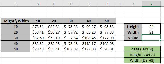
The Height value1 must match the Row_header array and Width value2 must match the Column_header array.
Use the formula in the K6 cell:
Explanation:
- The MATCH function matches the Height value in K4 cell with the row header array and returns its position 3 as a number.
- The MATCH function matches the Width value in K5 cell with the column header array and returns its position 2 as a number.
- The INDEX function takes the row and column index number and looks up in the table data and returns the matched value.
- The MATCH type argument is fixed to 1. As the formula will extract the approximate match.
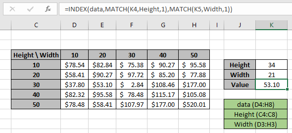
Here values to the formula is given as cell references and row_header, data and column_header given as named ranges as mentioned in the snapshot above.
As you can see in the above snapshot, we got the Price obtained by height (34) & Width (21) as 53.10 . And it proves the formula works fine and for doubts see the below notes for more understanding.
You can also perform lookup exact matches using INDEX and MATCH function in Excel. Learn more about How to do Case Sensitive Lookup using INDEX & MATCH function in Excel. You can also look up for the partial matches using the wildcards in Excel.
Notes:
- The function returns the #NA error if the lookup array argument to the MATCH function is 2 D array which is the header field of the data..
- The function matches the exact value as the match type argument to the MATCH function is 0.
- The lookup values can be given as cell reference or directly using quote symbol ( » ) in the formula as arguments.
Hope this article about How to use the MATCH function in Excel is explanatory. Find more articles on finding values and related Excel formulas here. If you liked our blogs, share it with your friends on Facebook. And also you can follow us on Twitter and Facebook. We would love to hear from you, do let us know how we can improve, complement or innovate our work and make it better for you. Write to us at info@exceltip.com.
Related Articles :
Use INDEX and MATCH to Lookup Value : The INDEX & MATCH formula is used to lookup dynamically and precisely a value in a given table. This is an alternative to the VLOOKUP function and it overcomes the shortcomings of the VLOOKUP function.
Use VLOOKUP from Two or More Lookup Tables : To lookup from multiple tables we can take an IFERROR approach. To lookup from multiple tables, it takes the error as a switch for the next table. Another method can be an If approach.
How to do Case Sensitive Lookup in Excel : The excel’s VLOOKUP function isn’t case sensitive and it will return the first matched value from the list. INDEX-MATCH is no exception but it can be modified to make it case sensitive.
Lookup Frequently Appearing Text with Criteria in Excel : The lookup most frequently appears in text in a range we use the INDEX-MATCH with MODE function.
Popular Articles :
How to use the IF Function in Excel : The IF statement in Excel checks the condition and returns a specific value if the condition is TRUE or returns another specific value if FALSE.
How to use the VLOOKUP Function in Excel : This is one of the most used and popular functions of excel that is used to lookup value from different ranges and sheets.
How to use the SUMIF Function in Excel : This is another dashboard essential function. This helps you sum up values on specific conditions.
How to use the COUNTIF Function in Excel : Count values with conditions using this amazing function. You don’t need to filter your data to count specific values. Countif function is essential to prepare your dashboard.
MATCH in Excel
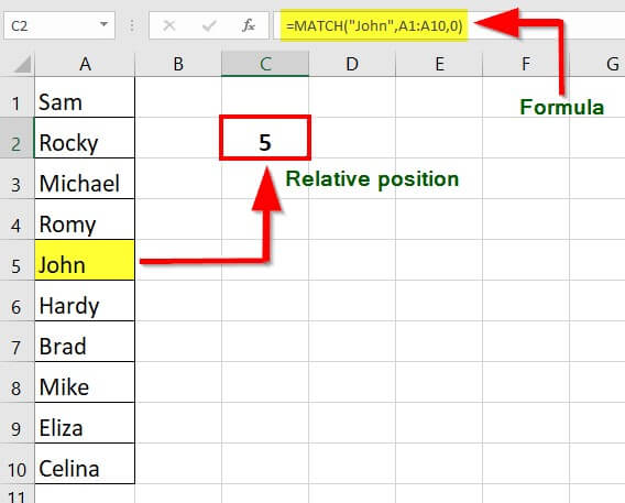
The MATCH function is a powerful tool in Excel that helps users search for a specific value within a range of cells and return its relative position. It’s a useful function for those who work with large datasets or need to locate specific values quickly. For instance, consider a situation where you have a long list of names, and you need to find the position of a particular name (John) within that list. You can use the MATCH function to search for the name and get its position (5).
The utility of the MATCH function extends beyond simple searches within a range. For instance, one can use it in conjunction with other functions like INDEX and OFFSET to perform more complex operations.
Key Highlights
- The MATCH function in Excel can perform both exact and approximate matches.
- It can perform partial matches using wildcard operators such as * and ?.
- The MATCH function returns a #N/A error if it does not find a match in the given array.
- By using the MATCH and INDEX functions together, one can avoid using the VLOOKUP function to find a value at a matched position.
- The Match type is an optional argument in the MATCH function, and if not specified, it defaults to 1.
Syntax of MATCH Function in Excel
The syntax of MATCH function is as follows:
1. Lookup_value (required): Indicates the value whose position we want to find in the selected range. A lookup value can be text, number, logical value, or cell reference.
2. Lookup_array (required): The cell range that contains the lookup value. Lookup array can be a row or a column.
3. Match_Type (optional): An optional argument with values 1, 0, and -1. The match_type argument, set to 0, returns an exact match, while the other two values allow for an approximate match.
a) Match_Type “1”: If the match type value is set as 1, Excel provides a value less than or equal to the lookup value.
b) Match_Type “0”: If the match type value is set as 0, Excel provides the first value that is equal to the lookup value.
c) Match_Type “-1”: If the match type value is set as 0, Excel provides the smallest value that is greater than or equal to the lookup value.
Types of MATCH Function in Excel
You can download this MATCH Function Excel Template here – MATCH Function Excel Template
Here are the different types of MATCH functions in Excel:
#1 Exact MATCH
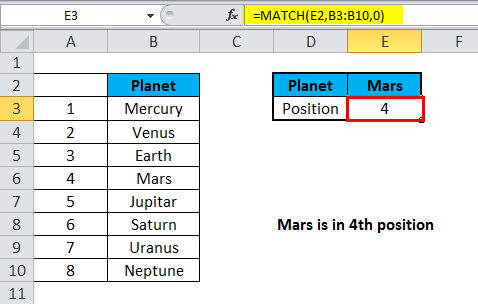
The MATCH function performs an exact match when the match type is set to zero. In the below-given example, the formula in E3 is:
=MATCH(E2,B3:B10,0)
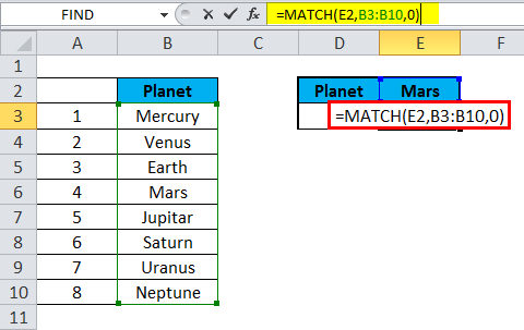
Here, the MATCH Function returns the Exact match as 4.
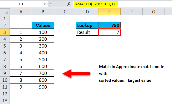
#2 Approximate MATCH
MATCH will perform an approximate match on values sorted A-Z when the match type is set to 1, finding the largest value less than or equal to the lookup value. In the below-given example, the formula in E3 is:
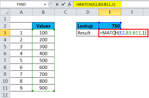
The MATCH in Excel returns an approximate match as 7.
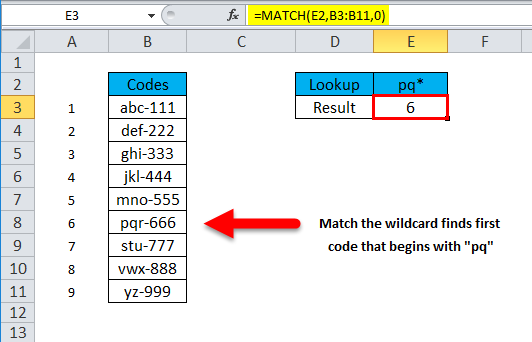
#3 Wildcard MATCH
MATCH function can perform a match using wildcards when the match type is set to zero. In the below-given example, the formula in E3 is:
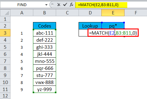
The MATCH function returns the result of wildcards as “pq”.
Points to Note:
- A MATCH Function is not case-sensitive.
- MATCH returns the #N/A error if there is no match is found.
- The argument lookup_array must be in descending order: True, False, Z-A,…9,8,7,6,5,4,3,…, and so on. However, if match_type is set to 1 or omitted, the lookup_array must be sorted in ascending order.
- The wildcard characters like an asterisk () and question mark (?) can be used in the lookup_value argument if match_type is set to 0 and lookup_value is in text format, regardless of whether the lookup_value contains these characters. The asterisk () matches any sequence of characters, while the question mark (?) matches any single character.
How to Use MATCH Function in Excel?
Example #1 Finding The Exact Match
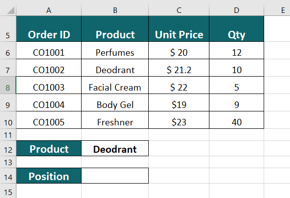
The table below shows a list of ordered products with their order ID, unit price, and sales quantity. We want to find the position of “Deodorant” in the table using the MATCH function in Excel.
Solution:
Step 1: Select the cell where you want to display the position of the product “Deodorant“. In this case, let’s assume it is cell B12.
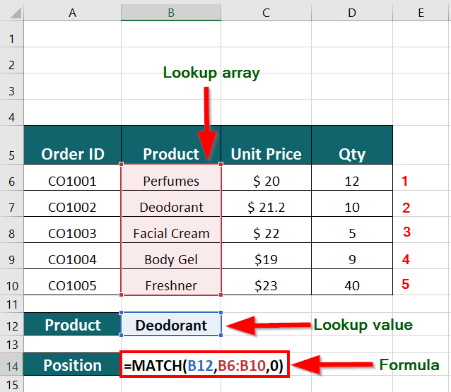
Step 2: Type the MATCH function in the formula bar: =MATCH(B12,B6:B10,0)
- The first argument in the formula is the lookup value, which is “Deodorant“, i.e., cell B12.
- The second argument of the MATCH function is the lookup array, which is the range B6:B10. This range contains the products listed in the table.
Note: The lookup_array can be a row or a column.
- The third argument of the MATCH function is the match type, which is 0. This means we want to find an exact match of the lookup value in the array.
Step 3: Press Enter to get the result, as shown below.
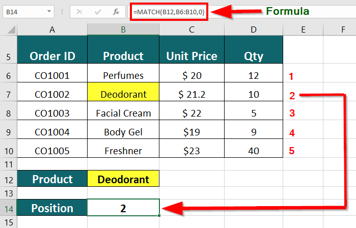
The formula returns the position of “Deodorant” in the table, which is 2. This means that “Deodorant” is the second product listed in the table.
Explanation of the Formula:
When you press the Enter key, Excel searches through the cells in the lookup array “B6:B10” to find an exact match for the lookup value “Deodorant”. After finding the match, it returns the position of the first cell containing the lookup value. In this scenario, the formula returns the value “2“, indicating that the first cell containing “Deodorant” is the second cell in the range B6:B10.
Example #2 Finding Partial MATCH using Wildcard Character
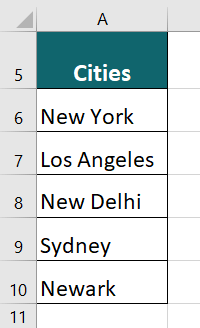
Let’s say we have a list of cities in Column A, and we want to find the position of the city that starts with “New” in the list.
Here’s how we can do it:
Step 1: Open a new Excel spreadsheet and enter the list of cities in Column A.
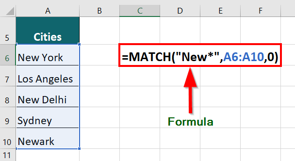
Step 2: In an empty cell, enter the formula =MATCH(“New*”,A6:A10,0).
Explanation of the Formula:
- “New*”: This is the search criteria. The asterisk () is a wildcard character representing any number of characters. So, “New” will match any city name that starts with “New”.
- A6:A10: This is the range of cells we want to search for our city name in.
- 0: This is the match_type argument. Here, we’re using an exact match, so we specify 0.
Step 3: Press the “Enter” key to display the result in the cell where you entered the formula.
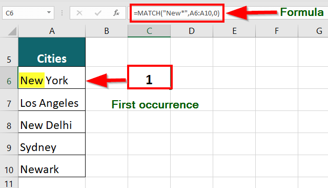
The result is “1,” which is the position of the first city that starts with “New”. In this case, “New York” is the first city that starts with “New” in the list.
Note: If multiple cities match the search criteria, the MATCH function will only return the position of the first occurrence.
Example #3 Using INDEX and MATCH Function Together
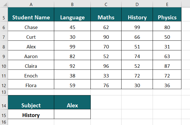
The table below shows a list of students with their marks in the subjects – Language, Maths, History, and Physics. Using the INDEX and MATCH functions together, we want to find Alex’s marks in History
Solution:
Step 1: Select the cell where you want to display the result. In this case, it is cell B15.
Step 2: Enter the formula in the cell:
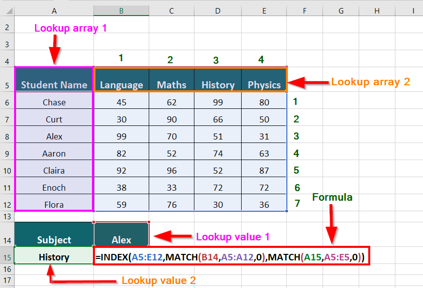
=INDEX(A5:E12,MATCH(B14,A5:A12,0),MATCH(A15,A5:E5,0))
- A5:E12: This is the range of cells containing the table of student data.
- B14: This is the value we want to find in the first column of the table, which is the name of the student whose marks we want to find (in this case, “Alex”).
- A5:A12: This is the range of cells containing the students’ names in the table’s first column.
- 0: This argument specifies that we want an exact match.
- A15: This is the value we’re looking for in row 5, which is the subject “History”.
- A5:E5: This is the cell range containing the subject names.
Step 3: Press Enter key to get the below result.
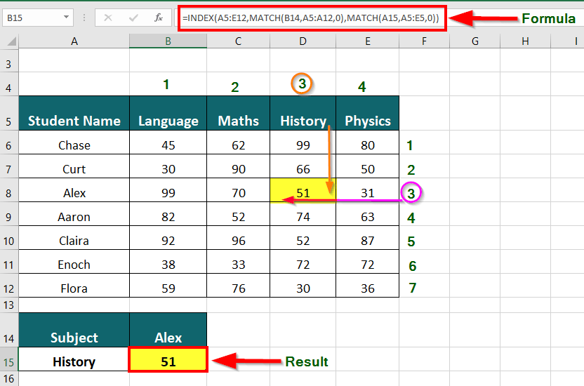
The INDEX and MATCH functions of Excel work together to provide the result of 51, which denote History marks of Alex.
Explanation of the Formula:
- The first MATCH function in the formula =INDEX(A5:E12,MATCH(B14,A5:A12,0),MATCH(A15,A5:E5,0)) searches for the student name “Alex” in the range A5:A12 and returns the relative position of that name within the range. The third argument of the MATCH function is 0, which specifies that we want an exact match. In this case, “Alex” is in the third row of the range, so the first MATCH function returns the value 3.
- The second MATCH function in the formula searches for the subject “History” in the range A5:E5 and returns the relative position of that subject within the range. Again, the third argument of the MATCH function is 0, which specifies that we want an exact match. In this case, “History” is in the third column of the range, so the second MATCH function returns the value 3.
- The INDEX function then uses these two values (3 and 3) to return the corresponding value in the table, which is the marks that Alex scored in History (51).
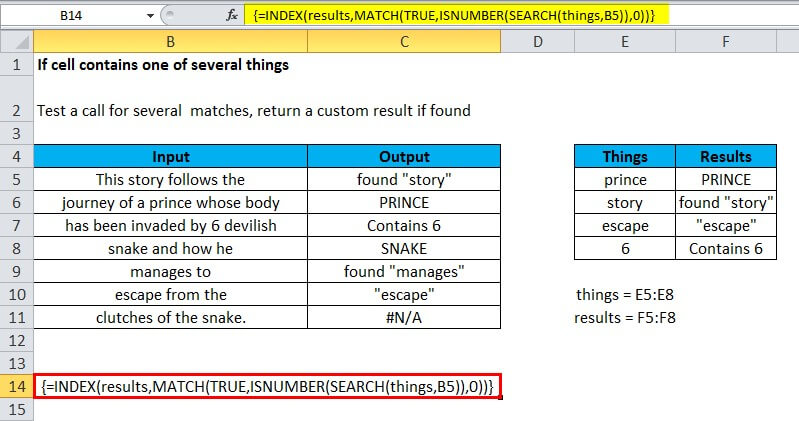
Example #4 When a Cell contains One of Many Things
Generic formula: {=INDEX(results,MATCH(TRUE,ISNUMBER(SEARCH(things,A1)),0))}
Explanation: The INDEX / MATCH function formed on the SEARCH function can be used to check a cell for one of many things and give back a custom result for the first match found.
In the example shown below, the formula in cell C5 is:
{=INDEX(results,MATCH(TRUE,ISNUMBER(SEARCH(things,B5)),0))}
Since the above is an array formula, it should be entered using Control + Shift + Enter keys.
Explanation of the Formula:
- This formula uses two named ranges: E5:E8 is named “things”, and F5:F8 is named “results”.
- Ensure using the name ranges with the same names (depending on the data). If one doesn’t want to use named ranges, use absolute references instead.
- The main part of this formula is the below snippet:
ISNUMBER(SEARCH(things, B5)
- This is based on another formula that checks a cell for a single substring. If the cell has the substring, the formula gives TRUE; if not, the formula gives FALSE
Example #5 Lookup using the Lowest Value
Generic formula =INDEX(range,MATCH(MIN(vals),vals,0))
Explanation: To lookup information associated with the lowest value in a table, one can use a formula depending on MATCH, INDEX, and MIN functions.
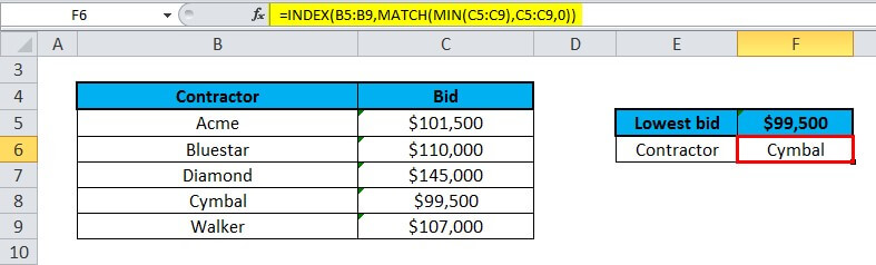
In the below example, a formula is used to find the name of the contractor who has the lowest bid. The formula in F6 is:
=INDEX(B5:B9,MATCH(MIN(C5:C9),C5:C9,0)))
Explanation of the Formula:
- Working from the inside out, the MIN function is generally used to find the lowest bid in the range C5:C9:
- The result, 99500, is fed into the MATCH function as the lookup value:
- MATCH then gives back the position of this value in the range, 4, which goes into INDEX as the row number and B5:B9 as the array:
=INDEX(B5:B9, 4) // returns Cymbal
- The INDEX function then gives back the value at that position: Cymbal.
Match Function Errors
If you get an error from the Match function, this is likely to be the #N/A error:
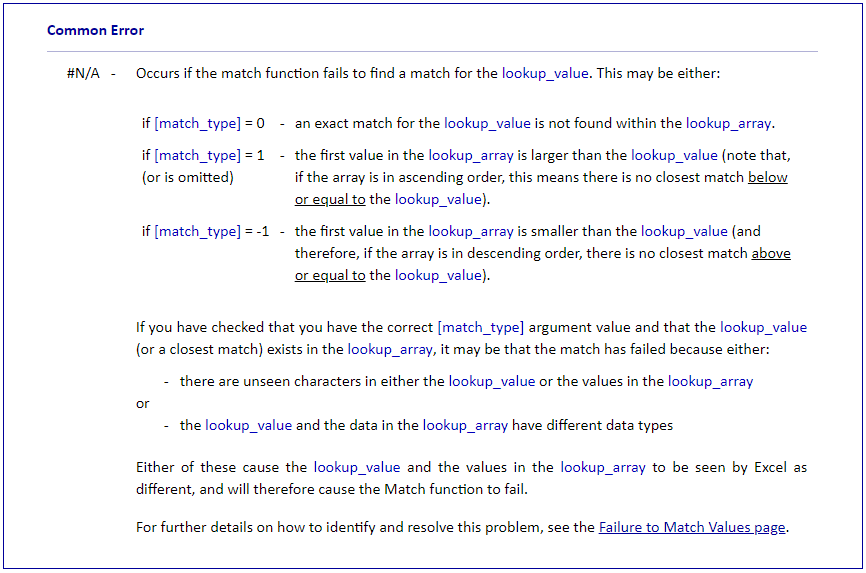
Also, some users experience the following common problem with the Match Function:
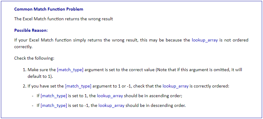
Things to Remember
- MATCH types: One can use three match types with the MATCH function: 0, 1, and -1. The default match type is 0, which finds an exact match. Match type 1 finds the largest value that is less than or equal to the lookup_value, while match type -1 finds the smallest value that is greater than or equal to the lookup_value.
- Array size: The lookup_array argument must be a one-dimensional array or a reference to a one-dimensional range of cells. If the lookup_array is not one-dimensional, the MATCH function will return a #N/A error.
- Sorted order: If the values in the lookup_array are not sorted in ascending order, the MATCH function in Excel may return an incorrect result. In such cases, use the match_type argument to specify the appropriate match type.
- Exact MATCH: If the MATCH function does not find the lookup_value in the lookup_array, it will return a #N/A error. You can use the IFERROR function to handle this error and return a more meaningful result.
- Relative or absolute cell reference: The MATCH function is compatible with both relative and absolute cell references. When copying the formula to other cells, the function will adjust the cell references accordingly.
Frequently Asked Questions (FAQs)
Q1. What is an example of a MATCH function in Excel?
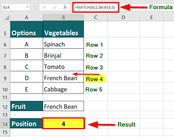
Answer: The MATCH function searches for a given value in a data set and provides the position of that value in the range. For instance, suppose you have a data set that includes items like Spinach, Brinjal, Tomato, French Bean, and Cabbage in the range B6:B10. If you want to find the position of the value “French Bean” in the range, you can use the MATCH function.
The formula =MATCH(B12,B6:B10,0) returns the “French Bean” position in the range B6:B10 as the number 4.
Q2. What is the benefit of including the MATCH function within an INDEX function?
Answer: Including the MATCH function within an INDEX function allows you to retrieve data dynamically based on specific search criteria.
Suppose you have a list of fruits and their prices in a table. You want to retrieve the price of a specific fruit, say “Apple”, from the table. One way to do this is to search the table for the row containing “Apple” manually, and then look for the price in the corresponding column. However, if you have a large dataset with many rows and columns, this can be a time-consuming and error-prone process. Instead, you can use the MATCH function to find the row number of “Apple” in the table and then use the INDEX function to retrieve the price from the corresponding column. The formula would look like this:
=INDEX(B2:E6,MATCH(“Apple”,A2:A6,0),3)
The MATCH function searches for “Apple” in the table’s first column (A2:A6) and returns the row number where it is found. The INDEX function then retrieves the value from the table’s third column (price column) at the intersection of the row and column numbers that the MATCH function returns.
Q3. Can the MATCH function have multiple criteria?
Answer: It is possible to use the MATCH function with multiple criteria by combining it with other functions such as INDEX, SUMPRODUCT, and COUNTIFS. For instance, consider this formula:
= MATCH(1, (B2:B10=”Sales”) * (C2:C10>20000), 0) + COUNTIFS(B2:B10, “Sales”, C2:C10, “>20000”)
This formula uses MATCH with multiple criteria to find the position of the first employee in the “Sales” department who earns more than $20,000 per year. Then, it adds the count of cells that satisfy only the second condition using the COUNTIFS function.
Q4. What is the difference between MATCH and VLOOKUP in Excel?
Answer: The MATCH function helps us find the location of a particular value in a column or row, while the VLOOKUP function helps us retrieve information associated with that value.
For instance, if we want to find the price of oranges in the following table, we will have to use the MATCH function in conjunction with the INDEX function to find the price. Alternatively, the VLOOKUP function can directly provide the price of oranges at $0.75.
|
Product |
Price |
| Apples | $1.00 |
| Oranges | $0.75 |
| Bananas | $0.50 |
The formula for using MATCH and INDEX functions together is =INDEX(B:B, MATCH(“Oranges”, A:A, 0)). Using MATCH, this formula finds the position of “Oranges” in column A, which returns the value 2. Then, INDEX retrieves the value in column B’s corresponding row, i.e., $0.75.
- The VLOOKUP function formula is =VLOOKUP(“Oranges”, A:B, 2, 0). This formula looks for “Oranges” in the first column of the range A:B, and returns the corresponding value from the second column (i.e., the price column), resulting in $0.75.
Recommended Articles
The above article is our guide to using the MATCH function in Excel. Here are some further examples of expanding understanding:
- Excel Match Multiple Criteria
- How to Match Data in Excel
- Matching Columns in Excel
- Compare Two Columns in Excel for Matches
Excel provides many formulas for finding a particular string or text in an array. One such function is MATCH, in fact Match function is designed to do a lot more than this. Today we are going to learn how to use the Excel Match function. Basically what match function does is, it scans the whole array range in order to find the specified text and thereafter it returns its position.
Excel Match Function Definition:
Excel defines match function as: “Returns the relative position of an item in an array that matches a specified value in a specified order”. In simple plain language Match function searches for a value in a defined range and then returns its position.
Syntax of Match Formula:
Match formula can be written as: MATCH(lookup_value, range, match_type)
Here: ‘lookup_value’ signifies the value to be searched in the array.
‘range’ is the array of values on which you want to perform a match.
‘match_type’ Match type is an important thing. It can have three values 1, 0 or -1.
- If ‘match_type’ has a value 1, it means that match function will find a value that is less than or equal to ‘lookup_value’. It can only be applied if the array (‘range’) is sorted in an ascending order.
- If ‘match_type’ has a value 0, it means that match function will find the first value that is equal to the ‘lookup_value’. In this case sorting of array (‘range’) is not important.
- If ‘match_type’ has a value -1, it means that match function will find the smallest value that is greater than or equal to ‘lookup_value’. It can only be applied if the array (‘range’) is sorted in a descending order.
Few Important things about Match Formula:
- Match is case-insensitive. It does not know the difference between upper and lower case.
-
If ‘match_type’ i.e. the third parameter of match function is omitted, then the function treats its value to be 1 as default.
-
If the Match formula cannot find any matches, it results into #N/A error.
-
Match function also supports the use of wildcard operators, but they can only be used in case of text comparisons where the ‘match_type’ is 0. We will cover this with an example later.
-
Match function does not return the matching string, it only returns the relative position of that string.
-
If the array is not sorted in the ascending order for ‘match_type’ 1 then it results into a #N/A error. Similarly #N/A error also occurs if the defined cell range is not sorted in descending order for ‘match_type’ equal to -1.
Example of Match Formula in Excel:

- In the first example we have applied a Match function as shown in the above image.
The Match Function is applied as: =MATCH(104,B2:B8,1)
The Result is 3.
This means that Match searches the whole range for the value 104 but as 104 was not present in the list so it pointed to the relative position of a value slightly less than 104 i.e. 103. If in the same example the array would have the value 104 with array being sorted in ascending order then the same formula would have resulted into pointing the relative reference of 104.
- If we apply another Match function:
=MATCH(104,B2:B8,0)on the same data set.
Then it will result into an error as ‘0’ signifies exact match and in absence of the value 104 the function will give an error #N/A
- If we apply another Match function:
=MATCH(104,B2:B8,-1)on the same data set.
Then it will result into an error as the array is not sorted in descending order.

- In the second example a Match formula with match type as -1 is used.
The Result is: 4
This is because as the value 104 is not present in the array so the Match function points to the relative reference of a value slightly greater than 104 i.e. 105.
WildCard Operators in Match Function:
Using wildcards can only prove useful in the case of exact string matches i.e. ‘match_type’ 0. Generally two types of wildcard operators can be used within the Match Function.
- “?” Wildcard: This signifies any single character.
-
“*” Wildcard: This signifies any number of characters.

In the above example we have applied a Match Formula as: =MATCH("T?a",A2:A8,0)
The ‘lookup_value’ contains the “?” wildcard operator which matches the array element “Tea” and hence the result of match function is the relative position of “Tea” i.e. 3
If another Match function: =MATCH("C*e",A2:A8,0) is applied on the same dataset. Then it will result into a value 7. As “C*e” matches “coffee” and hence the Match function gives the relative position of “Coffee” element in the array.
So, this was all about Match function in Excel. Do let me know if you have any queries about this wonderful function.
На чтение 2 мин
Функция ПОИСКПОЗ в Excel используют для поиска точной позиции искомого значения в списке или массиве данных.
Содержание
- Что возвращает функция
- Синтаксис
- Аргументы функции
- Дополнительная информация
- Примеры использования функции ПОИСКПОЗ в Excel
Что возвращает функция
Возвращает число, соответствующее позиции искомого значения.
 Больше лайфхаков в нашем Telegram Подписаться
Синтаксис
=MATCH(lookup_value, lookup_array, [match_type]) — английская версия
=ПОИСКПОЗ(искомое_значение;просматриваемый_массив;[тип_сопоставления]) — русская версия
Аргументы функции
- lookup_value (искомое_значение) — значение, с которым вы хотите сопоставить данные из массива или списка данных;
- lookup_array (просматриваемый_массив) — диапазон ячеек в котором вы осуществляете поиск искомых данных;
- [match_type] ([тип_сопоставления]) — (не обязательно) — этот аргумент определяет каким образом, будет осуществлен поиск. Допустимые значения для аргумента: «-1», «0», «1» (подробней читайте ниже).
Дополнительная информация
- Чаще всего функция MATCH используется в сочетании с функцией INDEX (ИНДЕКС);
- Подстановочные знаки могут использоваться в аргументах функции в тех случаях, когда значение поиска — текстовая строка;
- При использовании функции ПОИСКПОЗ регистр букв не учитывается;
- Функция возвращает #N/A ошибку, если искомое значение не найдено;
- Аргумент match_type (тип_сопоставления) определяет каким образом, будет осуществлен поиск:
— Если аргумент match_type (тип_сопоставления) = 0, то это критерий точного соответствия. Он возвращает первую точную позицию соответствия (или ошибку, если совпадения нет);
— Если аргумент match_type (тип_сопоставления) = 1 (по умолчанию), то в таком случае данные должны быть отсортированы в порядке возрастания для этой опции. Функция возвращает наибольшее значение, равное или меньшее значения поиска.
— Если аргумент match_type (тип_сопоставления) = -1, то в таком случае данные должны быть отсортированы в порядке убывания для этой опции. Функция возвращает наименьшее и наибольшее значения поиска.
Примеры использования функции ПОИСКПОЗ в Excel
The MATCH function looks for a specific value and returns its relative position in a given range of cells. The output is the first position found for the given value. Being a lookup and reference function, it works for both an exact and approximate match. For example, if the range A11:A15 consists of the numbers 2, 9, 8, 14, 32, the formula “MATCH(8,A11:A15,0)” returns 3. This is because the number 8 is at the third position.
In simple words, the MATCH formula is given as follows:
“MATCH(value to be searched, array, exact or approximate match [1, 0 or -1])”
Table of contents
- MATCH Function in Excel
- The Syntax of the MATCH Excel Function
- How to use the MATCH Function in Excel? (With Examples)
- Example #1–Exact Match
- Example #2–Approximate Match
- Example #3–Wildcard Character (Partial Match)
- Example 4–INDEX MATCH
- The Properties of the MATCH Excel Function
- Frequently Asked Questions
- Recommended Articles
The Syntax of the MATCH Excel Function
The syntax of the function is shown in the following image:

The function accepts the following arguments:
- Lookup_value: This is the value to be searched in the “lookup_array.”
- Lookup_array: This is the array or range of cells where the “lookup_value” is to be searched.
- Match_type: This takes the values 1, 0, or -1 depending on the type of match.
For instance, you may want to search a specific word (lookup_value) in the dictionary (lookup_array).
The arguments “lookup_value” and “lookup_array” are mandatory, while “match_type” is optional.
The Values of “Match_Type”
The “match_type” can take any of the following values:
Positive one (1): The function looks for the largest value in the “lookup_array,” which is less than or equal to the “lookup_value.” The data is arranged in alphabetical (A to Z) or ascending order and an approximate match is returned.
Zero (0): The function looks for an exact match of the “lookup_value” in the “lookup_array.” The data is not required to be arranged.
Negative one (-1): The function looks for the smallest value in the “lookup_array,” which is greater than or equal to the “lookup_value.” The data is arranged in reverse order of alphabets (Z to A) or descending order and an approximate match is returned.
Note: The default value of “match_type” is 1.
How to use the MATCH Function in Excel? (With Examples)
Let us understand the working of the MATCH formula with the help of examples.
You can download this MATCH Function Excel Template here – MATCH Function Excel Template
Example #1–Exact Match
The succeeding table shows the serial number (S.N.), name, and department of ten employees in an organization. We want to find the position of the employee “Tanuj.”
We apply the following formula.
“=MATCH(F4,$B$4:$B$13,0)”
The “match_type” is set at 0 to return the exact position of “Tanuj” (lookup_value) from the range $B$4:$B$13 (lookup_array). The output is 1.

Example #2–Approximate Match
The succeeding list shows the values from 100 to 1000. We want to find the approximate position of the value 525.
We apply the following formula.
“=MATCH(E19,B19:B28,1)”
The “match_type” is set at 1 to return the approximate match of 525 (lookup_value) from the range B19:B28 (lookup_array).
The MATCH function looks for the largest value (500), which is less than 525 in the given array. Hence, the output is 5.

Example #3–Wildcard Character (Partial Match)
The MATCH function supports the usage of wildcard charactersIn Excel, wildcards are the three special characters asterisk, question mark, and tilde. Asterisk denotes multiple characters, a question mark denotes a single character, and a tilde denotes the identification of a wild card character.read more (? and *) in the “lookup_value” argument. Let us consider an example of the same.
The succeeding list shows ten IDs of the various employees of an organization. We want to find the position of the ID ending with 105.
We apply the following formula.
“=MATCH(“*”&E33,$B$33:$B$42,0)”
The wildcard characters are used for partial matches and the “match_type” is set at zero. The output is 5. This implies that the ID at the fifth position is ending with 105.

Example 4–INDEX MATCH
The MATCH and INDEX functionThe INDEX function can return the result from the row number, and the MATCH function can give us the position of the lookup value in the array. This combination of the INDEX MATCH is beneficial in addressing a fundamental limitation of VLOOKUP.read more are used together to look up a value in the table from right to left.
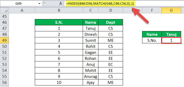
The succeeding table shows the serial number (S.N.), name, and department of ten employees in an organization. We want to find the serial number of the employee “Tanuj.”
We apply the following formula.
“=INDEX(B46:D56,MATCH(G48,C46:C56,0),1)”
The MATCH function searches for the exact word “Tanuj” in the range C46:C56 and returns 2. The output 2 is supplied as the row number to the INDEX functionThe INDEX function in Excel helps extract the value of a cell, which is within a specified array (range) and, at the intersection of the stated row and column numbers.read more. The INDEX function returns the value from the second row and first column of the range B46:D56.
The output of the formula is 1. This implies that the serial number of “Tanuj” is 1.
The following image shows the output when the “lookup_value” is “Tanujh.” Since “Tanujh” could not be found in column B, the outcome is “#N/A” error.

The Properties of the MATCH Excel Function
- It is not case-sensitive which implies that it does not distinguish between the uppercase and lowercase letters.
- It returns the relative position of the “lookup_value” in the “lookup_array.”
- It works with one-dimensional ranges or arrays which can be either vertical or horizontal.
- If there are multiple occurrences of the “lookup_value” in the “lookup_array,” it returns the position of the first exact match.
- If the “lookup_value” is in text form, the wildcard characters like a question mark (?) and asterisk (*) can be used for partial matches.
- It returns the “#N/A” error if it is unable to find the “lookup_value” in the “lookup_array.”
Frequently Asked Questions
1. Define the MATCH function of Excel.
The MATCH function returns the position of a given value from a vertical or horizontal array or range of cells. It returns both approximate and exact matches from unsorted and sorted data lists respectively.
The MATCH function can be used in combination with the INDEX function to extract a value from the position supplied by the former. The MATCH function accepts the arguments “lookup_value,” “lookup_array,” and “match_type.”
The first two arguments are mandatory, while the last is optional. The “match_type” can take the values 1, 0 or -1 depending on the type of match. The value 0 refers to an exact match, while 1 and -1 refer to an approximate match.
2. How is the MATCH function used to compare two columns in Excel?
The MATCH function is used in combination with the IF and ISNA functions to compare two columns. The formula is stated as follows:
“IF(ISNA(MATCH(first value in list1,list2,0)),“not in list 1”,“”)”
The formula looks for a value of “list 1” in “list 2.” If it is able to find a value, its relative position is returned. However, if a value of “list 2” is not present in “list 1,” the formula returns the text “not in list 1.”
3. What is the INDEX MATCH formula of Excel?
The INDEX MATCH formula uses a combination of the INDEX and MATCH functions. The INDEX function looks for a value in an array based on the specified row and column numbers. These row and column numbers are supplied by the MATCH function.
The INDEX MATCH formula for a vertical lookup is stated as follows:
“INDEX(column to return a value from,MATCH(lookup_value,column to look up against,0)”
The “column to return a value from” is the “array” argument of the INDEX function. The “column to look up against” is the “lookup_array” argument of the MATCH function.
Note: The “array” argument of the INDEX function must contain the same number of rows as the “lookup_array” argument of the MATCH function.
Recommended Articles
This has been a guide to the MATCH function in excel. Here we discuss how to use Match Formula along with step by step excel example. You can download the Excel template from the website. Take a look at these lookup and reference functions of Excel-
- Excel Match Multiple CriteriaCriteria based calculations in excel are performed by logical functions. To match single criteria, we can use IF logical condition, having to perform multiple tests, we can use nested IF conditions. But for matching multiple criteria to arrive at a single result is a complex criterion-based calculation.read more
- Excel Mathematical FunctionMathematical functions in excel refer to the different expressions used to apply various forms of calculation. The seven frequently used mathematical functions in MS excel are SUM, AVERAGE, AVERAGEIF, COUNTA, COUNTIF, MOD, and ROUND.read more
- INDEX FormulaThe INDEX function in Excel helps extract the value of a cell, which is within a specified array (range) and, at the intersection of the stated row and column numbers.read more
- VBA MatchIn VBA, the match function is used as a lookup function and is accessed by the application. worksheet method. The arguments for the Match function are similar to the worksheet function.read more