
The INDEX function returns a value or the reference to a value from within a table or range.

There are two ways to use the INDEX function:
-
If you want to return the value of a specified cell or array of cells, see Array form.
-
If you want to return a reference to specified cells, see Reference form.
Array form
Description
Returns the value of an element in a table or an array, selected by the row and column number indexes.
Use the array form if the first argument to INDEX is an array constant.
Syntax
INDEX(array, row_num, [column_num])
The array form of the INDEX function has the following arguments:
-
array Required. A range of cells or an array constant.
-
If array contains only one row or column, the corresponding row_num or column_num argument is optional.
-
If array has more than one row and more than one column, and only row_num or column_num is used, INDEX returns an array of the entire row or column in array.
-
-
row_num Required, unless column_num is present. Selects the row in array from which to return a value. If row_num is omitted, column_num is required.
-
column_num Optional. Selects the column in array from which to return a value. If column_num is omitted, row_num is required.
Remarks
-
If both the row_num and column_num arguments are used, INDEX returns the value in the cell at the intersection of row_num and column_num.
-
row_num and column_num must point to a cell within array; otherwise, INDEX returns a #REF! error.
-
If you set row_num or column_num to 0 (zero), INDEX returns the array of values for the entire column or row, respectively. To use values returned as an array, enter the INDEX function as an array formula.
Note: If you have a current version of Microsoft 365, then you can input the formula in the top-left-cell of the output range, then press ENTER to confirm the formula as a dynamic array formula. Otherwise, the formula must be entered as a legacy array formula by first selecting the output range, input the formula in the top-left-cell of the output range, then press CTRL+SHIFT+ENTER to confirm it. Excel inserts curly brackets at the beginning and end of the formula for you. For more information on array formulas, see Guidelines and examples of array formulas.
Examples
Example 1
These examples use the INDEX function to find the value in the intersecting cell where a row and a column meet.
Copy the example data in the following table, and paste it in cell A1 of a new Excel worksheet. For formulas to show results, select them, press F2, and then press Enter.
|
Data |
Data |
|
|---|---|---|
|
Apples |
Lemons |
|
|
Bananas |
Pears |
|
|
Formula |
Description |
Result |
|
=INDEX(A2:B3,2,2) |
Value at the intersection of the second row and second column in the range A2:B3. |
Pears |
|
=INDEX(A2:B3,2,1) |
Value at the intersection of the second row and first column in the range A2:B3. |
Bananas |
Example 2
This example uses the INDEX function in an array formula to find the values in two cells specified in a 2×2 array.
Note: If you have a current version of Microsoft 365, then you can input the formula in the top-left-cell of the output range, then press ENTER to confirm the formula as a dynamic array formula. Otherwise, the formula must be entered as a legacy array formula by first selecting two blank cells, input the formula in the top-left-cell of the output range, then press CTRL+SHIFT+ENTER to confirm it. Excel inserts curly brackets at the beginning and end of the formula for you. For more information on array formulas, see Guidelines and examples of array formulas.
|
Formula |
Description |
Result |
|---|---|---|
|
=INDEX({1,2;3,4},0,2) |
Value found in the first row, second column in the array. The array contains 1 and 2 in the first row and 3 and 4 in the second row. |
2 |
|
Value found in the second row, second column in the array (same array as above). |
4 |
|
Top of Page
Reference form
Description
Returns the reference of the cell at the intersection of a particular row and column. If the reference is made up of non-adjacent selections, you can pick the selection to look in.
Syntax
INDEX(reference, row_num, [column_num], [area_num])
The reference form of the INDEX function has the following arguments:
-
reference Required. A reference to one or more cell ranges.
-
If you are entering a non-adjacent range for the reference, enclose reference in parentheses.
-
If each area in reference contains only one row or column, the row_num or column_num argument, respectively, is optional. For example, for a single row reference, use INDEX(reference,,column_num).
-
-
row_num Required. The number of the row in reference from which to return a reference.
-
column_num Optional. The number of the column in reference from which to return a reference.
-
area_num Optional. Selects a range in reference from which to return the intersection of row_num and column_num. The first area selected or entered is numbered 1, the second is 2, and so on. If area_num is omitted, INDEX uses area 1. The areas listed here must all be located on one sheet. If you specify areas that are not on the same sheet as each other, it will cause a #VALUE! error. If you need to use ranges that are located on different sheets from each other, it is recommended that you use the array form of the INDEX function, and use another function to calculate the range that makes up the array. For example, you could use the CHOOSE function to calculate which range will be used.
For example, if Reference describes the cells (A1:B4,D1:E4,G1:H4), area_num 1 is the range A1:B4, area_num 2 is the range D1:E4, and area_num 3 is the range G1:H4.
Remarks
-
After reference and area_num have selected a particular range, row_num and column_num select a particular cell: row_num 1 is the first row in the range, column_num 1 is the first column, and so on. The reference returned by INDEX is the intersection of row_num and column_num.
-
If you set row_num or column_num to 0 (zero), INDEX returns the reference for the entire column or row, respectively.
-
row_num, column_num, and area_num must point to a cell within reference; otherwise, INDEX returns a #REF! error. If row_num and column_num are omitted, INDEX returns the area in reference specified by area_num.
-
The result of the INDEX function is a reference and is interpreted as such by other formulas. Depending on the formula, the return value of INDEX may be used as a reference or as a value. For example, the formula CELL(«width»,INDEX(A1:B2,1,2)) is equivalent to CELL(«width»,B1). The CELL function uses the return value of INDEX as a cell reference. On the other hand, a formula such as 2*INDEX(A1:B2,1,2) translates the return value of INDEX into the number in cell B1.
Examples
Copy the example data in the following table, and paste it in cell A1 of a new Excel worksheet. For formulas to show results, select them, press F2, and then press Enter.
|
Fruit |
Price |
Count |
|---|---|---|
|
Apples |
$0.69 |
40 |
|
Bananas |
$0.34 |
38 |
|
Lemons |
$0.55 |
15 |
|
Oranges |
$0.25 |
25 |
|
Pears |
$0.59 |
40 |
|
Almonds |
$2.80 |
10 |
|
Cashews |
$3.55 |
16 |
|
Peanuts |
$1.25 |
20 |
|
Walnuts |
$1.75 |
12 |
|
Formula |
Description |
Result |
|
=INDEX(A2:C6, 2, 3) |
The intersection of the second row and third column in the range A2:C6, which is the contents of cell C3. |
38 |
|
=INDEX((A1:C6, A8:C11), 2, 2, 2) |
The intersection of the second row and second column in the second area of A8:C11, which is the contents of cell B9. |
1.25 |
|
=SUM(INDEX(A1:C11, 0, 3, 1)) |
The sum of the third column in the first area of the range A1:C11, which is the sum of C1:C11. |
216 |
|
=SUM(B2:INDEX(A2:C6, 5, 2)) |
The sum of the range starting at B2, and ending at the intersection of the fifth row and the second column of the range A2:A6, which is the sum of B2:B6. |
2.42 |
Top of Page
See Also
VLOOKUP function
MATCH function
INDIRECT function
Guidelines and examples of array formulas
Lookup and reference functions (reference)
![]()
Download Article
![]()
Download Article
If your Excel workbook contains numerous worksheets, you can add a table of contents that indexes all of your sheets with clickable hyperlinks. This tutorial will teach you how to make an index of sheet names with page numbers in your Excel workbook without complicated VBA scripting, and how to add helpful «back to index» buttons to each sheet to improve navigation.
-

1
Create an index sheet in your workbook. This sheet can be anywhere in your workbook, but you’ll usually want to place the tab at the beginning like a traditional table of contents.
- To create a new sheet, click the + at the bottom of the active worksheet. Then, right-click the new tab, select Rename, and type a name for your sheet like Index or Worksheets.
- You can rearrange sheets by dragging their tabs left or right at the bottom of your workbook.
-
2
Type Page Number into cell A1 of your index sheet. Column A is where you’ll be placing the page numbers for each sheet.
Advertisement
-
3
Type Sheet Name into cell B1 of your index sheet. This will be the column header above your list of worksheets.
-
4
Type Link into cell C1 of your index sheet. This is the column header that will appear above hyperlinks to each worksheet.
-
5
Click the Formulas tab. It’s at the top of Excel.
-
6
Click Define Name. It’s on the «Defined Names» tab at the top of Excel.
-
7
Type SheetList into the «Name» field. This names the formula you’ll be using with the INDEX function.[1]
-
8
Type the formula into the «Refers to» field and click OK. The formula is =REPLACE(GET.WORKBOOK(1),1,FIND("]",GET.WORKBOOK(1)),"").
-
9
Enter page numbers in column A. This is the only part you’ll have to do manually. For example, if your workbook has 20 pages, you’ll type 1 into A2, 2 into A3, etc., and continue numbering down until you’ve entered all 20 page numbers.
- To quickly populate the page numbers, type the first two page numbers into A2 and A3, click A3 to select it, and then drag the square at A3’s bottom-right corner down until you’ve reached the number of pages in your workbook. Then, click the small icon with a + that appears at the bottom-right corner of the column and select Fill Series.
-
10
Type this formula into cell B2 of your index sheet. The formula is =INDEX(SheetList,A2). When you press Enter or Return, you’ll see the name of the first sheet in your workbook.
-
11
Fill the rest of column B with the formula. To do this, just click B2 to select it, and then double-click the square at its bottom-right corner. This adds the name of each worksheet corresponding to the page numbers you typed into column A.
-
12
Type this formula into C2 of your worksheet. The formula is =HYPERLINK("#'"&B2&"'!A1","Go to Sheet"). When you press Enter or Return, you’ll see a hyperlink to the first page in your index called «Go to Sheet.»
-
13
Fill the rest of column C with the formula. To do this, click C2 to select it, and then double-click the square at its bottom-right corner. Now each sheet in your workbook has a clickable hyperlink that takes you right to that page.
-
14
Save your workbook in the macro-enabled format. Because you created a named range, you’ll need to save your workbook in this format.[2]
Here’s how:- Go to File > Save.
- On the pop-up message that warns you about saving a macro-free workbook, click No.
- In the «Save as type» or file format menu, select Excel Macro-Enabled Workbook (*.xlsm) and click Save.


Advertisement
-
1
Click your index or table of contents sheet. If you have a lot of pages in your workbook, it’ll be helpful to readers to add quick «Back to Index» or «Back to Table of Contents» links to each sheet so they don’t have to scroll through lots of worksheet tabs after clicking to that page. Start by opening your index sheet.
-
2
Name the index. To do this, just click the field directly above cell A1, type Index, and then press Enter or Return.
- Don’t worry if the field already contains a cell address.
-
3
Click any of the sheets in your workbook. Now you’ll create your back button. Once you create a back button on one sheet, you can just copy and paste it onto other sheets.
-
4
Click the Insert tab. It’s at the top of the screen.
-
5
Click the Illustrations menu and select Shapes. This option will be in the upper-left area of Excel.
-
6
Click a shape for your button. For example, if you want to create a back-arrow icon sort of like your web browser’s back button, you can click the left-pointing arrow under the «Block Arrows» header.
-
7
Click the location where you want to place the button. Once you click, the shape will appear. If you want, you can change the color and look using the options at the top, and/or resize the shape by dragging any of its corners.
-
8
Type some text onto the shape. The text you type should be something like «Back to Index.» You can double-click the shape to place the cursor and start typing right onto the actual shape
- You might need to drag the corner of the shape to resize it so the text fits.
- To place a text box on or near the shape before typing, just click the Shape Format menu at the top (while the shape is selected), click Text Box in the toolbar, and then click and drag a text box.
- You can stylize the text using the options in Text on the toolbar while the shape is selected.
-
9
Right-click the shape and select Link. This opens the Insert Hyperlink dialog.[3]
-
10
Click the Place in This Document icon. It’s in the left panel.
-
11
Select your index under «Defined Names» and click OK. You might have to click the + next to the column header to see the Index option. This makes the text in the shape a clickable hyperlink that takes you right to the index.
-
12
Copy and paste the hyperlink to other sheets. To do this, just right-click the shape and select Copy. Then, you can paste it onto any other page by right-clicking the desired location and selecting the first icon under «Paste Options» (the one that says «Use Destination Theme» when you hover the mouse over it).


Advertisement
Ask a Question
200 characters left
Include your email address to get a message when this question is answered.
Submit
Advertisement
Thanks for submitting a tip for review!
About This Article
Article SummaryX
To create a table of contents in Excel, you can use the «Defined Name» option to create a formula that indexes all sheet names on a single page. Then, you can use the INDEX function to list the sheet names, as well as the HYPERLINK function to create quick links to each sheet.
Did this summary help you?
Thanks to all authors for creating a page that has been read 55,649 times.
Is this article up to date?
#1 How to Use the INDEX Formula
- Type “=INDEX(” and select the area of the table, then add a comma.
- Type the row number for Kevin, which is “4,” and add a comma.
- Type the column number for Height, which is “2,” and close the bracket.
- The result is “5.8.”
Contents
- 1 How do you create an index in Excel?
- 2 How do I index a column in Excel?
- 3 How do you enter an index?
- 4 What is an Excel INDEX?
- 5 What is a INDEX sheet?
- 6 How do I find the index of a column?
- 7 How do I create an Index in notebook?
- 8 Where is the Index page of a document found?
- 9 How do you write an Index for a project?
- 10 How do I create an index link in Excel?
- 11 How do I index another sheet in Excel?
- 12 How do you create an index score?
- 13 What is an index column?
- 14 How do you find the index of a data frame?
- 15 How do you set an index for a data frame?
- 16 What is the meaning of index in notebook?
- 17 How do you make a bullet Journal from scratch?
- 18 What pages do you need in a bullet Journal?
- 19 How do I index a Word document?
- 20 How do you create an index table in Word?
How do you create an index in Excel?
An index column is also added to an Excel worksheet when you load it. To open a query, locate one previously loaded from the Power Query Editor, select a cell in the data, and then select Query > Edit. For more information see Create, load, or edit a query in Excel (Power Query). Select Add Column > Index Column.
How do I index a column in Excel?
MATCH Function to get Column Index from Table 1
- Select cell H3 and click on it.
- Insert the formula: =MATCH(G3,Table1[#Headers],0)
- Press enter.
- Drag the formula down to the other cells in the column by clicking and dragging the little “+” icon at the bottom-right of the cell.
How do you enter an index?
Insert an Index Entry
- Select the text you want to include in the index.
- Click the References tab.
- Click the Mark Entry in the Index group.
- Adjust the index entry’s settings and choose an index entry option:
- Click the Mark or Mark All button.
- Repeat the process for your other index entries.
- Click Close when you’re done.
What is an Excel INDEX?
Summary. The Excel INDEX function returns the value at a given location in a range or array. You can use INDEX to retrieve individual values, or entire rows and columns. The MATCH function is often used together with INDEX to provide row and column numbers.
What is a INDEX sheet?
The INDEX function in Google Sheets returns the value of a cell within an input range, relatively separated from the first cell by row and column offsets. This is similar to the index at the end of a book, which provides a quick way to locate specific content.
How do I find the index of a column?
Get column index from column name of a given Pandas DataFrame
- Syntax: DataFrame.columns.
- Return: column names index.
- Syntax: Index.get_loc(key, method=None, tolerance=None)
- Return: loc : int if unique index, slice if monotonic index, else mask.
How do I create an Index in notebook?
Setting up your Index is easy. Simply leave the first couple pages of your notebook blank and give them the topic of “Index.” As you start to use your book, add the topics of your entries and their page numbers to the Index, so you can quickly find your them later.
Where is the Index page of a document found?
What Is An Index? An index is an alphabetical and detailed listing of topics in a document, with a corresponding page number displayed alongside (see picture below). An index is typically located at the end of a long document.
How do you write an Index for a project?
Guide to the Project Index
- Client Name/Project Name: The first column lists the Client or Project name.
- Location and State: The geographical location of the project.
- Date: The date of the project.
- Project Type: The general term for the category of building.
- Collaborator/Role:
- Physical Location of Materials:
- Microfilm:
How do I create an index link in Excel?
Simply select the cell, and then Insert > Hyperlink. This brings up the Insert Hyperlink dialog box, pictured below. To set up a link to another sheet or named reference within the workbook, simply click Place in This Document from the Link to panel.
How do I index another sheet in Excel?
How to reference another sheet in Excel. To reference a cell or range of cells in another worksheet in the same workbook, put the worksheet name followed by an exclamation mark (!) before the cell address. For example, to refer to cell A1 in Sheet2, you type Sheet2!A1.
How do you create an index score?
There are four steps for constructing an index: 1) selecting the possible items that represent the variable of interest, 2) examining the empirical relationship between the selected items, 3) providing scores to individual items that are then combined to represent the index, and 4) validating the index.
What is an index column?
An index is a copy of selected columns of data, from a table, that is designed to enable very efficient search. An index normally includes a “key” or direct link to the original row of data from which it was copied, to allow the complete row to be retrieved efficiently.
How do you find the index of a data frame?
Use pandas. DataFrame. index to get a list of indices
- df = pd. read_csv(“fruits.csv”)
- print(df)
- index = df. index.
- condition = df[“fruit”] == “apple”
- apples_indices = index[condition] get only rows with “apple”
- apples_indices_list = apples_indices. tolist()
- print(apples_indices_list)
How do you set an index for a data frame?
Set index using a column
- Create pandas DataFrame. We can create a DataFrame from a CSV file or dict .
- Identify the columns to set as index. We can set a specific column or multiple columns as an index in pandas DataFrame.
- Use DataFrame.set_index() function.
- Set the index in place.
What is the meaning of index in notebook?
A back-of-the-book index is a list of words with corresponding page references that point readers to the locations of various topics within a book. Indexes are generally an alphabetical list of topics with subheadings appearing below multi-faceted topics that appear numerous times throughout a book.
How do you make a bullet Journal from scratch?
Here’s how it went:
- Create The Index Page. You know a journal is going to be intense when it needs its own index.
- Set Up Your Future Log. Turn to the next set of blank pages and title both as “Future Log,” the same way you did with the index.
- Create Your Monthly Log.
- Set Up Your Daily Log.
- Create Collections.
What pages do you need in a bullet Journal?
Bullet Journal: 50 Page Ideas
- Your yearly resolutions.
- Your monthly goals.
- A goal tracker.
- A habit tracker.
- A spending log.
- A books read list.
- A books to read list.
- A page illustrated with things that make you happy.
How do I index a Word document?
Click where you want to add the index. On the References tab, in the Index group, click Insert Index. In the Index dialog box, you can choose the format for text entries, page numbers, tabs, and leader characters. You can change the overall look of the index by choosing from the Formats dropdown menu.
How do you create an index table in Word?
Put your cursor where you want to add the table of contents. Go to References > Table of Contents. and choose an automatic style. If you make changes to your document that affect the table of contents, update the table of contents by right-clicking the table of contents and choosing Update Field.
The INDEX function returns the value at a given location in a range or array. INDEX is a powerful and versatile function. You can use INDEX to retrieve individual values, or entire rows and columns. INDEX is frequently used together with the MATCH function. In this scenario, the MATCH function locates and feeds a position to the INDEX function, and INDEX returns the value at that position.
In the most common usage, INDEX takes three arguments: array, row_num, and col_num. Array is the range or array from which to retrieve values. Row_num is the row number from which to retrieve a value, and col_num is the column number at which to retrieve a value. Col_num is optional and not needed when array is one-dimensional.
In the example shown above, the goal is to get the diameter of the planet Jupiter. Because Jupiter is the fifth planet in the list, and Diameter is the third column, the formula in G7 is:
=INDEX(B5:E13,5,3) // diameter of Jupiter
The formula above is of limited value because the row number and column number have been hard-coded. Typically, the MATCH function would be used inside INDEX to provide these numbers. For a detailed explanation with many examples, see: How to use INDEX and MATCH.
Basic usage
INDEX gets a value at a given location in a range of cells based on numeric position. When the range is one-dimensional, you only need to supply a row number. When the range is two-dimensional, you’ll need to supply both the row and column number. For example, to get the third item from the one-dimensional range A1:A5:
=INDEX(A1:A5,3) // returns value in A3
The formulas below show how INDEX can be used to get a value from a two-dimensional range:
=INDEX(A1:B5,2,2) // returns value in B2
=INDEX(A1:B5,3,1) // returns value in A3
INDEX and MATCH
In the examples above, the position is «hardcoded». Typically, the MATCH function is used to find positions for INDEX. For example, in the screen below, the MATCH function is used to locate «Mars» (G6) in row 3 and feed that position to INDEX. The formula in G7 is:
=INDEX(B5:E13,MATCH(G6,B5:B13,0),3)

MATCH provides the row number (4) to INDEX. The column number is still hardcoded as 3.
INDEX and MATCH with horizontal table
In the screen below, the table above has been transposed horizontally. The MATCH function returns the column number (4) and the row number is hardcoded as 2. The formula in C10 is:
=INDEX(C4:K6,2,MATCH(C9,C4:K4,0))

For a detailed explanation with many examples, see: How to use INDEX and MATCH
Entire row / column
INDEX can be used to return entire columns or rows like this:
=INDEX(range,0,n) // entire column
=INDEX(range,n,0) // entire row
where n represents the number of the column or row to return. This example shows a practical application of this idea.
Reference as result
It’s important to note that the INDEX function returns a reference as a result. For example, in the following formula, INDEX returns A2:
=INDEX(A1:A5,2) // returns A2
In a typical formula, you’ll see the value in cell A2 as the result, so it’s not obvious that INDEX is returning a reference. However, this is a useful feature in formulas like this one, which uses INDEX to create a dynamic named range. You can use the CELL function to report the reference returned by INDEX.
Two forms
The INDEX function has two forms: array and reference. Both forms have the same behavior – INDEX returns a reference in an array based on a given row and column location. The difference is that the reference form of INDEX allows more than one array, along with an optional argument to select which array should be used. Most formulas use the array form of INDEX, but both forms are discussed below.
Array form
In the array form of INDEX, the first parameter is an array, which is supplied as a range of cells or an array constant. The syntax for the array form of INDEX is:
INDEX(array,row_num,[col_num])
- If both row_num and col_num are supplied, INDEX returns the value in the cell at the intersection of row_num and col_num.
- If row_num is set to zero, INDEX returns an array of values for an entire column. To use these array values, you can enter the INDEX function as an array formula in horizontal range, or feed the array into another function.
- If col_num is set to zero, INDEX returns an array of values for an entire row. To use these array values, you can enter the INDEX function as an array formula in vertical range, or feed the array into another function.
Reference form
In the reference form of INDEX, the first parameter is a reference to one or more ranges, and a fourth optional argument, area_num, is provided to select the appropriate range. The syntax for the reference form of INDEX is:
INDEX(reference,row_num,[col_num],[area_num])
Just like the array form of INDEX, the reference form of INDEX returns the reference of the cell at the intersection row_num and col_num. The difference is that the reference argument contains more than one range, and area_num selects which range should be used. The area_num is argument is supplied as a number that acts like a numeric index. The first array inside reference is 1, the second array is 2, and so on.
For example, in the formula below, area_num is supplied as 2, which refers to the range A7:C10:
=INDEX((A1:C5,A7:C10),1,3,2)
In the above formula, INDEX will return the value at row 1 and column 3 of A7:C10.
- Multiple ranges in reference are separated by commas and enclosed in parentheses.
- All ranges must on one sheet or INDEX will return a #VALUE error. Use the CHOOSE function as a workaround.
Функция INDEX (ИНДЕКС) в Excel используется для получения данных из таблицы, при условии что вы знаете номер строки и столбца, в котором эти данные находятся.
Например, в таблице ниже, вы можете использовать эту функцию для того, чтобы получить результаты экзамена по Физике у Андрея, зная номер строки и столбца, в которых эти данные находятся.

Содержание
- Что возвращает функция
- Синтаксис
- Аргументы функции
- Дополнительная информация
- Примеры использования функции ИНДЕКС в Excel
- Пример 1. Ищем результаты экзамена по физике для Алексея
- Пример 2. Создаем динамический поиск значений с использованием функций ИНДЕКС и ПОИСКПОЗ
- Пример 3. Создаем динамический поиск значений с использованием функций INDEX (ИНДЕКС) и MATCH (ПОИСКПОЗ) и выпадающего списка
- Пример 4. Использование трехстороннего поиска с помощью INDEX (ИНДЕКС) / MATCH (ПОИСКПОЗ)
Что возвращает функция
Возвращает данные из конкретной строки и столбца табличных данных.
Синтаксис
=INDEX (array, row_num, [col_num]) — английская версия
=INDEX (array, row_num, [col_num], [area_num]) — английская версия
=ИНДЕКС(массив; номер_строки; [номер_столбца]) — русская версия
=ИНДЕКС(ссылка; номер_строки; [номер_столбца]; [номер_области]) — русская версия
Аргументы функции
- array (массив) — диапазон ячеек или массив данных для поиска;
- row_num (номер_строки) — номер строки, в которой находятся искомые данные;
- [col_num] ([номер_столбца]) (необязательный аргумент) — номер колонки, в которой находятся искомые данные. Этот аргумент необязательный. Но если в аргументах функции не указаны критерии для row_num (номер_строки), необходимо указать аргумент col_num (номер_столбца);
- [area_num] ([номер_области]) — (необязательный аргумент) — если аргумент массива состоит из нескольких диапазонов, то это число будет использоваться для выбора всех диапазонов.
Дополнительная информация
- Если номер строки или колонки равен “0”, то функция возвращает данные всей строки или колонки;
- Если функция используется перед ссылкой на ячейку (например, A1), она возвращает ссылку на ячейку вместо значения (см. примеры ниже);
- Чаще всего INDEX (ИНДЕКС) используется совместно с функцией MATCH (ПОИСКПОЗ);
- В отличие от функции VLOOKUP (ВПР), функция INDEX (ИНДЕКС) может возвращать данные как справа от искомого значения, так и слева;
- Функция используется в двух формах — Массива данных и Формы ссылки на данные:
— Форма «Массива» используется когда вы хотите найти значения, основанные на конкретных номерах строк и столбцов таблицы;
— Форма «Ссылок на данные» используется при поиске значений в нескольких таблицах (используете аргумент [area_num] ([номер_области]) для выбора таблицы и только потом сориентируете функцию по номеру строки и столбца.
Примеры использования функции ИНДЕКС в Excel
Пример 1. Ищем результаты экзамена по физике для Алексея
Предположим, у вас есть результаты экзаменов в табличном виде по нескольким студентам:
Для того, чтобы найти результаты экзамена по физике для Андрея нам нужна формула:
=INDEX($B$3:$E$9,3,2) — английская версия
=ИНДЕКС($B$3:$E$9;3;2) — русская версия
В формуле мы определили аргумент диапазона данных, где мы будем искать данные $B$3:$E$9. Затем, указали номер строки “3”, в которой находятся результаты экзамена для Андрея, и номер колонки “2”, где находятся результаты экзамена именно по физике.
Пример 2. Создаем динамический поиск значений с использованием функций ИНДЕКС и ПОИСКПОЗ
Не всегда есть возможность указать номера строки и столбца вручную. У вас может быть огромная таблица данных, отображение данных которой вы можете сделать динамическим, чтобы функция автоматически идентифицировала имя или экзамен, указанные в ячейках, и дала правильный результат.
Пример динамического отображения данных ниже:

Для динамического отображения данных мы используем комбинацию функций INDEX (ИНДЕКС) и MATCH (ПОИСКПОЗ).
Вот такая формула поможет нам добиться результата:
=INDEX($B$3:$E$9,MATCH($G$4,$A$3:$A$9,0),MATCH($H$3,$B$2:$E$2,0)) — английская версия
=ИНДЕКС($B$3:$E$9;ПОИСКПОЗ($G$4;$A$3:$A$9;0);ПОИСКПОЗ($H$3;$B$2:$E$2;0)) — русская версия
В формуле выше, не используя сложного программирования, мы с помощью функции MATCH (ПОИСКПОЗ) сделали отображение данных динамическим.
Динамический отображение строки задается следующей частью формулы —
MATCH($G$4,$A$3:$A$9,0) — английская версия
ПОИСКПОЗ($G$4;$A$3:$A$9;0) — русская версия
Она сканирует имена студентов и определяет значение поиска ($G$4 в нашем случае). Затем она возвращает номер строки для поиска в наборе данных. Например, если значение поиска равно Алексей, функция вернет “1”, если это Максим, оно вернет “4” и так далее.
Динамическое отображение данных столбца задается следующей частью формулы —
MATCH($H$3,$B$2:$E$2,0) — английская версия
ПОИСКПОЗ($H$3;$B$2:$E$2;0) — русская версия
Она сканирует имена объектов и определяет значение поиска ($H$3 в нашем случае). Затем она возвращает номер столбца для поиска в наборе данных. Например, если значение поиска Математика, функция вернет “1”, если это Физика, функция вернет “2” и так далее.
Больше лайфхаков в нашем Telegram Подписаться
Пример 3. Создаем динамический поиск значений с использованием функций INDEX (ИНДЕКС) и MATCH (ПОИСКПОЗ) и выпадающего списка
На примере выше мы вручную вводили имена студентов и названия предметов. Вы можете сэкономить время на вводе данных, используя выпадающие списки. Это актуально, когда количество данных огромное.
Используя выпадающие списки, вам нужно просто выбрать из списка имя студента и функция автоматически найдет и подставит необходимые данные.
Пример ниже:

Используя такой подход, вы можете создать удобный дашборд, например для учителя. Ему не придется заниматься фильтрацией данных или прокруткой листа со студентами, для того чтобы найти результаты экзамена конкретного студента, достаточно просто выбрать имя и результаты динамически отразятся в лаконичной и удобной форме.
Для того, чтобы осуществить динамическую подстановку данных с использованием функций INDEX (ИНДЕКС) и MATCH (ПОИСКПОЗ) и выпадающего списка, мы используем ту же формулу, что в Примере 2:
=INDEX($B$3:$E$9,MATCH($G$4,$A$3:$A$9,0),MATCH($H$3,$B$2:$E$2,0)) — английская версия
=ИНДЕКС($B$3:$E$9;ПОИСКПОЗ($G$4;$A$3:$A$9;0);ПОИСКПОЗ($H$3;$B$2:$E$2;0)) — русская версия
Единственное отличие, от Примера 2, мы на месте ввода имени и предмета создадим выпадающие списки:
- Выбираем ячейку, в которой мы хотим отобразить выпадающий список с именами студентов;
- Кликаем на вкладку “Data” => Data Tools => Data Validation;
- В окне Data Validation на вкладке “Settings” в подразделе Allow выбираем “List”;
- В качестве Source нам нужно выбрать диапазон ячеек, в котором указаны имена студентов;
- Кликаем ОК
Теперь у вас есть выпадающий список с именами студентов в ячейке G5. Таким же образом вы можете создать выпадающий список с предметами.
Пример 4. Использование трехстороннего поиска с помощью INDEX (ИНДЕКС) / MATCH (ПОИСКПОЗ)
Функция INDEX (ИНДЕКС) может быть использована для обработки трехсторонних запросов.
Что такое трехсторонний поиск?
В приведенных выше примерах мы использовали одну таблицу с оценками для студентов по разным предметам. Это пример двунаправленного поиска, поскольку мы используем две переменные для получения оценки (имя студента и предмет).
Теперь предположим, что к концу года студент прошел три уровня экзаменов: «Вступительный», «Полугодовой» и «Итоговый экзамен».
Трехсторонний поиск — это возможность получить отметки студента по заданному предмету с указанным уровнем экзамена.
Вот пример трехстороннего поиска:
В приведенном выше примере, кроме выбора имени студента и названия предмета, вы также можете выбрать уровень экзамена. Основываясь на уровне экзамена, формула возвращает соответствующее значение из одной из трех таблиц.
Для таких расчетов нам поможет формула:
=INDEX(($B$3:$E$7,$B$11:$E$15,$B$19:$E$23),MATCH($G$4,$A$3:$A$7,0),MATCH($H$3,$B$2:$E$2,0),IF($H$2=»Вступительный»,1,IF($H$2=»Полугодовой»,2,3))) — английская версия
=ИНДЕКС(($B$3:$E$7;$B$11:$E$15;$B$19:$E$23);ПОИСКПОЗ($G$4;$A$3:$A$7;0);ПОИСКПОЗ($H$3;$B$2:$E$2;0); ЕСЛИ($H$2=»Вступительный»;1;ЕСЛИ($H$2=»Полугодовой»;2;3))) — русская версия
Давайте разберем эту формулу, чтобы понять, как она работает.
Эта формула принимает четыре аргумента. Функция INDEX (ИНДЕКС) — одна из тех функций в Excel, которая имеет более одного синтаксиса.
=INDEX (array, row_num, [col_num]) — английская версия
=INDEX (array, row_num, [col_num], [area_num]) — английская версия
=ИНДЕКС(массив; номер_строки; [номер_столбца]) — русская версия
=ИНДЕКС(ссылка; номер_строки; [номер_столбца]; [номер_области]) — русская версия
По всем вышеприведенным примерам мы использовали первый синтаксис, но для трехстороннего поиска нам нужно использовать второй синтаксис.
Рассмотрим каждую часть формулы на основе второго синтаксиса.
- array (массив) – ($B$3:$E$7,$B$11:$E$15,$B$19:$E$23):Вместо использования одного массива, в данном случае мы использовали три массива в круглых скобках.
- row_num (номер_строки) – MATCH($G$4,$A$3:$A$7,0): функция MATCH (ПОИСКПОЗ) используется для поиска имени студента для ячейки $G$4 из списка всех студентов.
- col_num (номер_столбца) – MATCH($H$3,$B$2:$E$2,0): функция MATCH (ПОИСКПОЗ) используется для поиска названия предмета для ячейки $H$3 из списка всех предметов.
- [area_num] ([номер_области]) – IF($H$2=”Вступительный”,1,IF($H$2=”Полугодовой”,2,3)): Значение номера области сообщает функции INDEX (ИНДЕКС), какой массив с данными выбрать. В этом примере у нас есть три массива в первом аргументе. Если вы выберете «Вступительный» из раскрывающегося меню, функция IF (ЕСЛИ) вернет значение “1”, а функция INDEX (ИНДЕКС) выберут 1-й массив из трех массивов ($B$3:$E$7).
Уверен, что теперь вы подробно изучили работу функции INDEX (ИНДЕКС) в Excel!

In this article, we will learn How to use the INDEX function in Excel.
Why do we use the INDEX function ?
Given a table of 500 rows and 50 columns and we need to get a value at 455th row and 26th column. For this either we can scroll down to the 455th row and traverse to the 26th column and copy the value. But we can’t treat Excel like hard copies. Index function returns the value at a given row and column index in a table array. Let’s learn the INDEX function Syntax and illustrate how to use the function in Excel below.
INDEX Function in Excel
Index function returns the cell value at matching row and column index in array.
Syntax:
=INDEX(array, row number, [optional column number])
array : It is the range or an array.
row number : Ther row number in your array from which you want to get your value.
column number : [optional] This column number in array. It is optional. If omitted INDEX formula automatically takes 1 as default.
Excel’s INDEX function has two forms known as:
- Array Form INDEX Function
- Reference Form INDEX Function
Example :
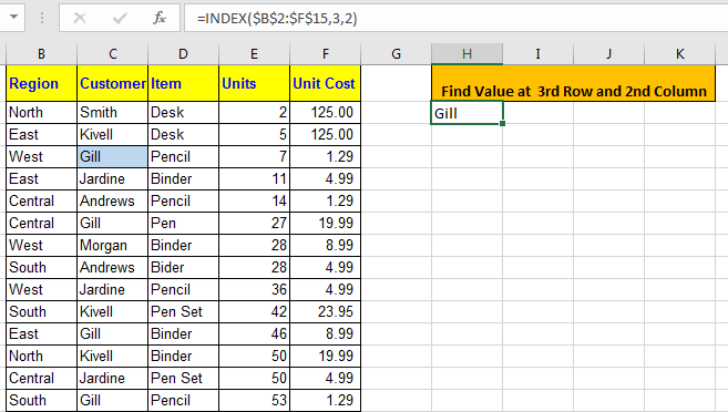
All of these might be confusing to understand. Let’s understand how to use the function using an example. Here we have this data.
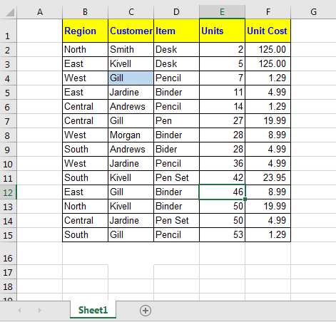
I want to retrieve data at the intersection of 3rd Row and 2nd Column. I write this INDEX formula in cell H2:
The result is Gill:
Reference Form INDEX Function
It is much like a multidimensional array index function. Actually in this form of INDEX function, we can give multiple arrays and then in the end we can tell the index from which array to pull data.
Excel INDEX Function Reference Form Syntax
=INDEX( (array1, array2,…), row number, [optional column number], [optional array number] )
(array1, array2,…) : This parenthesis contains a list of arrays. For example (A1:A10,D1:R100,…).
Row number : Ther row number in your array from which you want to get your value.
[optional column number] : This column number in array. It is optional. If omitted, the INDEX formula automatically takes 1 for it.
[optional array number] : The area number from which you want to pull data. In excel it is shown as area_num
Come, let’s have an example.
I have these 3 tables in Excel Worksheet.
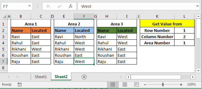
Area 1, Area 2 and Area 3 are my ranges as shown in the above image. I need to retrieve data according to values in cell L2, L3 and L4. So, I write this INDEX formula in cell M1.
=INDEX(($B$3:$C$7,$E$3:$F$7,$H$3:$I$7),L2,L3,L4)
Here L2 is 1, L3 is 2 and L4 is 1. Hence the INDEX function will return the value from the 1st row of the second column from the 1st array. And that is East.
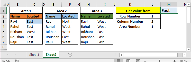
Now change L2 to 2 and L4 to 2. You will have West in M2, as shown in below image.
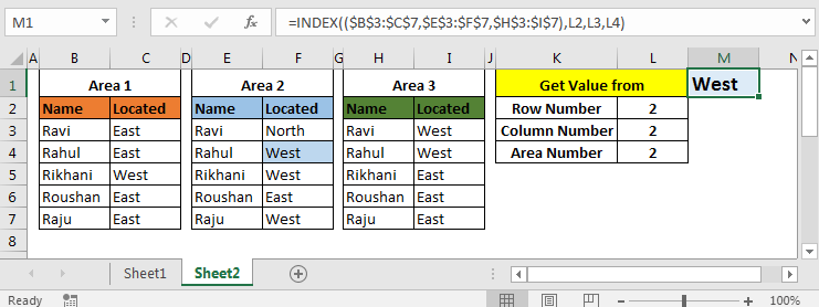
And so on.
The INDEX function in Excel is mostly used with MATCH Function. The INDEX MATCH function is so famous that it is sometimes thought of as one single function. Here I have explained the INDEX MATCH function with multiple criteria in detail. Go check it out. How to lookup values using the INDEX and MATCH function
Hope this article about How to use the INDEX function in Excel is explanatory. Find more articles on calculating values and related Excel formulas here. If you liked our blogs, share it with your friends on Facebook. And also you can follow us on Twitter and Facebook. We would love to hear from you, do let us know how we can improve, complement or innovate our work and make it better for you. Write to us at info@exceltip.com.
Related Articles :
Use INDEX and MATCH to Lookup Value : The INDEX & MATCH formula is used to lookup dynamically and precisely a value in a given table. This is an alternative to the VLOOKUP function and it overcomes the shortcomings of the VLOOKUP function.
Use VLOOKUP from Two or More Lookup Tables : To lookup from multiple tables we can take an IFERROR approach. To lookup from multiple tables, it takes the error as a switch for the next table. Another method can be an If approach.
How to do Case Sensitive Lookup in Excel : The excel’s VLOOKUP function isn’t case sensitive and it will return the first matched value from the list. INDEX-MATCH is no exception but it can be modified to make it case sensitive.
Lookup Frequently Appearing Text with Criteria in Excel : The lookup most frequently appears in text in a range we use the INDEX-MATCH with MODE function.
Popular Articles :
How to use the IF Function in Excel : The IF statement in Excel checks the condition and returns a specific value if the condition is TRUE or returns another specific value if FALSE.
How to use the VLOOKUP Function in Excel : This is one of the most used and popular functions of excel that is used to lookup value from different ranges and sheets.
How to use the SUMIF Function in Excel : This is another dashboard essential function. This helps you sum up values on specific conditions.
How to use the COUNTIF Function in Excel : Count values with conditions using this amazing function. You don’t need to filter your data to count specific values. Countif function is essential to prepare your dashboard.
Содержание
- Использование функции ИНДЕКС
- Способ 1: использование оператора ИНДЕКС для массивов
- Способ 2: применение в комплексе с оператором ПОИСКПОЗ
- Способ 3: обработка нескольких таблиц
- Способ 4: вычисление суммы
- Вопросы и ответы

Одной из самых полезных функций программы Эксель является оператор ИНДЕКС. Он производит поиск данных в диапазоне на пересечении указанных строки и столбца, возвращая результат в заранее обозначенную ячейку. Но полностью возможности этой функции раскрываются при использовании её в сложных формулах в комбинации с другими операторами. Давайте рассмотрим различные варианты её применения.
Использование функции ИНДЕКС
Оператор ИНДЕКС относится к группе функций из категории «Ссылки и массивы». Он имеет две разновидности: для массивов и для ссылок.
Вариант для массивов имеет следующий синтаксис:
=ИНДЕКС(массив;номер_строки;номер_столбца)
При этом два последних аргумента в формуле можно использовать, как вместе, так и любой один из них, если массив одномерный. При многомерном диапазоне следует применять оба значения. Нужно также учесть, что под номером строки и столбца понимается не номер на координатах листа, а порядок внутри самого указанного массива.
Синтаксис для ссылочного варианта выглядит так:
=ИНДЕКС(ссылка;номер_строки;номер_столбца;[номер_области])
Тут точно так же можно использовать только один аргумент из двух: «Номер строки» или «Номер столбца». Аргумент «Номер области» вообще является необязательным и он применяется только тогда, когда в операции участвуют несколько диапазонов.
Таким образом, оператор ищет данные в установленном диапазоне при указании строки или столбца. Данная функция своими возможностями очень похожа на оператора ВПР, но в отличие от него может производить поиск практически везде, а не только в крайнем левом столбце таблицы.
Способ 1: использование оператора ИНДЕКС для массивов
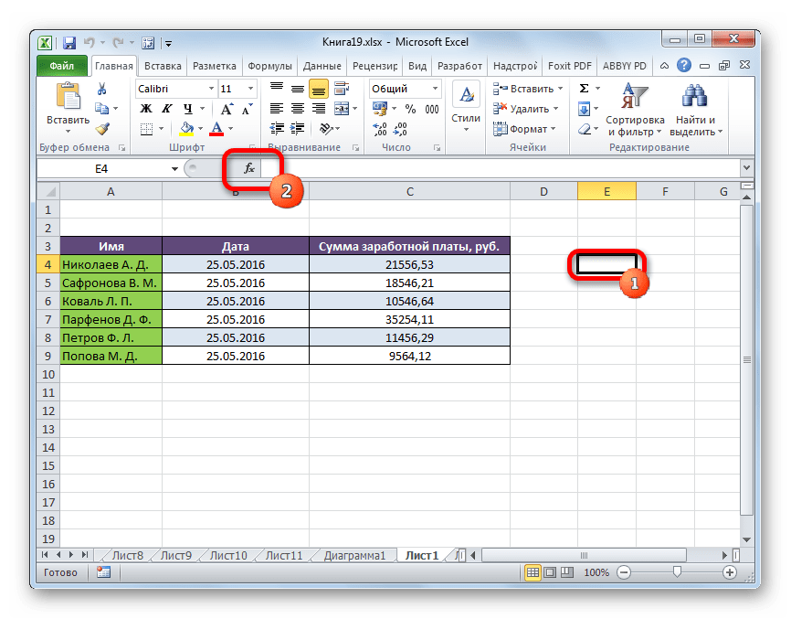
Давайте, прежде всего, разберем на простейшем примере алгоритм использования оператора ИНДЕКС для массивов.
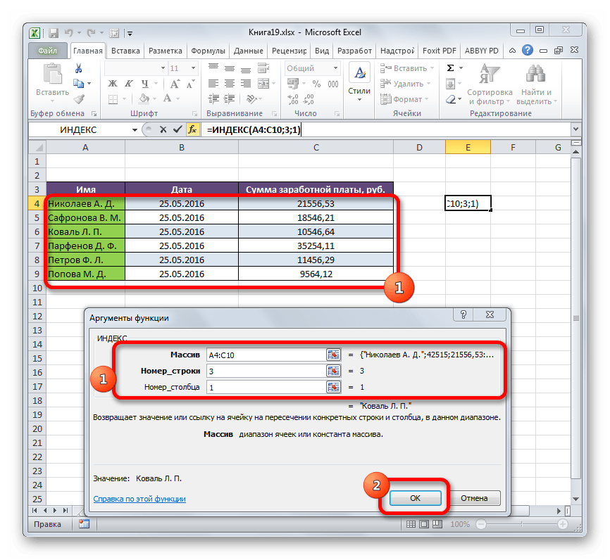
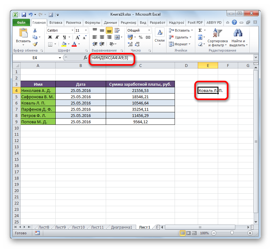
Имеем таблицу зарплат. В первом её столбце отображены фамилии работников, во втором – дата выплаты, а в третьем – величина суммы заработка. Нам нужно вывести имя работника в третьей строке.
- Выделяем ячейку, в которой будет выводиться результат обработки. Кликаем по значку «Вставить функцию», который размещен сразу слева от строки формул.
- Происходит процедура активации Мастера функций. В категории «Ссылки и массивы» данного инструмента или «Полный алфавитный перечень» ищем наименование «ИНДЕКС». После того, как нашли этого оператора, выделяем его и щелкаем по кнопке «OK», которая размещается в нижней части окна.
- Открывается небольшое окошко, в котором нужно выбрать один из типов функции: «Массив» или «Ссылка». Нужный нам вариант «Массив». Он расположен первым и по умолчанию выделен. Поэтому нам остается просто нажать на кнопку «OK».
- Открывается окно аргументов функции ИНДЕКС. Как выше говорилось, у неё имеется три аргумента, а соответственно и три поля для заполнения.
В поле «Массив» нужно указать адрес обрабатываемого диапазона данных. Его можно вбить вручную. Но для облегчения задачи мы поступим иначе. Ставим курсор в соответствующее поле, а затем обводим весь диапазон табличных данных на листе. После этого адрес диапазона тут же отобразится в поле.
В поле «Номер строки» ставим цифру «3», так как по условию нам нужно определить третье имя в списке. В поле «Номер столбца» устанавливаем число «1», так как колонка с именами является первой в выделенном диапазоне.
После того, как все указанные настройки совершены, щелкаем по кнопке «OK».
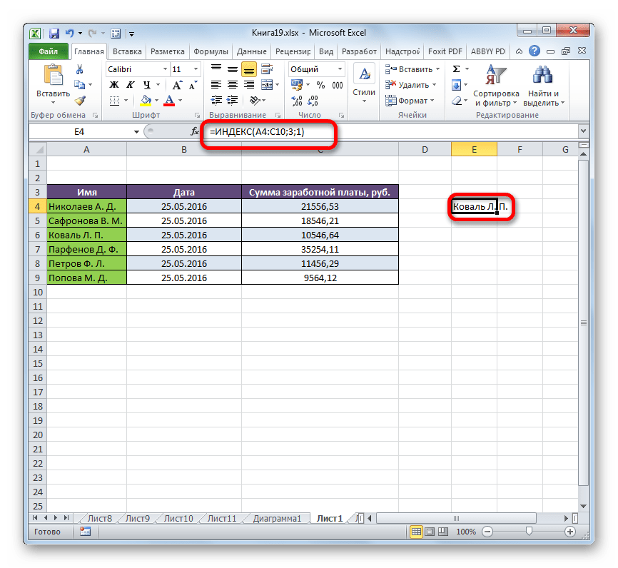
- Результат обработки выводится в ячейку, которая была указана в первом пункте данной инструкции. Именно выведенная фамилия является третьей в списке в выделенном диапазоне данных.


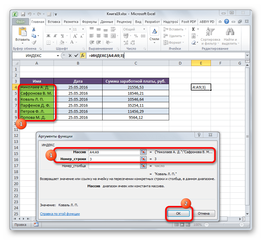
Мы разобрали применение функции ИНДЕКС в многомерном массиве (несколько столбцов и строк). Если бы диапазон был одномерным, то заполнение данных в окне аргументов было бы ещё проще. В поле «Массив» тем же методом, что и выше, мы указываем его адрес. В данном случае диапазон данных состоит только из значений в одной колонке «Имя». В поле «Номер строки» указываем значение «3», так как нужно узнать данные из третьей строки. Поле «Номер столбца» вообще можно оставить пустым, так как у нас одномерный диапазон, в котором используется только один столбец. Жмем на кнопку «OK».
Результат будет точно такой же, что и выше.
Это был простейший пример, чтобы вы увидели, как работает данная функция, но на практике подобный вариант её использования применяется все-таки редко.
Урок: Мастер функций в Экселе
Способ 2: применение в комплексе с оператором ПОИСКПОЗ
На практике функция ИНДЕКС чаще всего применяется вместе с аргументом ПОИСКПОЗ. Связка ИНДЕКС – ПОИСКПОЗ является мощнейшим инструментом при работе в Эксель, который по своему функционалу более гибок, чем его ближайший аналог – оператор ВПР.
Основной задачей функции ПОИСКПОЗ является указание номера по порядку определенного значения в выделенном диапазоне.
Синтаксис оператора ПОИСКПОЗ такой:
=ПОИСКПОЗ(искомое_значение, просматриваемый_массив, [тип_сопоставления])
- Искомое значение – это значение, позицию которого в диапазоне мы ищем;
- Просматриваемый массив – это диапазон, в котором находится это значение;
- Тип сопоставления – это необязательный параметр, который определяет, точно или приблизительно искать значения. Мы будем искать точные значения, поэтому данный аргумент не используется.
С помощью этого инструмента можно автоматизировать введение аргументов «Номер строки» и «Номер столбца» в функцию ИНДЕКС.
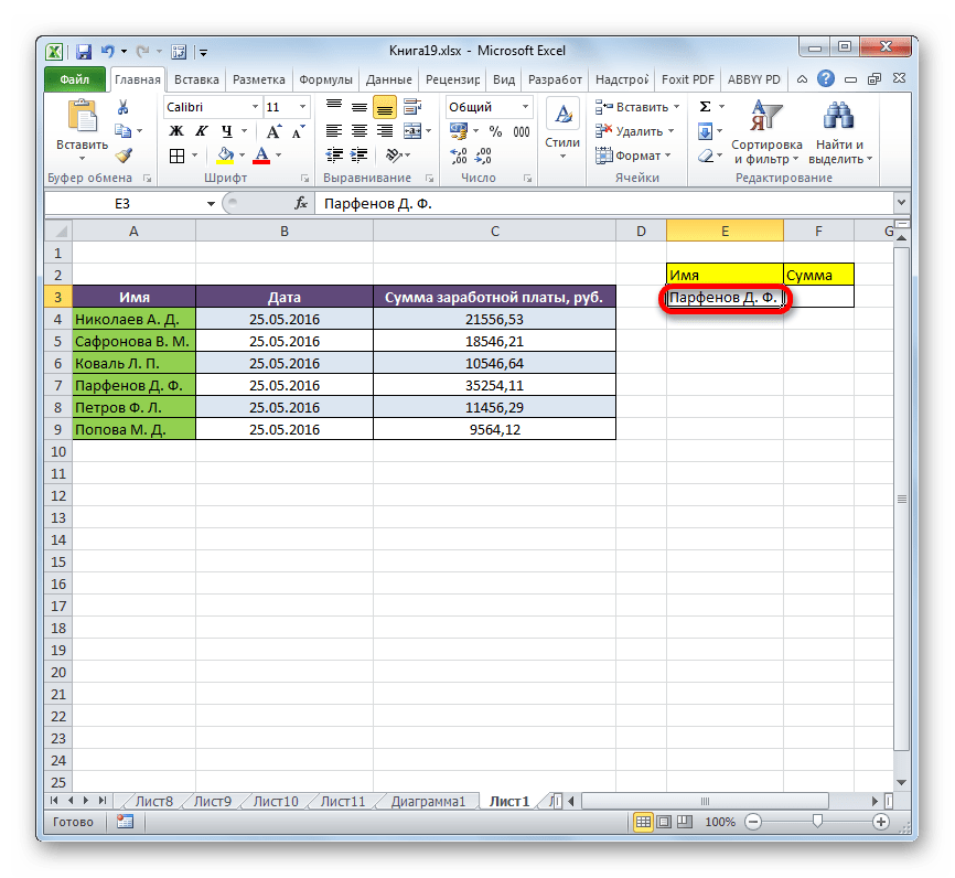
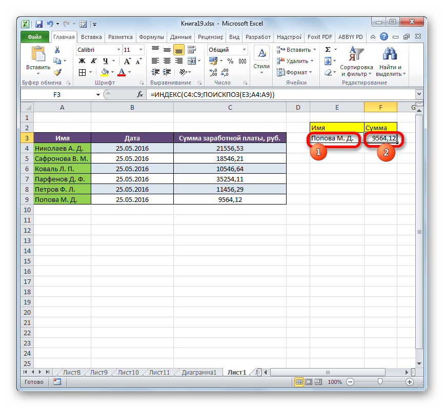
Посмотрим, как это можно сделать на конкретном примере. Работаем все с той же таблицей, о которой шла речь выше. Отдельно у нас имеется два дополнительных поля – «Имя» и «Сумма». Нужно сделать так, что при введении имени работника автоматически отображалась сумма заработанных им денег. Посмотрим, как это можно воплотить на практике, применив функции ИНДЕКС и ПОИСКПОЗ.
- Прежде всего, узнаем, какую заработную плату получает работник Парфенов Д. Ф. Вписываем его имя в соответствующее поле.
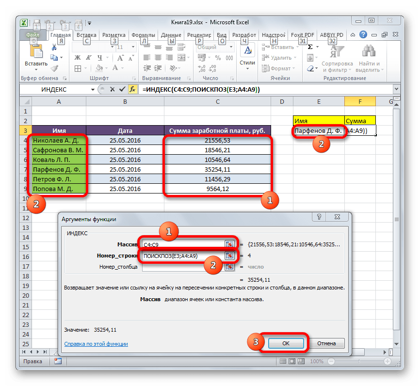
- Выделяем ячейку в поле «Сумма», в которой будет выводиться итоговый результат. Запускаем окно аргументов функции ИНДЕКС для массивов.
В поле «Массив» вносим координаты столбца, в котором находятся суммы заработных плат работников.
Поле «Номер столбца» оставляем пустым, так как мы используем для примера одномерный диапазон.
А вот в поле «Номер строки» нам как раз нужно будет записать функцию ПОИСКПОЗ. Для её записи придерживаемся того синтаксиса, о котором шла речь выше. Сразу в поле вписываем наименование самого оператора «ПОИСКПОЗ» без кавычек. Затем сразу же открываем скобку и указываем координаты искомого значения. Это координаты той ячейки, в которую мы отдельно записали фамилию работника Парфенова. Ставим точку с запятой и указываем координаты просматриваемого диапазона. В нашем случае это адрес столбца с именами сотрудников. После этого закрываем скобку.
После того, как все значения внесены, жмем на кнопку «OK».
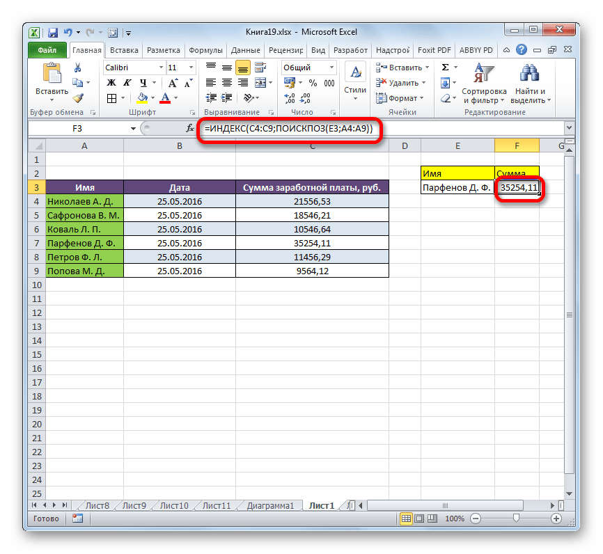
- Результат количества заработка Парфенова Д. Ф. после обработки выводится в поле «Сумма».
- Теперь, если в поле «Имя» мы изменим содержимое с «Парфенов Д.Ф.», на, например, «Попова М. Д.», то автоматически изменится и значение заработной платы в поле «Сумма».
Способ 3: обработка нескольких таблиц
Теперь посмотрим, как с помощью оператора ИНДЕКС можно обработать несколько таблиц. Для этих целей будет применяться дополнительный аргумент «Номер области».
Имеем три таблицы. В каждой таблице отображена заработная плата работников за отдельный месяц. Нашей задачей является узнать заработную плату (третий столбец) второго работника (вторая строка) за третий месяц (третья область).
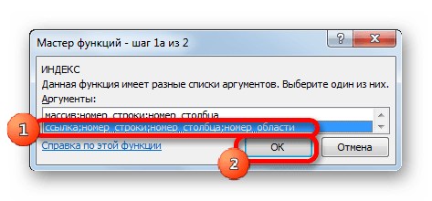
- Выделяем ячейку, в которой будет производиться вывод результата и обычным способом открываем Мастер функций, но при выборе типа оператора выбираем ссылочный вид. Это нам нужно потому, что именно этот тип поддерживает работу с аргументом «Номер области».
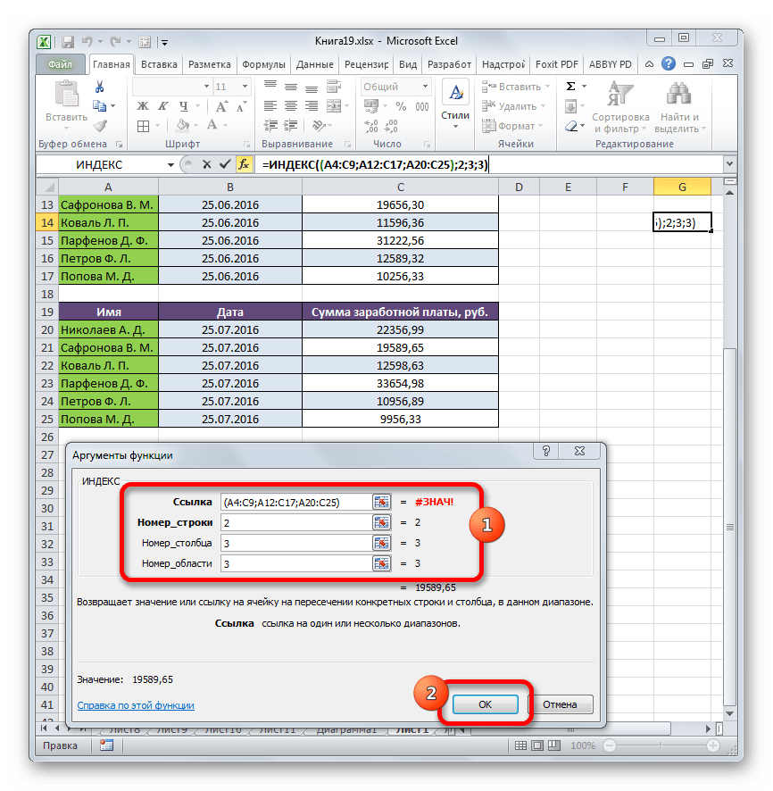
- Открывается окно аргументов. В поле «Ссылка» нам нужно указать адреса всех трех диапазонов. Для этого устанавливаем курсор в поле и выделяем первый диапазон с зажатой левой кнопкой мыши. Затем ставим точку с запятой. Это очень важно, так как если вы сразу перейдете к выделению следующего массива, то его адрес просто заменит координаты предыдущего. Итак, после введения точки с запятой выделяем следующий диапазон. Затем опять ставим точку с запятой и выделяем последний массив. Все выражение, которое находится в поле «Ссылка» берем в скобки.
В поле «Номер строки» указываем цифру «2», так как ищем вторую фамилию в списке.
В поле «Номер столбца» указываем цифру «3», так как колонка с зарплатой является третьей по счету в каждой таблице.
В поле «Номер области» ставим цифру «3», так как нам нужно найти данные в третьей таблице, в которой содержится информация о заработной плате за третий месяц.
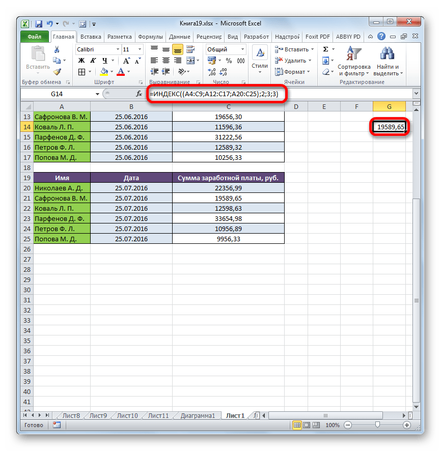
После того, как все данные введены, щелкаем по кнопке «OK».
- После этого в предварительно выделенную ячейку выводятся результаты вычисления. Там отображается сумма заработной платы второго по счету работника (Сафронова В. М.) за третий месяц.
Способ 4: вычисление суммы
Ссылочная форма не так часто применяется, как форма массива, но её можно использовать не только при работе с несколькими диапазонами, но и для других нужд. Например, её можно применять для расчета суммы в комбинации с оператором СУММ.
При сложении суммы СУММ имеет следующий синтаксис:
=СУММ(адрес_массива)
В нашем конкретном случае сумму заработка всех работников за месяц можно вычислить при помощи следующей формулы:
=СУММ(C4:C9)
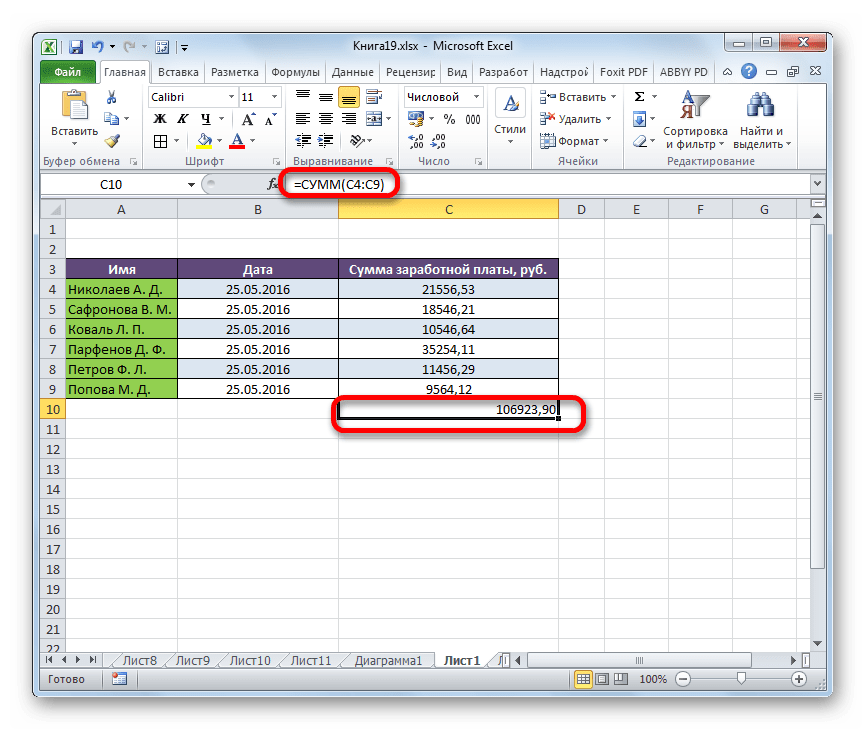
Но можно её немного модифицировать, использовав функцию ИНДЕКС. Тогда она будет иметь следующий вид:
=СУММ(C4:ИНДЕКС(C4:C9;6))
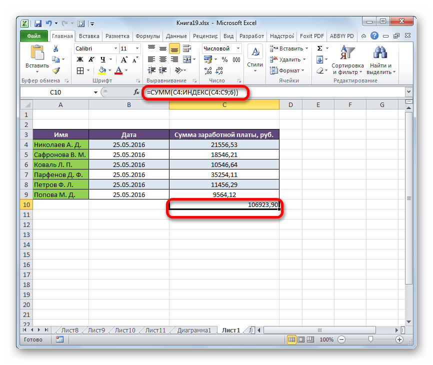
В этом случае в координатах начала массива указывается ячейка, с которой он начинается. А вот в координатах указания окончания массива используется оператор ИНДЕКС. В данном случае первый аргумент оператора ИНДЕКС указывает на диапазон, а второй – на последнюю его ячейку – шестую.
Урок: Полезные функции Excel
Как видим, функцию ИНДЕКС можно использовать в Экселе для решения довольно разноплановых задач. Хотя мы рассмотрели далеко не все возможные варианты её применения, а только самые востребованные. Существует два типа этой функции: ссылочный и для массивов. Наиболее эффективно её можно применять в комбинации с другими операторами. Созданные таким способом формулы смогут решать самые сложные задачи.
What is the INDEX Function in Excel?
The INDEX function in Excel provides the value of a cell within a selected range against a given row and column. For example, the formula = INDEX(“Employee ID”,row_num,[column_num]) will return the Employee ID 27 against the given row number 5 and column number 3.
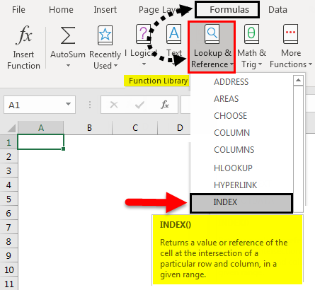
Using the INDEX function, we can find the value at the intersection of a specific row and column. The INDEX function in Excel is present under the Microsoft Excel Lookup and Reference function.
Key Highlights
- The INDEX function in Excel helps to find the information within a data range, where it looks up values by both columns and rows.
- It looks up the value of a cell at the intersection of a given row and column.
- We use the INDEX function in Excel with the MATCH function more commonly. The combination of the INDEX and MATCH functions is an alternative to the VLOOKUP function, which is more powerful & flexible.
- We can use the INDEX function in Excel to fetch individual values or entire rows and columns.
INDEX Function in Excel Syntax
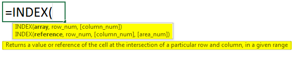
There are two types of the INDEX function in Excel:
#1 Array Form
We use the Array INDEX form when the cell we refer to is within a single range of the data table, e.g., A3:C7.
To understand better, refer to the below image-
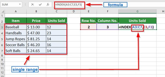
Syntax-
= INDEX (array, row_num, [column_num])
#2 Reference Form
We use this INDEX form when the cell that we are referring to is within multiple cell ranges, e.g., (A7:C1,A12:C14,A16:C19)
Refer to the below image-
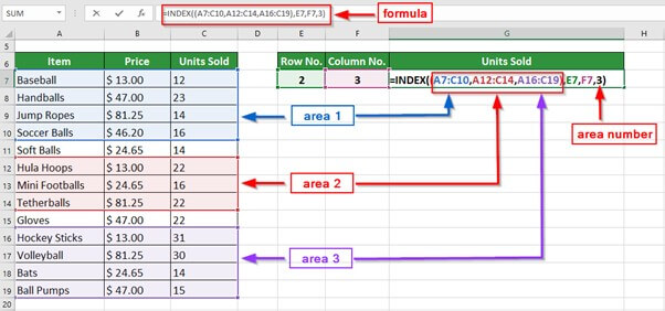
Syntax-
=INDEX (reference,row_num,[col_num],[area_num])
Explanation of the Syntax
array:
It is a compulsory or required argument that indicates the range or array of cells we want to look up
Note: If there are multiple cell ranges in the data table, it is called a reference where all the cell ranges(areas) are separated by a comma and with closed brackets
row_num:
It is a compulsory or required argument that indicates the row number against which we want to fetch the value.
Note: Excel considers the row_num argument optional if only one row exists in an array or cell range.
col_num:
It is a compulsory or required argument that indicates the column number against which we want to fetch the value.
Note: Excel considers the col_num argument optional if only one column exists in an array or cell range.
area_num:
It is an optional argument. If the desired value is present in multiple cell ranges in the data table, the area_num indicates the cell range to use.
Note: If there is no value in area_num, then by default, the INDEX Function in Excel considers the first area as the area number.
How to Use the INDEX Function in Excel?
To understand the usage of the INDEX function, consider the below-given examples.
You can download this INDEX Function in Excel Template here – INDEX Function in Excel Template
ARRAY FORM
Example #1:
The table contains the name of Employees of a company, their Employee ID, Gender, and Age. We want to find the Employee ID of Methos using the INDEX function.
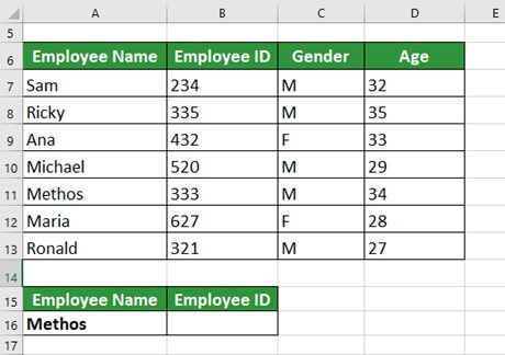
Solution:
We will apply the INDEX formula in cell B16 to get the Employee ID of Methos.
Step 1: Click on the Insert Function (fx) option under the Formulas section of the Excel toolbar.
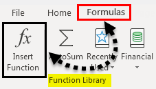
An Insert Function dialog box appears.
Step 2: Type INDEX in the dialog box’s Search for a function option. And double click the INDEX option from the list.
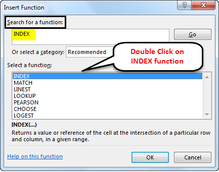
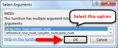
A Select Arguments dialog box shows the two types of INDEX functions: one for array and the other for reference.
Step 3: Select the array formula, as we have only one data range, and click OK.
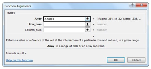
A Function Arguments dialog box opens with options Array, row_num, and column_num.
Step 4: Enter the cell range (A7:D13) that contains the lookup value in the Array argument
Note: Do not select the column headings
Step 5: Enter the row number(5) that contains the lookup value in the row_num argument.
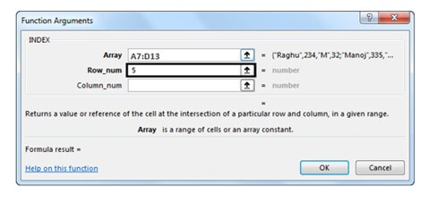
Step 6: Enter the column number(2) that contains the lookup value in the Col_num argument.
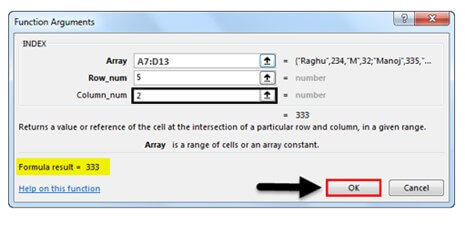
Step 7: Click OK to get the below result
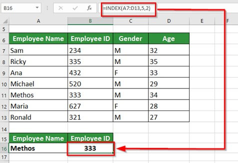
The Index function will return the value of the 5th row and 2nd column, i.e., Employee ID 333.
Example #2
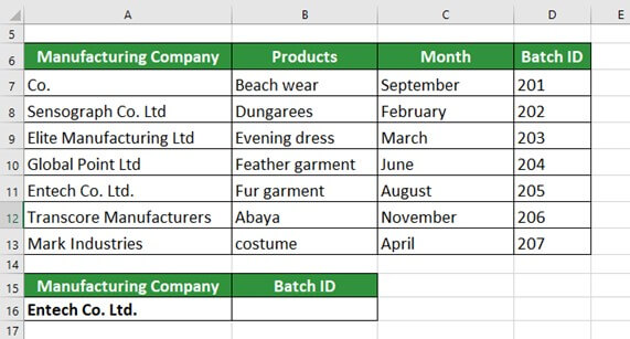
The table below shows the Batch ID of Clothing products manufactured by different industries. We want to find the Batch ID of products manufactured by Entech Co. Ltd.
Solution:
Step 1: Write Entech Co. Ltd. in cell A16
Step 2: Place the cursor in cell B16 and enter the formula,
=INDEX(A7:D13,5,4)
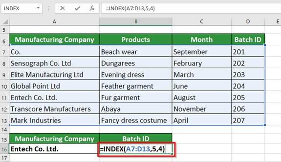
Explanation:
A7:D13: It is the cell range that contains data about Entech Co. Ltd.
5,4: The lookup value- Entech Co. Ltd. is in the 5th row of the selected cell range with Batch ID in the 4th column.
Therefore, we write 5 & 4, respectively, in the formula.
Step 3: Press the Enter key to get the below result
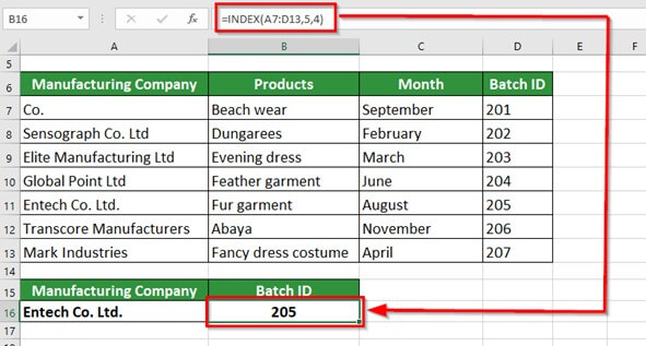
The INDEX function with Array Form gives the Batch ID of 205 for products manufactured by Entech Co. Ltd.
Example #3
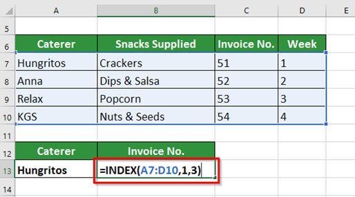
The table below shows 4 different caterers with snacks they supplied and invoice numbers for their respective bills. Here, we want to find the invoice number for the bill of the snacks supplied by Hungritos.
Solution:
Step 1: Write Hungritos in cell A13
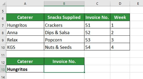
Step 2: Place the cursor in cell B13 and enter the formula,
=INDEX(A7:D10,1,3)
Explanation:
A7:D10- It is the cell range that contains the data of Hingritos.
Note: We do not select the headings of the table.
1,3- The lookup value- Hingritos is in the 1st row of the selected range with invoice no. in the 3rd column. Therefore, we write 1 & 3, respectively, in the formula.
Step 3: Press the Enter key to get the below result
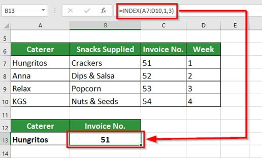
The INDEX function returns invoice no. 51 for snacks provided by Hungritos.
REFERENCE FORM
Example #1
The table below shows three different tables with Employee Name, Employee ID, Gender, Age, and Department. We want to find the Employee ID of Maria using the INDEX function in Excel.
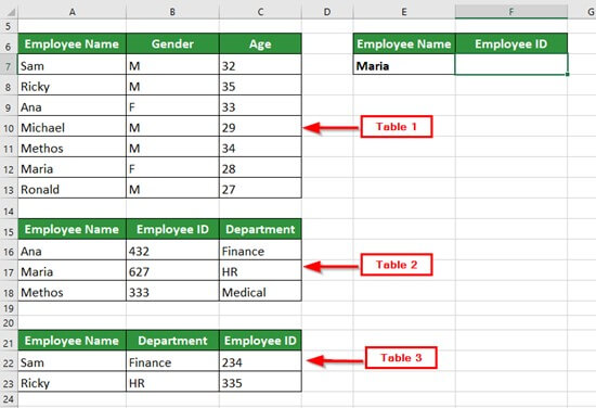
Solution:
Here, we will use the Reference Form of Excel since there are three different data tables.
Step 1: Write Maria in cell E7
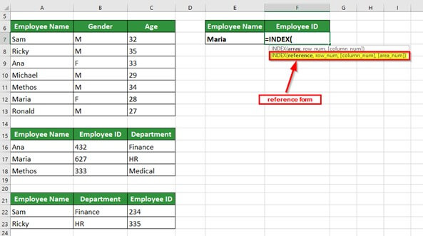
Step 2: Place the cursor in cell F7 and type =INDEX(
When we type the above, it displays two arguments, as shown in the image below
Step 3: Enter the formula,
=INDEX((A7:C13,A16:C18,A22:C23),2,2,2)
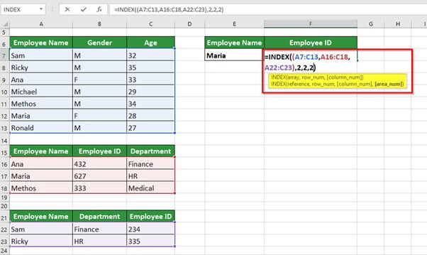
- Row_num: It is the row against which we want to fetch the Employee ID of Maria present in table 2; therefore, we enter row number(2), the intersection will occur at the 2nd row of the table
- Col_num: It is the column against which we want to fetch the value, i.e., 2, the intersection will occur at the 2nd column of the 2nd table
- Area_num: It indicates the area(table) which contains the details of Maria, i.e., table 2. Thus, we enter the Area_num as number 2 here.
Step 4: Press the Enter key to get the below output
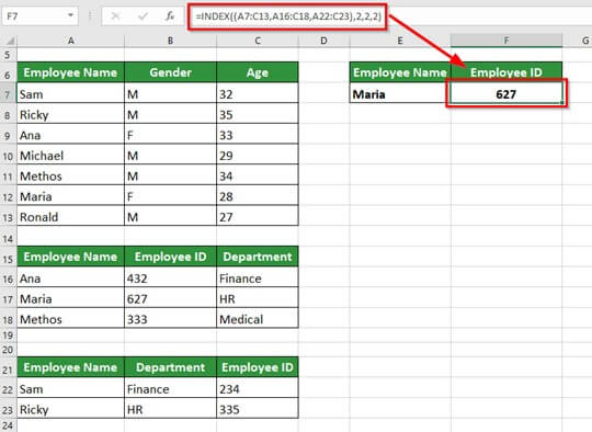
The INDEX function in Excel returns Employee ID of Maria as 627.
Example #2
The table below shows sports items sold by a store with their prices. We want to find the number of Volleyballs sold by the store given the row number and column number.
Solution:
Step 1: Write the desired row and column numbers in cells E7 and F7, respectively.
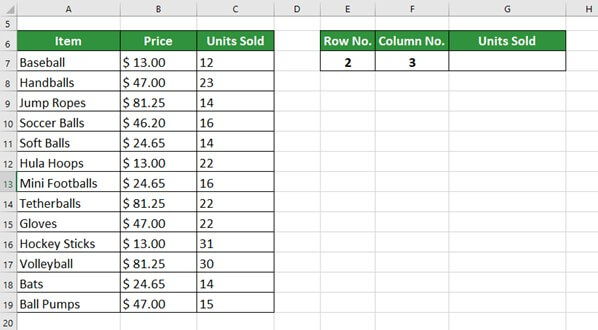
Step 2: Place the cursor in cell G7 and enter the formula,
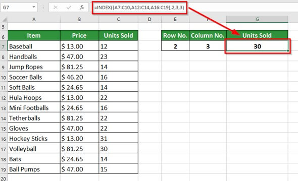
=INDEX((A7:C10,A12:C14,A16:C19),2,3,3)
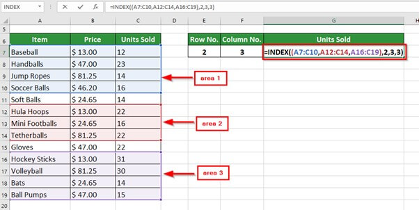
The table above has three different areas- area 1, area 2, and area 3. Our desired item, a Volleyball, is in the third area. Therefore, we write the number 3 at the end.
Step 3: Press the Enter key to give the below result.
Things to Remember
- The INDEX function in Excel returns #VALUE! Error if row_num/ column_num is not mentioned in the formula or given as 0.
- The INDEX function returns #VALUE! error if the values for row_num, col_num, or area_num are non-numeric.
- The INDEX function in Excel returns #REF! Error if the value entered for row_num exceeds the number of rows present in the data table
- The INDEX function returns #REF! Error if the value entered for column_num exceeds the number of columns present in the data table
- The INDEX function in Excel returns #REF! Error if we provide a value for area_num greater than the number of areas in the cell range.
- If we give (refer) the area_num in the INDEX Formula from another sheet, the Index Function in Excel returns #VALUE! Error. It should represent the table present in the same sheet.
Frequently Asked Questions (FAQs)
Q1) What is the use of INDEX ()?
Answer: With the INDEX (), we can find the index position of an element or character in an item string. It gives the lowest possible index of the specified element in the list. If the provided item is not in the list, the INDEX function in Excel returns a ValueError.
Q2) What is the INDEX formula?
Answer: The INDEX formula for the Array form is
=INDEX(array, row_num, [col_num]).
The INDEX formula for Reference form is =INDEX(reference,row_num,[column_num],[area_num]).
The array argument specifies the cell range we want to look up. If there are multiple cell ranges in the data table, we separate them using a comma and close them with brackets; row_num indicates the row number against which we want to fetch the value; col_num indicates the column number against which we want to fetch the value; area_num indicates the range to use if there are multiple areas(tables).
Q3) What is the purpose of the INDEX and MATCH functions?
The INDEX function provides the value of a parameter based on the row and column numbers. The MATCH function gives the position of a cell in a column or a row. Combining the INDEX and MATCH functions provides a cell value based on horizontal and vertical criteria.
Recommended Articles
The article is a guide to the INDEX Function in Excel. Here we discuss how to use the INDEX Function in Excel, with practical examples and a downloadable excel template. Enhance your knowledge with these useful functions in excel
- Excel INDEX Function
- INDEX MATCH Function in Excel
- Time Function in Excel
- VBA Color Index