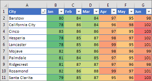
How to do excel conditional formatting - Word и Excel - помощь в работе с программами

Conditional formatting can help make patterns and trends in your data more apparent. To use it, you create rules that determine the format of cells based on their values, such as the following monthly temperature data with cell colors tied to cell values.

You can apply conditional formatting to a range of cells (either a selection or a named range), an Excel table, and in Excel for Windows, even a PivotTable report.

Conditional formatting typically works the same way in a range of cells, an Excel table, or a PivotTable report. However, conditional formatting in a PivotTable report has some extra considerations:

There are some conditional formats that don’t work with fields in the Values area of a PivotTable report. For example, you can’t format such fields based on whether they contain unique or duplicate values. These restrictions are mentioned in the remaining sections of this article, where applicable.
If you change the layout of the PivotTable report by filtering, hiding levels, collapsing and expanding levels, or moving a field, the conditional format is maintained as long as the fields in the underlying data are not removed.
The scope of the conditional format for fields in the Values area can be based on the data hierarchy and is determined by all the visible children (the next lower level in a hierarchy) of a parent (the next higher level in a hierarchy) on rows for one or more columns, or columns for one or more rows.

Note: In the data hierarchy, children do not inherit conditional formatting from the parent, and the parent does not inherit conditional formatting from the children.
There are three methods for scoping the conditional format of fields in the Values area: by selection, by corresponding field, and by value field.

The default method of scoping fields in the Values area is by selection. You can change the scoping method to the corresponding field or value field by using the Apply formatting rule to option button, the New Formatting Rule dialog box, or the Edit Formatting Rule dialog box.

Method	Use this method if you want to select
Scoping by selection	A contiguous set of fields in the Values area, such as all of the product totals for one region. A non-contiguous set of fields in the Values area, such as product totals for different regions across levels in the data hierarchy.
Scoping by value field	Avoid making many non-contiguous selections. Conditionally format a set of fields in the Values area for all levels in the hierarchy of data. Include subtotals and grand totals.
Scoping by corresponding field	Avoid making many non-contiguous selections. Conditionally format a set of fields in the Values area for one level in the hierarchy of data. Exclude subtotals. When you conditionally format fields in the Values area for top, bottom, above average, or below average values, the rule is based on all visible values by default. However, when you scope by corresponding field, instead of using all visible values, you can apply the conditional format for each combination of: A column and its parent row field. A row and its parent column field.

Note: Quick Analysis is not available in Excel 2010 and previous versions.

Use the Quick Analysis button to apply selected conditional formatting to the selected data. The Quick Analysis button appears automatically when you select data.

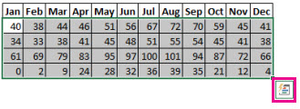
Select the data that you want to conditionally format. The Quick Analysis button appears on the lower-right corner of the selection.
Click the Quick Analysis button , or press Ctrl+Q.
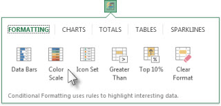
In the pop-up that appears, on the Formatting tab, move your mouse over the different options to see a Live Preview on your data, and then click on the formatting option you want.
Notes:
- The formatting options that appear in the Formatting tab depend on the data you have selected. If your selection contains only text, then the available options are Text, Duplicate, Unique, Equal To, and Clear. When the selection contains only numbers, or both text and numbers, then the options are Data Bars, Colors, Icon Sets, Greater, Top 10%, and Clear.
- Live preview will only render for those formatting options that can be used on your data. For example, if your selected cells don’t contain matching data and you select Duplicate, the live preview will not work.
If the Text that Contains dialog box appears, enter the formatting option you want to apply and click OK.

If you’d like to watch a video that shows how to use Quick Analysis to apply conditional formatting, see Video: Use conditional formatting.

You can download a sample workbook that contains different examples of applying conditional formatting, both with standard rules such as top and bottom, duplicates, Data Bars, Icon Sets and Color Scales, as well as manually creating rules of your own.

Download: Conditional formatting examples in Excel

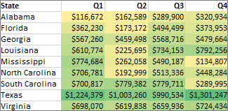
Color scales are visual guides that help you understand data distribution and variation. A two-color scale helps you compare a range of cells by using a gradation of two colors. The shade of the color represents higher or lower values. For example, in a green and yellow color scale, as shown below, you can specify that higher value cells have a more green color and lower value cells have a more yellow color.

Tip: You can sort cells that have this format by their color — just use the context menu.

Tip: If any cells in the selection contain a formula that returns an error, the conditional formatting is not applied to those cells. To ensure that the conditional formatting is applied to those cells, use an IS or IFERROR function to return a value other than an error value.

Quick formatting

Select one or more cells in a range, table, or PivotTable report.
On the Home tab, in the Styles group, click the arrow next to Conditional Formatting, and then click Color Scales.
Select a two-color scale.

Hover over the color scale icons to see which icon is a two-color scale. The top color represents higher values, and the bottom color represents lower values.

You can change the method of scoping for fields in the Values area of a PivotTable report by using the Formatting Options button that appears next to a PivotTable field that has conditional formatting applied.

Advanced formatting

Select one or more cells in a range, table, or PivotTable report.
On the Home tab, in the Styles group, click the arrow next to Conditional Formatting, and then click Manage Rules. The Conditional Formatting Rules Manager dialog box appears.
Do one of the following:
- To add a completely new conditional format, click New Rule. The New Formatting Rule dialog box appears.
- To add a new conditional format based on one that is already listed, select the rule, then click Duplicate Rule. The duplicate rule appears in the dialog box. Select the duplicate, then select Edit Rule. The Edit Formatting Rule dialog box appears.
- To change a conditional format, do the following:
  1. Make sure that the appropriate worksheet, table, or PivotTable report is selected in the Show formatting rules for list box.
  2. Optionally, change the range of cells by clicking Collapse Dialog in the Applies to box to temporarily hide the dialog box, by selecting the new range of cells on the worksheet, and then by selecting Expand Dialog.
  3. Select the rule, and then click Edit rule. The Edit Formatting Rule dialog box appears.
Under Apply Rule To, to optionally change the scope for fields in the Values area of a PivotTable report by:
- Selection: Click Selected cells.
- All cells for a Value label: Click All cells showing <Value label> values.
- All cells for a Value label, excluding subtotals and the grand total: Click All cells showing <Value label> values for <Row Label>.
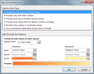
Under Select a Rule Type, click Format all cells based on their values (default).
Under Edit the Rule Description, in the Format Style list box, select 2-Color Scale.
To select a type in the Type box for Minimum and Maximum, do one of the following:
- Format lowest and highest values: Select Lowest Value and Highest Value.
  
  In this case, you do not enter a Minimum and MaximumValue.
- Format a number, date, or time value: Select Number and then enter a Minimum and MaximumValue.
- Format a percentage Percent: Enter a Minimum and MaximumValue.
  
  Valid values are from 0 (zero) to 100. Don’t enter a percent sign.
  
  Use a percentage when you want to visualize all values proportionally because the distribution of values is proportional.
- Format a percentile: Select Percentile and then enter a Minimum and MaximumValue. Valid percentiles are from 0 (zero) to 100.
  
  Use a percentile when you want to visualize a group of high values (such as the top 20thpercentile) in one color grade proportion and low values (such as the bottom 20th percentile) in another color grade proportion, because they represent extreme values that might skew the visualization of your data.
- Format a formula result: Select Formula and then enter values for Minimum and Maximum.
  - The formula must return a number, date, or time value.
  - Start the formula with an equal sign (=).
  - Invalid formulas result in no formatting being applied.
  - It’s a good idea to test the formula to make sure that it doesn’t return an error value.
    Notes:
    - Make sure that the Minimum value is less than the Maximum value.
    - You can choose a different type for the Minimum and Maximum. For example, you can choose a number for Minimum a percentage for Maximum.
To choose a Minimum and Maximum color scale, click Color for each, and then select a color.

If you want to choose additional colors or create a custom color, click More Colors. The color scale you select is shown in the Preview box.

Color scales are visual guides that help you understand data distribution and variation. A three-color scale helps you compare a range of cells by using a gradation of three colors. The shade of the color represents higher, middle, or lower values. For example, in a green, yellow, and red color scale, you can specify that higher value cells have a green color, middle value cells have a yellow color, and lower value cells have a red color.

Tip: You can sort cells that have this format by their color — just use the context menu.

Quick formatting

Select one or more cells in a range, table, or PivotTable report.
On the Home tab, in the Styles group, click the arrow next to Conditional Formatting, and then click Color Scales.
Select a three-color scale. The top color represents higher values, the center color represents middle values, and the bottom color represents lower values.

Hover over the color scale icons to see which icon is a three-color scale.

Advanced formatting

Select one or more cells in a range, table, or PivotTable report.
On the Home tab, in the Styles group, click the arrow next to Conditional Formatting, and then click Manage Rules. The Conditional Formatting Rules Manager dialog box appears.
Do one of the following:
- To add a new conditional format, click New Rule. The New Formatting Rule dialog box appears.
- To add a new conditional format based on one that is already listed, select the rule, then click Duplicate Rule. The duplicate rule is copied and appears in the dialog box. Select the duplicate, then select Edit Rule. The Edit Formatting Rule dialog box appears.
- To change a conditional format, do the following:
  1. Make sure that the appropriate worksheet, table, or PivotTable report is selected in the Show formatting rules for list box.
  2. Optionally, change the range of cells by clicking Collapse Dialog in the Applies to box to temporarily hide the dialog box, by selecting the new range of cells on the worksheet, and then by selecting Expand Dialog.
  3. Select the rule, and then click Edit rule. The Edit Formatting Rule dialog box appears.
Under Apply Rule To, to optionally change the scope for fields in the Values area of a PivotTable report by:
- Selection: Click Just these cells.
- Corresponding field: Click All <value field> cells with the same fields.
- Value field: Click All <value field> cells.
Under Select a Rule Type, click Format all cells based on their values.
Under Edit the Rule Description, in the Format Style list box, select 3-Color Scale.
Select a type for Minimum, Midpoint, and Maximum. Do one of the following:
- Format lowest and highest values: Select a Midpoint.
  
  In this case, you do not enter a Lowest and HighestValue.
- Format a number, date, or time value: Select Number and then enter a value for Minimum, Midpoint, and Maximum.
- Format a percentage: Select Percent and then enter a value for Minimum, Midpoint, and Maximum. Valid values are from 0 (zero) to 100. Do not enter a percent (%) sign.
  
  Use a percentage when you want to visualize all values proportionally, because using a percentage ensures that the distribution of values is proportional.
- Format a percentile: Select Percentile and then enter a value for Minimum, Midpoint, and Maximum.
  
  Valid percentiles are from 0 (zero) to 100.
  
  Use a percentile when you want to visualize a group of high values (such as the top 20th percentile) in one color grade proportion and low values (such as the bottom 20th percentile) in another color grade proportion, because they represent extreme values that might skew the visualization of your data.
- Format a formula result: Select Formula and then enter a value for Minimum, Midpoint, and Maximum.
  
  The formula must return a number, date, or time value. Start the formula with an equal sign (=). Invalid formulas result in no formatting being applied. It’s a good idea to test the formula to make sure that it doesn’t return an error value.
  Notes:
  - You can set minimum, midpoint, and maximum values for the range of cells. Make sure that the value in Minimum is less than the value in Midpoint, which in turn is less than the value in Maximum.
  - You can choose a different type for Minimum, Midpoint, and Maximum. For example, you can choose a Minimum number, Midpoint percentile, and Maximum percent.
  - In many cases, the default Midpoint value of 50 percent works best, but you can adjust this to fit unique requirements.
To choose a Minimum, Midpoint, and Maximum color scale, click Color for each, and then select a color.
- To choose additional colors or create a custom color, click More Colors.
- The color scale you select is shown in the Preview box.

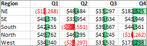
A data bar helps you see the value of a cell relative to other cells. The length of the data bar represents the value in the cell. A longer bar represents a higher value, and a shorter bar represents a lower value. Data bars are useful in spotting higher and lower numbers, especially with large amounts of data, such as top selling and bottom selling toys in a holiday sales report.

The example shown here uses data bars to highlight dramatic positive and negative values. You can format data bars so that the data bar starts in the middle of the cell, and stretches to the left for negative values.

Tip: If any cells in the range contain a formula that returns an error, the conditional formatting is not applied to those cells. To ensure that the conditional formatting is applied to those cells, use an IS or IFERROR function to return a value (such as 0 or «N/A») instead of an error value.

Quick formatting

Select one or more cells in a range, table, or PivotTable report.
On the Home tab, in the Style group, click the arrow next to Conditional Formatting, click Data Bars, and then select a data bar icon.

You can change the method of scoping for fields in the Values area of a PivotTable report by using the Apply formatting rule to option button.

Advanced formatting

Select one or more cells in a range, table, or PivotTable report.
On the Home tab, in the Styles group, click the arrow next to Conditional Formatting, and then click Manage Rules. The Conditional Formatting Rules Manager dialog box appears.
Do one of the following:
- To add a conditional format, click New Rule. The New Formatting Rule dialog box appears.
- To add a new conditional format based on one that is already listed, select the rule, then click Duplicate Rule. The duplicate rule is copied and appears in the dialog box. Select the duplicate, then select Edit Rule. The Edit Formatting Rule dialog box appears.
- To change a conditional format, do the following:
- 1. Make sure that the appropriate worksheet, table, or PivotTable report is selected in the Show formatting rules for list box.
  2. Optionally, change the range of cells by clicking Collapse Dialog in the Applies to box to temporarily hide the dialog box, by selecting the new range of cells on the worksheet, and then by selecting Expand Dialog.
  3. Select the rule, and then click Edit rule. The Edit Formatting Rule dialog box appears.
Under Apply Rule To, to optionally change the scope for fields in the Values area of a PivotTable report by:
- Selection: Click Just these cells.
- Corresponding field: Click All <value field> cells with the same fields.
- Value field: Click All <value field> cells.
Under Select a Rule Type, click Format all cells based on their values.
Under Edit the Rule Description, in the Format Style list box, select Data Bar.
Select a Minimum and MaximumType. Do one of the following:
- Format lowest and highest values: Select Lowest Value and Highest Value.
  
  In this case, you do not enter a value for Minimum and Maximum.
- Format a number, date, or time value: Select Number and then enter a Minimum and MaximumValue.
- Format a percentage: Select Percent and then enter a value for Minimum and Maximum.
  
  Valid values are from 0 (zero) to 100. Do not enter a percent (%) sign.
  
  Use a percentage when you want to visualize all values proportionally, because using a percentage ensures that the distribution of values is proportional.
- Format a percentile Select Percentile and then enter a value for Minimum and Maximum.
  
  Valid percentiles are from 0 (zero) to 100.
  
  Use a percentile when you want to visualize a group of high values (such as the top 20th percentile) in one data bar proportion and low values (such as the bottom 20th percentile) in another data bar proportion, because they represent extreme values that might skew the visualization of your data.
- Format a formula result Select Formula, and then enter a value for Minimum and Maximum.
  - The formula has to return a number, date, or time value.
  - Start the formula with an equal sign (=).
  - Invalid formulas result in no formatting being applied.
  - It’s a good idea to test the formula to make sure that it doesn’t return an error value.
Notes:
- Make sure that the Minimum value is less than the Maximum value.
- You can choose a different type for Minimum and Maximum. For example, you can choose a Minimum number and a Maximum percent.
To choose a Minimum and Maximum color scale, click Bar Color.

If you want to choose additional colors or create a custom color, click More Colors. The bar color you select is shown in the Preview box.
To show only the data bar and not the value in the cell, select Show Bar Only.
To apply a solid border to data bars, select Solid Border in the Border list box and choose a color for the border.
To choose between a solid bar and a gradiated bar, choose Solid Fill or Gradient Fill in the Fill list box.
To format negative bars, click Negative Value and Axis and then, in the Negative Value and Axis Settings dialog box, choose options for the negative bar fill and border colors. You can choose position settings and a color for the axis. When you are finished selecting options, click OK.
You can change the direction of bars by choosing a setting in the Bar Direction list box. This is set to Context by default, but you can choose between a left-to-right and a right-to-left direction, depending on how you want to present your data.

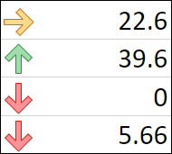
Use an icon set to annotate and classify data into three to five categories separated by a threshold value. Each icon represents a range of values. For example, in the 3 Arrows icon set, the green up arrow represents higher values, the yellow sideways arrow represents middle values, and the red down arrow represents lower values.

Tip: You can sort cells that have this format by their icon — just use the context menu.

The example shown here works with several examples of conditional formatting icon sets.

You can choose to show icons only for cells that meet a condition; for example, displaying a warning icon for those cells that fall below a critical value and no icons for those that exceed it. To do this, you hide icons by selecting No Cell Icon from the icon drop-down list next to the icon when you are setting conditions. You can also create your own combination of icon sets; for example, a green «symbol» check mark, a yellow «traffic light», and a red «flag.»

Quick formatting

Select the cells that you want to conditionally format.
On the Home tab, in the Style group, click the arrow next to Conditional Formatting, click Icon Set, and then select an icon set.

You can change the method of scoping for fields in the Values area of a PivotTable report by using the Apply formatting rule to option button.

Advanced formatting

Select the cells that you want to conditionally format.
On the Home tab, in the Styles group, click the arrow next to Conditional Formatting, and then click Manage Rules. The Conditional Formatting Rules Manager dialog box appears.
Do one of the following:
- To add a conditional format, click New Rule. The New Formatting Rule dialog box appears.
- To add a new conditional format based on one that is already listed, select the rule, then click Duplicate Rule. The duplicate rule is copied and appears in the dialog box. Select the duplicate, then select Edit Rule. The Edit Formatting Rule dialog box appears.
- To change a conditional format, do the following:
  1. Make sure that the appropriate worksheet, table, or PivotTable report is selected in the Show formatting rules for list box.
  2. Optionally, change the range of cells by clicking Collapse Dialog in the Applies to box to temporarily hide the dialog box, by selecting the new range of cells on the worksheet, and then by selecting Expand Dialog.
  3. Select the rule, and then click Edit rule. The Edit Formatting Rule dialog box appears.
Under Apply Rule To, to optionally change the scope for fields in the Values area of a PivotTable report by:
- Selection: Click Just these cells.
- Corresponding field: Click All <value field> cells with the same fields.
- Value field: Click All <value field> cells.
Under Select a Rule Type, click Format all cells based on their values.
Under Edit the Rule Description, in the Format Style list box, select Icon Set.
1. Select an icon set. The default is 3 Traffic Lights (Unrimmed). The number of icons and the default comparison operators and threshold values for each icon can vary for each icon set.
2. You can adjust the comparison operators and threshold values. The default range of values for each icon are equal in size, but you can adjust these to fit your unique requirements. Make sure that the thresholds are in a logical sequence of highest to lowest from top to bottom.
3. Do one of the following:
  - Format a number, date, or time value: Select Number.
  - Format a percentage: Select Percent.
    
    Valid values are from 0 (zero) to 100. Do not enter a percent (%) sign.
    
    Use a percentage when you want to visualize all values proportionally, because using a percentage ensures that the distribution of values is proportional.
  - Format a percentile: Select Percentile. Valid percentiles are from 0 (zero) to 100.
    
    Use a percentile when you want to visualize a group of high values (such as the top 20th percentile) using a particular icon and low values (such as the bottom 20th percentile) using another icon, because they represent extreme values that might skew the visualization of your data.
  - Format a formula result: Select Formula, and then enter a formula in each Value box.
    - The formula must return a number, date, or time value.
    - Start the formula with an equal sign (=).
    - Invalid formulas result in no formatting being applied.
    - It’s a good idea to test the formula to make sure that it doesn’t return an error value.
4. To make the first icon represent lower values and the last icon represent higher values, select Reverse Icon Order.
5. To show only the icon and not the value in the cell, select Show Icon Only.
  Notes:
  - You may need to adjust the column width to accommodate the icon.
  - The size of the icon shown depends on the font size that is used in that cell. As the size of the font is increased, the size of the icon increases proportionally.

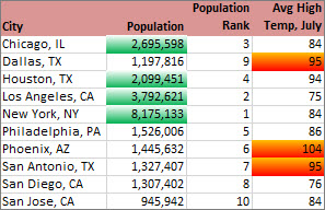
To more easily find specific cells, you can format them by using a comparison operator. For example, in an inventory worksheet sorted by categories, you could highlight products with fewer than 10 items on hand in yellow. Or, in a retail store summary worksheet, you might identify all stores with profits greater than 10%, sales volumes less than $100,000, and region equal to «SouthEast.»

The examples shown here work with examples of built-in conditional formatting criteria, such as Greater Than, and Top %. This formats cities with a population greater than 2,000,000 with a green background and average high temperatures in the top 30% with orange.

Note: You cannot conditionally format fields in the Values area of a PivotTable report by text or by date, only by number.

Quick formatting

Select one or more cells in a range, table, or PivotTable report.
On the Home tab, in the Style group, click the arrow next to Conditional Formatting, and then click Highlight Cells Rules.
Select the command you want, such as Between, Equal To Text that Contains, or A Date Occurring.
Enter the values you want to use, and then select a format.

You can change the method of scoping for fields in the Values area of a PivotTable report by using the Apply formatting rule to option button.

If you’d like to watch videos of these techniques, see Video: Conditionally format text and Video: Conditionally format dates.

Advanced formatting

Select one or more cells in a range, table, or PivotTable report.
On the Home tab, in the Styles group, click the arrow next to Conditional Formatting, and then click Manage Rules. The Conditional Formatting Rules Manager dialog box appears.
Do one of the following:
- To add a conditional format, click New Rule. The New Formatting Rule dialog box appears.
- To add a new conditional format based on one that is already listed, select the rule, then click Duplicate Rule. The duplicate rule is copied and appears in the dialog box. Select the duplicate, then select Edit Rule. The Edit Formatting Rule dialog box appears.
- To change a conditional format, do the following:
- 1. Make sure that the appropriate worksheet, table, or PivotTable report is selected in the Show formatting rules for list box.
  2. Optionally, change the range of cells by clicking Collapse Dialog in the Applies to box to temporarily hide the dialog box, by selecting the new range of cells on the worksheet or on other worksheets, and then by selecting Expand Dialog.
  3. Select the rule, and then click Edit rule. The Edit Formatting Rule dialog box appears.
Under Apply Rule To, to optionally change the scope for fields in the Values area of a PivotTable report by:
- Selection: Click Just these cells.
- Corresponding field: Click All <value field> cells with the same fields.
- Value field: Click All <value field> cells.
Under Select a Rule Type, click Format only cells that contain.
Under Edit the Rule Description, in the Format only cells with list box, do one of the following:
- Format by number, date, or time: Select Cell Value, select a comparison operator, and then enter a number, date, or time.
  
  For example, select Between and then enter 100 and 200, or select Equal to and then enter 1/1/2009.
  
  You can also enter a formula that returns a number, date, or time value.
  - If you enter a formula, start it with an equal sign (=).
  - Invalid formulas result in no formatting being applied.
  - It’s a good idea to test the formula to make sure that it doesn’t return an error value.
- Format by text: Select Specific Text, choosing a comparison operator, and then enter text.
  
  For example, select Contains and then enter Silver, or select Starting with and then enter Tri.
  
  Quotes are included in the search string, and you may use wildcard characters. The maximum length of a string is 255 characters.
  
  You can also enter a formula that returns text.
  - If you enter a formula, start it with an equal sign (=).
  - Invalid formulas result in no formatting being applied.
  - It’s a good idea to test the formula to make sure that it doesn’t return an error value.
  To see a video of this technique, see Video: Conditionally format text.
- Format by date: Select Dates Occurring and then select a date comparison.
  
  For example, select Yesterday or Next week.
  
  To see a video of this technique, see Video: Conditionally format dates.
- Format cells with blanks or no blanks: Select Blanks or No Blanks.
  
  A blank value is a cell that contains no data and is different from a cell that contains one or more spaces (spaces are considered as text).
- Format cells with error or no error values: Select Errors or No Errors.
  
  Error values include: #####, #VALUE!, #DIV/0!, #NAME?, #N/A, #REF!, #NUM!, and #NULL!.
To specify a format, click Format. The Format Cells dialog box appears.
Select the number, font, border, or fill format you want to apply when the cell value meets the condition, and then click OK.

You can choose more than one format. The formats you select are shown in the Preview box.

You can find the highest and lowest values in a range of cells that are based on a cutoff value you specify. For example, you can find the top 5 selling products in a regional report, the bottom 15% products in a customer survey, or the top 25 salaries in a department .

Quick formatting

Select one or more cells in a range, table, or PivotTable report.
On the Home tab, in the Style group, click the arrow next to Conditional Formatting, and then click Top/Bottom Rules.
Select the command you want, such as Top 10 items or Bottom 10 %.
Enter the values you want to use, and then select a format.

You can change the method of scoping for fields in the Values area of a PivotTable report by using the Apply formatting rule to option button.

Advanced formatting

Select one or more cells in a range, table, or PivotTable report.
On the Home tab, in the Styles group, click the arrow next to Conditional Formatting, and then click Manage Rules. The Conditional Formatting Rules Manager dialog box appears.
Do one of the following:
- To add a conditional format, click New Rule. The New Formatting Rule dialog box appears.
- To add a new conditional format based on one that is already listed, select the rule, then click Duplicate Rule. The duplicate rule is copied and appears in the dialog box. Select the duplicate, then select Edit Rule. The Edit Formatting Rule dialog box appears.
- To change a conditional format, do the following:
- 1. Make sure that the appropriate worksheet, table, or PivotTable report is selected in the Show formatting rules for list box.
  2. Optionally, change the range of cells by clicking Collapse Dialog in the Applies to box to temporarily hide the dialog box, by selecting the new range of cells on the worksheet, and then by selecting Expand Dialog.
  3. Select the rule, and then click Edit rule. The Edit Formatting Rule dialog box appears.
Under Apply Rule To, to optionally change the scope fields in the Values area of a PivotTable report by:
- Selection: Click Just these cells.
- Corresponding field: Click All <value field> cells with the same fields.
- Value field: Click All <value field> cells.
Under Select a Rule Type, click Format only top or bottom ranked values.
Under Edit the Rule Description, in the Format values that rank in the list box, select Top or Bottom.
Do one of the following:
- To specify a top or bottom number, enter a number and then clear the % of the selected range box. Valid values are 1 to 1000.
- To specify a top or bottom percentage, enter a number and then select the % of the selected range box. Valid values are 1 to 100.
Optionally, change how the format is applied for fields in the Values area of a PivotTable report that are scoped by corresponding field.

By default, the conditional format is based on all visible values. However when you scope by corresponding field, instead of using all visible values, you can apply the conditional format for each combination of:
- A column and its parent row field, by selecting each Column group.
- A row and its parent column field, by selecting each Row group.
To specify a format, click Format. The Format Cells dialog box appears.
Select the number, font, border, or fill format you want to apply when the cell value meets the condition, and then click OK.

You can choose more than one format. The formats you select are shown in the Preview box.

You can find values above or below an average or standard deviation in a range of cells. For example, you can find the above average performers in an annual performance review or you can locate manufactured materials that fall below two standard deviations in a quality rating.

Quick formatting

Select one or more cells in a range, table, or PivotTable report.
On the Home tab, in the Style group, click the arrow next to Conditional Formatting, and then click Top/Bottom Rules.
Select the command you want, such as Above Average or Below Average.
Enter the values you want to use, and then select a format.

You can change the method of scoping for fields in the Values area of a PivotTable report by using the Apply formatting rule to option button.

Advanced formatting

Select one or more cells in a range, table, or PivotTable report.
On the Home tab, in the Styles group, click the arrow next to Conditional Formatting, and then click Manage Rules. The Conditional Formatting Rules Manager dialog box appears.
Do one of the following:
- To add a conditional format, click New Rule. The New Formatting Rule dialog box appears.
- To add a new conditional format based on one that is already listed, select the rule, then click Duplicate Rule. The duplicate rule is copied and appears in the dialog box. Select the duplicate, then select Edit Rule. The Edit Formatting Rule dialog box appears.
- To change a conditional format, do the following:
- 1. Make sure that the appropriate worksheet, table, or PivotTable report is selected in the Show formatting rules for list box.
  2. Optionally, change the range of cells by clicking Collapse Dialog in the Applies to box to temporarily hide the dialog box, by selecting the new range of cells on the worksheet, and then by selecting Expand Dialog.
  3. Select the rule, and then click Edit rule. The Edit Formatting Rule dialog box appears.
Under Apply Rule To, to optionally change the scope for fields in the Values area of a PivotTable report by:
- Selection: Click Just these cells.
- Corresponding field: Click All <value field> cells with the same fields.
- Value field: Click All <value field> cells.
Under Select a Rule Type, click Format only values that are above or below average.
Under Edit the Rule Description, in the Format values that are list box, do one of the following:
- To format cells that are above or below the average for all of the cells in the range, select Above or Below.
- To format cells that are above or below one, two, or three standard deviations for all of the cells in the range, select a standard deviation.
Optionally, change how the format is applied for fields in the Values area of a PivotTable report that are scoped by corresponding field.

By default, the conditionally format is based on all visible values. However when you scope by corresponding field, instead of using all visible values, you can apply the conditional format for each combination of:
- A column and its parent row field, by selecting each Column group.
- A row and its parent column field, by selecting each Row group.
Click Format to display the Format Cells dialog box.
Select the number, font, border, or fill format you want to apply when the cell value meets the condition, and then click OK.

You can choose more than one format. The formats you select are displayed in the Preview box.

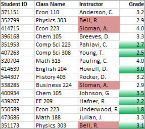
Note: You can’t conditionally format fields in the Values area of a PivotTable report by unique or duplicate values.

In the example shown here, conditional formatting is used on the Instructor column to find instructors that are teaching more than one class (duplicate instructor names are highlighted in a pale red color). Grade values that are found just once in the Grade column (unique values) are highlighted in a green color.

Quick formatting

Select the cells that you want to conditionally format.
On the Home tab, in the Style group, click the arrow next to Conditional Formatting, and then click Highlight Cells Rules.
Select Duplicate Values.
Enter the values you want to use, and then select a format.

Advanced formatting

Select the cells that you want to conditionally format.
On the Home tab, in the Styles group, click the arrow next to Conditional Formatting, and then click Manage Rules. The Conditional Formatting Rules Manager dialog box appears.
Do one of the following:
- To add a conditional format, click New Rule. The New Formatting Rule dialog box appears.
- To add a new conditional format based on one that is already listed, select the rule, then click Duplicate Rule. The duplicate rule is copied and appears in the dialog box. Select the duplicate, then select Edit Rule. The Edit Formatting Rule dialog box appears.
- To change a conditional format, do the following:
- 1. Make sure that the appropriate worksheet or table is selected in the Show formatting rules for list box.
  2. Optionally, change the range of cells by clicking Collapse Dialog in the Applies to box to temporarily hide the dialog box, by selecting the new range of cells on the worksheet, and then by selecting Expand Dialog.
  3. Select the rule, and then click Edit rule. The Edit Formatting Rule dialog box appears.
Under Select a Rule Type, click Format only unique or duplicate values.
Under Edit the Rule Description, in the Format all list box, select unique or duplicate.
Click Format to display the Format Cells dialog box.
Select the number, font, border, or fill format you want to apply when the cell value meets the condition, and then click OK.

You can choose more than one format. The formats you select are shown in the Preview box.

If none of the above options is what you’re looking for, you can create your own conditional formatting rule in a few simple steps.

Notes: If there’s already a rule defined that you just want to work a bit differently, duplicate the rule and edit it.

Select Home > Conditional Formatting > Manage Rules, then in the Conditional Formatting Rule Manager dialog, select a listed rule and then select Duplicate Rule. The duplicate rule then appears in the list.
Select the duplicate rule, then select Edit Rule.

Select the cells that you want to format.
On the Home tab, click Conditional Formatting > New Rule.
Create your rule and specify its format options, then click OK.

If you don’t see the options that you want, you can use a formula to determine which cells to format — see the next section for steps).

If you don’t see the exact options you need when you create your own conditional formatting rule, you can use a logical formula to specify the formatting criteria. For example, you may want to compare values in a selection to a result returned by a function or evaluate data in cells outside the selected range, which can be in another worksheet in the same workbook. Your formula must return True or False (1 or 0), but you can use conditional logic to string together a set of corresponding conditional formats, such as different colors for each of a small set of text values (for example, product category names).

Note: You can enter cell references in a formula by selecting cells directly on a worksheet or other worksheets. Selecting cells on the worksheet inserts absolute cell references. If you want Excel to adjust the references for each cell in the selected range, use relative cell references. For more information, see Create or change a cell reference and Switch between relative, absolute, and mixed references.

Tip: If any cells contain a formula that returns an error, conditional formatting is not applied to those cells. To address this, use IS functions or an IFERROR function in your formula to return a value that you specify (such as 0, or «N/A») instead of an error value.

On the Home tab, in the Styles group, click the arrow next to Conditional Formatting, and then click Manage Rules.

The Conditional Formatting Rules Manager dialog box appears.
Do one of the following:
- To add a conditional format, click New Rule. The New Formatting Rule dialog box appears.
- To add a new conditional format based on one that is already listed, select the rule, then click Duplicate Rule. The duplicate rule is copied and appears in the dialog box. Select the duplicate, then select Edit Rule. The Edit Formatting Rule dialog box appears.
- To change a conditional format, do the following:
- 1. Make sure that the appropriate worksheet, table, or PivotTable report is selected in the Show formatting rules for list box.
  2. Optionally, change the range of cells by clicking Collapse Dialog in the Applies to box to temporarily hide the dialog box, by selecting the new range of cells on the worksheet or other worksheets, and then by clicking Expand Dialog.
  3. Select the rule, and then click Edit rule. The Edit Formatting Rule dialog box appears.
Under Apply Rule To, to optionally change the scope for fields in the Values area of a PivotTable report, do the following:
- To scope by selection: Click Selected cells.
- To scope by corresponding field: Click All cells showing <Values field> values.
- To scope by Value field: Click All cells showing <Values field> for <Row>.

Under Select a Rule Type, click Use a formula to determine which cells to format.

Under Edit the Rule Description, in the Format values where this formula is true list box, enter a formula.

You have to start the formula with an equal sign (=), and the formula must return a logical value of TRUE (1) or FALSE (0).
Click Format to display the Format Cells dialog box.

Select the number, font, border, or fill format you want to apply when the cell value meets the condition, and then click OK.

You can choose more than one format. The formats you select are shown in the Preview box.

Example 1: Use two conditional formats with criteria that uses AND and OR tests

The following example shows the use of two conditional formatting rules. If the first rule doesn’t apply, the second rule applies.

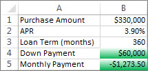
First rule: a home buyer has budgeted up to $75,000 as a down payment and $1,500 per month as a mortgage payment. If both the down payment and the monthly payments fit these requirements, cells B4 and B5 are formatted green.

Second rule: if either the down payment or the monthly payment doesn’t meet the buyer’s budget, B4 and B5 are formatted red. Change some values, such as the APR, the loan term, the down payment, and the purchase amount to see what happens with the conditionally formatted cells.

Formula for first rule (applies green color)	=AND(IF($B$4<=75000,1),IF(ABS($B$5)<=1500,1))
Formula for second rule (applies red color)	=OR(IF($B$4>=75000,1),IF(ABS($B$5)>=1500,1))

Example 2: Shade every other row by using the MOD and ROW functions

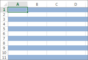
A conditional format applied to every cell in this worksheet shades every other row in the range of cells with a blue cell color. You can select all cells in a worksheet by clicking the square above row 1 and to the left of column A. The MOD function returns a remainder after a number (the first argument) is divided by divisor (the second argument). The ROW function returns the current row number. When you divide the current row number by 2, you always get either a 0 remainder for an even number or a 1 remainder for an odd number. Because 0 is FALSE and 1 is TRUE, every odd numbered row is formatted. The rule uses this formula: =MOD(ROW(),2)=1.

The following video shows you the basics of using formulas with conditional formatting.

If you want to apply an existing formatting style to new or other data on your worksheet, you can use Format Painter to copy the conditional formatting to that data.

Click the cell that has the conditional formatting that you want to copy.
Click Home > Format Painter.

The pointer changes to a paintbrush.

Tip: You can double-click Format Painter if you want to keep using the paintbrush to paste the conditional formatting in other cells.
To paste the conditional formatting, drag the paintbrush across the cells or ranges of cells you want to format.
To stop using the paintbrush, press Esc.

Note: If you’ve used a formula in the rule that applies the conditional formatting, you might have to adjust any cell references in the formula after pasting the conditional format. For more information, see Switch between relative, absolute, and mixed references.

If your worksheet contains conditional formatting, you can quickly locate the cells so that you can copy, change, or delete the conditional formats. Use the Go To Special command to find only cells with a specific conditional format, or to find all cells that have conditional formats.

Find all cells that have a conditional format

Click any cell that does not have a conditional format.
On the Home tab, in the Editing group, click the arrow next to Find & Select, and then click Conditional Formatting.

Find only cells that have the same conditional format

Click any cell that has the conditional format that you want to find.
On the Home tab, in the Editing group, click the arrow next to Find & Select, and then click Go To Special.
Click Conditional formats.
Click Same under Data validation.

When you use conditional formatting, you set up rules that Excel uses to determine when to apply the conditional formatting. To manage these rules, you should understand the order in which these rules are evaluated, what happens when two or more rules conflict, how copying and pasting can affect rule evaluation, how to change the order in which rules are evaluated, and when to stop rule evaluation.

Learn about conditional formatting rule precedence

You create, edit, delete, and view all conditional formatting rules in the workbook by using the Conditional Formatting Rules Manager dialog box. (On the Home tab, click Conditional Formatting, and then click Manage Rules.)

The Conditional Formatting Rules Manager dialog box appears.

When two or more conditional formatting rules apply, these rules are evaluated in order of precedence (top to bottom) by how they are listed in this dialog box.

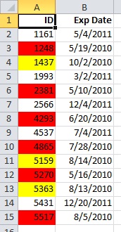
Here’s an example that has expiration dates for ID badges. We want to mark badges that expire within 60 days but are not yet expired with a yellow background color, and expired badges with a red background color.

In this example, cells with employee ID numbers who have certification dates due to expire within 60 days are formatted in yellow, and ID numbers of employees with an expired certification are formatted in red. The rules are shown in the following image.

The first rule (which, if True, sets cell background color to red) tests a date value in column B against the current date (obtained by using the TODAY function in a formula). Assign the formula to the first data value in column B, which is B2. The formula for this rule is =B2<TODAY(). This formula tests the cells in column B (cells B2:B15). If the formula for any cell in column B evaluates to True, its corresponding cell in column A (for example, A5 corresponds to B5, A11 corresponds to B11), is then formatted with a red background color. After all the cells specified under Applies to are evaluated with this first rule, the second rule is tested. This formula checks if values in the B column are less than 60 days from the current date (for example, suppose today’s date is 8/11/2010). The cell in B4, 10/4/2010, is less than 60 days from today, so it evaluates as True, and is formatted with a yellow background color. The formula for this rule is =B2<TODAY()+60. Any cell that was first formatted red by the highest rule in the list is left alone.

A rule higher in the list has greater precedence than a rule lower in the list. By default, new rules are always added to the top of the list and therefore have a higher precedence, so you’ll want to keep an eye on their order. You can change the order of precedence by using the Move Up and Move Down arrows in the dialog box.
What happens when more than one conditional formatting rule evaluates to True

Sometimes you have more than one conditional formatting rule that evaluates to True. Here’s how rules are applied, first when rules don’t conflict, and then when they do conflict:

When rules don’t conflict For example, if one rule formats a cell with a bold font and another rule formats the same cell with a red color, the cell is formatted with both a bold font and a red color. Because there is no conflict between the two formats, both rules are applied.

When rules conflict For example, one rule sets a cell font color to red and another rule sets a cell font color to green. Because the two rules are in conflict, only one can apply. The rule that is applied is the one that is higher in precedence (higher in the list in the dialog box).
How pasting, filling, and the Format Painter affect conditional formatting rules

While editing your worksheet, you may copy and paste cell values that have conditional formats, fill a range of cells with conditional formats, or use the Format Painter. These operations can affect conditional formatting rule precedence in the following way: a new conditional formatting rule based on the source cells is created for the destination cells.

If you copy and paste cell values that have conditional formats to a worksheet opened in another instance of Excel (another Excel.exe process running at the same time on the computer), no conditional formatting rule is created in the other instance and the format is not copied to that instance.
What happens when a conditional format and a manual format conflict

If a conditional formatting rule evaluates as True, it takes precedence over any existing manual format for the same selection. This means that if they conflict, the conditional formatting applies and the manual format does not. If you delete the conditional formatting rule, the manual formatting for the range of cells remains.

Manual formatting is not listed in the Conditional Formatting Rules Manager dialog box nor is it used to determine precedence.

Controlling when rule evaluation stops by using the Stop If True check box

For backwards compatibility with versions of Excel earlier than Excel 2007, you can select the Stop If True check box in the Manage Rules dialog box to simulate how conditional formatting might appear in those earlier versions of Excel that do not support more than three conditional formatting rules or multiple rules applied to the same range.

For example, if you have more than three conditional formatting rules for a range of cells, and are working with a version of Excel earlier than Excel 2007, that version of Excel:

Evaluates only the first three rules.
Applies the first rule in precedence that is True.
Ignores rules lower in precedence if they are True.

The following table summarizes each possible condition for the first three rules:

If rule	Is	And if rule	Is	And if rule	Is	Then
One	True	Two	True or False	Three	True or False	Rule one is applied and rules two and three are ignored.
One	False	Two	True	Three	True or False	Rule two is applied and rule three is ignored.
One	False	Two	False	Three	True	Rule three is applied.
One	False	Two	False	Three	False	No rules are applied.

You can select or clear the Stop If True check box to change the default behavior:

To evaluate only the first rule, select the Stop If True check box for the first rule.
To evaluate only the first and second rules, select the Stop If True check box for the second rule.

You can’t select or clear the Stop If True check box if the rule formats by using a data bar, color scale, or icon set.

If you’d like to watch a video showing how to manage conditional formatting rules, see Video: Manage conditional formatting.

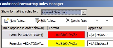
The order in which conditional formatting rules are evaluated — their precedence — also reflects their relative importance: the higher a rule is on the list of conditional formatting rules, the more important it is. This means that in cases where two conditional formatting rules conflict with each other, the rule that is higher on the list is applied and the rule that is lower on the list is not applied.

On the Home tab, in the Styles group, click the arrow next to Conditional Formatting, and then click Manage Rules.

The Conditional Formatting Rules Manager dialog box appears.

The conditional formatting rules for the current selection are displayed, including the rule type, the format, the range of cells the rule applies to, and the Stop If True setting.

If you don’t see the rule that you want, in the Show formatting rules for list box, make sure that the right range of cells, worksheet, table, or PivotTable report is selected.
Select a rule. Only one rule can be selected at a time.
To move the selected rule up in precedence, click Move Up. To move the selected rule down in precedence, click Move Down.
Optionally, to stop rule evaluation at a specific rule, select the Stop If True check box.

Clear conditional formatting on a worksheet

On the Home tab, click Conditional Formatting > Clear Rules > Clear Rules from Entire Sheet.

Follow these steps if you have conditional formatting in a worksheet, and you need to remove it.

For an entire
worksheet

On the Home tab, click Conditional Formatting > Clear Rules > Clear Rules from Entire Sheet.

In a range of cells

Select the cells that contain the conditional formatting.
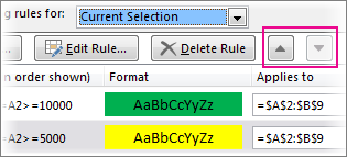
Click the Quick Analysis Lens button that appears to the bottom right of the selected data.
Notes:
Quick Analysis Lens will not be visible if:
- All of the cells in the selected range are empty, or
- There is an entry only in the upper-left cell of the selected range, with all of the other cells in the range being empty.
Click Clear Format.

Find and remove the same conditional formats throughout a worksheet

Click on a cell that has the conditional format that you want to remove throughout the worksheet.
On the Home tab, click the arrow next to Find & Select, and then click Go To Special.
Click Conditional formats.
Click Same under Data validation. to select all of the cells that contain the same conditional formatting rules.
On the Home tab, click Conditional Formatting > Clear Rules > Clear Rules from Selected Cells.

Tip: The following sections use examples so you can follow along in Excel for the web. To start, download the Conditional Formatting Examples workbook and save it to OneDrive. Then, open OneDrive in a web browser and select the downloaded file.

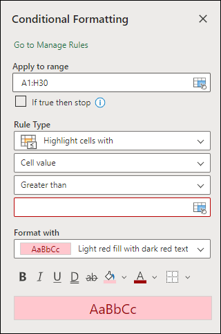
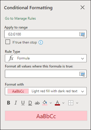
Select the cells you want to format, then select Home > Styles > Conditional Formatting > New Rule. You can also open the Conditional Formatting pane and create a new rule without first selecting a range of cells.
Verify or adjust the cells in Apply to range.
Choose a Rule Type and adjust the options to meet your needs.
When finished, select Done and the rule will be applied to your range.

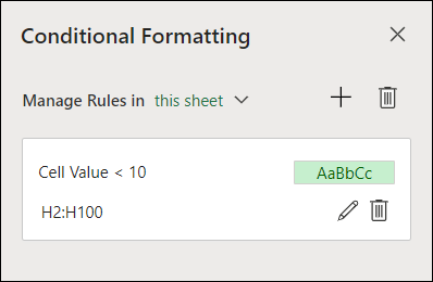
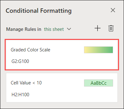
Select a cell which has a conditional format you want to change. Or you can select Home > Styles > Conditional Formatting > Manage Rules to open the Conditional Formatting task pane and select an existing rule.
The Conditional Formatting task pane displays any rules which apply to specific cells or ranges of cells.
Hover over the rule and select Edit by clicking the pencil icon. This opens the task pane for rule editing.
Modify the rule settings and click Done to apply the changes.

The Conditional Formatting task pane provides everything you need for creating, editing, and deleting rules. Use Manage Rules to open the task pane and work with all the Conditional Formatting rules in a selection or a sheet.

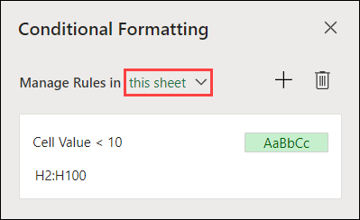
In an open workbook, select Home > Styles > Conditional Formatting > Manage Rules.
The Conditional Formatting task pane opens and displays the rules, scoped to your current selection.

From here, you can:

Choose a different scope on the Manage Rules in menu — for example, choosing this sheet tells Excel to look for all rules on the current sheet.
Add a rule by selecting New Rule (the plus sign).
Delete all rules in scope by selecting Delete All Rules (the garbage can).

You can use a formula to determine how Excel evaluates and formats a cell. Open the Conditional Formatting pane and select an existing rule or create a new rule.

In the Rule Type dropdown, select Formula.

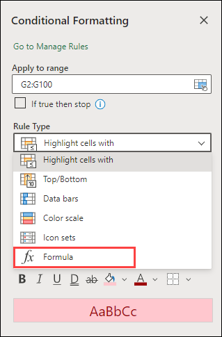
Enter the formula in the box. You can use any formula that returns a logical value of TRUE (1) or FALSE (0), but you can use AND and OR to combine a set of logical checks.

For example, =AND(B3=»Grain»,D3<500) is true for a cell in row 3 if both B3=»Grain» and D3<500 are true.

You can clear conditional formatting in selected cells or the entire worksheet.

To clear conditional formatting in selected cells, select the cells in the worksheet. Then Select Home > Styles > Conditional Formatting > Clear Rules > Clear Rules from Selected Cells.
To clear conditional formatting in the entire worksheet, select Home > Styles > Conditional Formatting > Clear Rules > Clear Rules from Entire Sheet.
To delete conditional formatting rules, select Home > Styles > Conditional Formatting >Manage Rules and use the delete (garbage can) on a specific rule or the Delete all rules button.

Color scales are visual guides which help you understand data distribution and variation. Excel offers both two-color scales and three-color scales.

A two-color scale helps you compare a range of cells by using a gradation of two colors. The shade of the color represents higher or lower values. For example, in a green and yellow color scale, you can specify that higher value cells be more green and lower value cells have a more yellow.

A three-color scale helps you compare a range of cells by using a gradation of three colors. The shade of the color represents higher, middle, or lower values. For example, in a green, yellow, and red color scale, you can specify that higher value cells have a green color, middle value cells have a yellow color, and lower value cells have a red color.

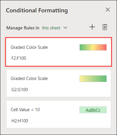
Tip: You can sort cells that have one of these formats by their color — just use the context menu.

Select the cells that you want to conditionally format using color scales.
Click Home > Styles > Conditional Formatting > Color Scales and select a color scale.

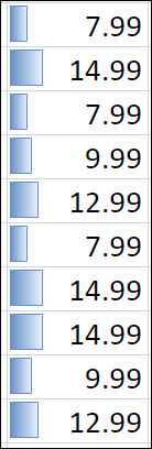
A data bar helps you see the value of a cell relative to other cells. The length of the data bar represents the value in the cell. A longer bar represents a higher value, and a shorter bar represents a lower value. Data bars are useful in spotting higher and lower numbers, especially with large amounts of data, such as top selling and bottom selling toys in a holiday sales report.

Select the cells that you want to conditionally format.
Select Home > Styles > Conditional Formatting > Data Bars and select a style.

Use an icon set to annotate and classify data into three to five categories separated by a threshold value. Each icon represents a range of values. For example, in the 3 Arrows icon set, the green up arrow represents higher values, the yellow sideways arrow represents middle values, and the red down arrow represents lower values.

Select the cells that you want to conditionally format.
Select Home > Styles > Conditional Formatting > Icon Sets and choose an icon set.

This option lets you highlight specific cell values within a range of cells based on their specific contents. This can be especially useful when working with data sorted using a different range.

For example, in an inventory worksheet sorted by categories, you could highlight the names of products where you have fewer than 10 items in stock so it’s easy to see which products need restocking without resorting the data.

Select the cells that you want to conditionally format.
Select Home > Styles > Conditional Formatting > Highlight Cell Rules.
Select the comparison, such as Between, Equal To, Text That Contains, or A Date Occurring.

You can highlight the highest and lowest values in a range of cells which are based on a specified cutoff value.

Some examples of this would include highlighting the top five selling products in a regional report, the bottom 15% products in a customer survey, or the top 25 salaries in a department.

Select the cells that you want to conditionally format.
Select Home > Styles > Conditional Formatting > Top/Bottom Rules.
Select the command you want, such as Top 10 items or Bottom 10 %.
Enter the values you want to use, and select a format (fill, text, or border color).

You can highlight values above or below an average or standard deviation in a range of cells.

For example, you can find the above-average performers in an annual performance review, or locate manufactured materials that fall below two standard deviations in a quality rating.

Select the cells that you want to conditionally format.
Select Home> Styles > Conditional Formatting > Top/Bottom Rules.
Select the option you want, such as Above Average or Below Average.
Enter the values you want to use, and select a format (fill, text, or border color).

Select the cells that you want to conditionally format.
Select Home > Styles > Conditional Formatting > Highlight Cell Rules > Duplicate Values.
Enter the values you want to use, and select a format (fill, text, or border color).

If you want to apply an existing formatting style to other cells on your worksheet, use Format Painter to copy the conditional formatting to that data.

Click the cell that has the conditional formatting you want to copy.
Click Home > Format Painter.

The pointer will change to a paintbrush.

Tip: You can double-click Format Painter if you want to keep using the paintbrush to paste the conditional formatting in other cells.
Drag the paintbrush across the cells or range of cells you want formatted.
To stop using the paintbrush, press Esc.

Note: If you’ve used a formula in the rule that applies the conditional formatting, you might have to adjust relative and absolute references in the formula after pasting the conditional format. For more information, see Switch between relative, absolute, and mixed references.

Note: You can’t use conditional formatting on external references to another workbook.

Need more help?

You can always ask an expert in the Excel Tech Community or get support in the Answers community.

What Is Conditional Formatting?

Conditional formatting is a feature of many spreadsheet applications that allows you to apply special formatting to cells that meet certain criteria. It is most often used to highlight, emphasize, or differentiate among data and information stored in a spreadsheet.

Conditional formatting enables spreadsheet users to do a number of things. First and foremost, it calls attention to important data points such as deadlines, at-risk tasks, or budget items. It can also make large data sets more digestible by breaking up the wall of numbers with a visual organizational component. Finally, conditional formatting can transform your spreadsheet (that previously only stored data) into a dependable “alert” system that highlights key information and keeps you on top of your workload.

Originally a powerful feature of Excel, other spreadsheet applications have also adopted this functionality.

Conditional Formatting Basics

Conditional formatting consists of four main components: if-then commands, preset conditions, custom conditions, and applying multiple conditions. We’ve outlined how to use these commands and conditions to create and apply rules to your Excel spreadsheets below:

If-Then Logic: All conditional formatting rules are based on simple if-then logic: if X criteria is true, then Y formatting will be applied (this is often written as p → q, or if p is true, then apply q). You won’t have to hard-code any logic, though — Excel and other spreadsheet apps have built-in parameters so you can simply select the conditions you want the rules to meet. Advanced users can also apply the program’s built-in formulas to logic rules.
Preset Conditions: Excel has a huge library of preset rules encompassing nearly all functions that beginner users will want to apply. We’ll familiarize you with several of the most popular ones in the next section.
Custom Conditions: For situations where you want to manipulate a preset condition, you can create your own rules. If appropriate, you can use Excel formulas in the rules you write.
Applying Multiple Conditions: You can apply multiple rules to a single cell or range of cells. However, be aware of rule hierarchy and precedence — we’ll show you how to manage stacked rules in the walkthrough.

Overall, applying conditional formatting is an easy way to keep you and your team members up to date with your data — calling visual attention to important dates and deadlines, tasks and assignments, budget constraints, and anything else you might want to highlight. When applied correctly, conditional formatting will make you more productive by reducing time spent manually combing data and making it easier to identify trends, so you can focus on the big decisions.

How to Apply Basic Conditional Formatting in Excel

You can apply conditional formatting to your Excel spreadsheets using various tools and features found within the program. This step-by-step walkthrough shows you how to apply the most commonly used formatting for highlighting, data bars, color scales, and more.

Step 1: Apply Highlight Rules to Your Excel Spreadsheet

Highlight rules apply color formatting to cells that meet specific criteria that you define. They are the most basic type of conditional formatting rule, and Excel provides a variety of preset highlight functions.

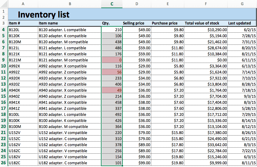
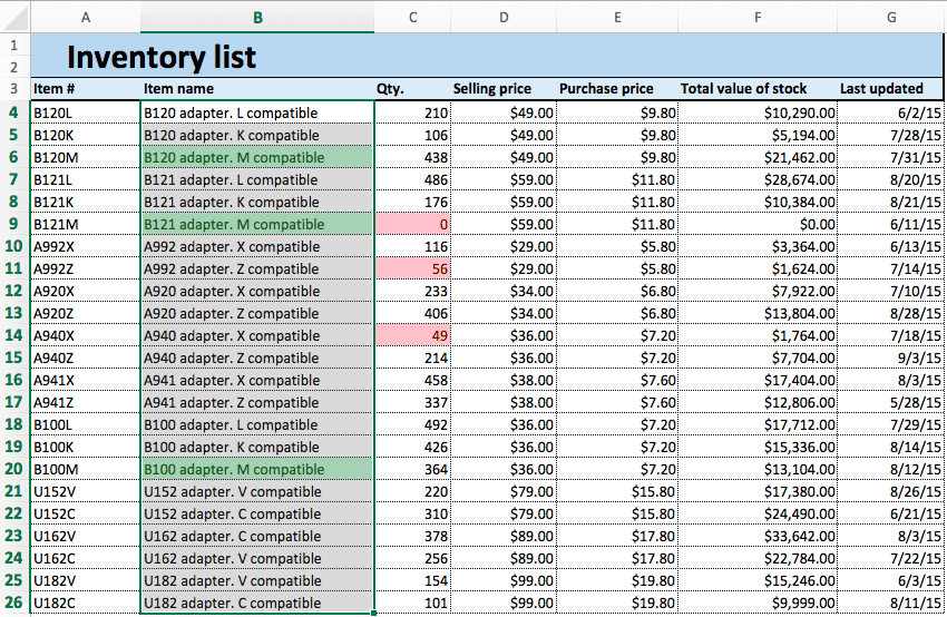
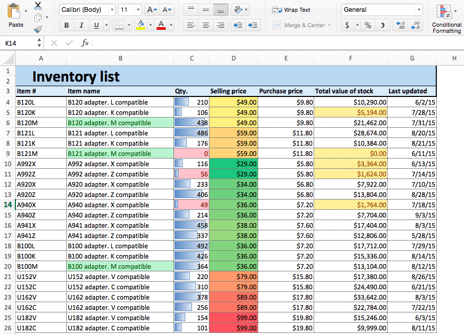
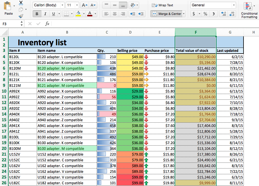
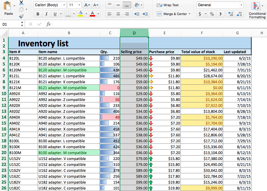
Open an existing spreadsheet in Excel, or start from scratch and manually enter new data. In this example, we’re using an inventory list that tracks the number of each item currently in stock, as well as some additional information about each product.
To apply highlight rules, select the range of values you want to apply a rule to. For this example, we want to highlight any product that’s quantity is less than 100 units. So, select the values in the Qty. column (C4:C26).
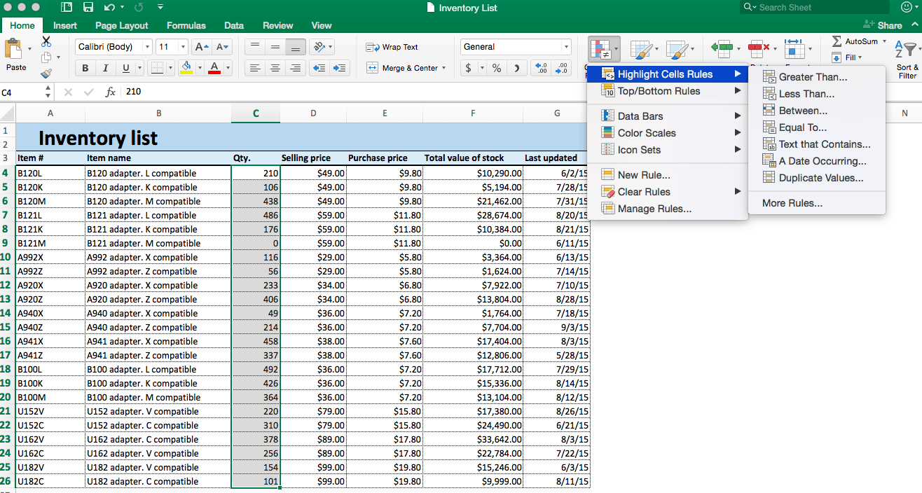
From the Home tab, click Conditional Formatting on the right side of the toolbar, and click Highlight Cells Rules from the dropdown menu. Click Less than.
A box will appear. Type 100 in the empty field. Click OK.
Your spreadsheet will now reflect this highlight rule, with the quantities less than 100 highlighted red with red text.
Tip: You can change the color of the highlighted cell by clicking on the Format with: dropdown menu and selecting on another option.
To highlight text cells, repeat step 2. This time, we want to highlight certain model types (M compatible), so we’ll select the cells in the Item name column.
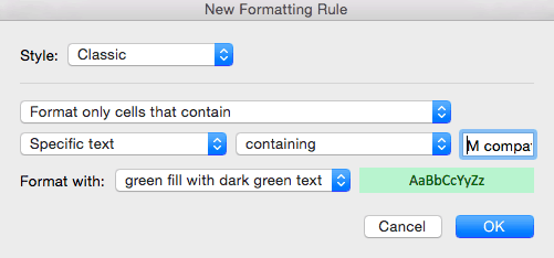
Click Conditional Formatting > Highlight Cells Rules > Text that Contains…
Type M compatible in the text box. To differentiate from our previous highlight rule, select green fill with dark green text from the Format with: dropdown menu. Click OK.
Now, cells containing the text M compatible are highlighted.

Using these same steps and menu options, you can apply highlight rules to find Duplicate Values, Dates, or values that are Greater than…, Equal to…, or Between… values that you select. All of these possibilities are available through the menu options.

Step 2: Create Top/Bottom Rules

Step 3: Apply Data Bars

Data bars apply a visual bar within each cell. The length of the bar relates the value of the cell to other cell values in the selected range.

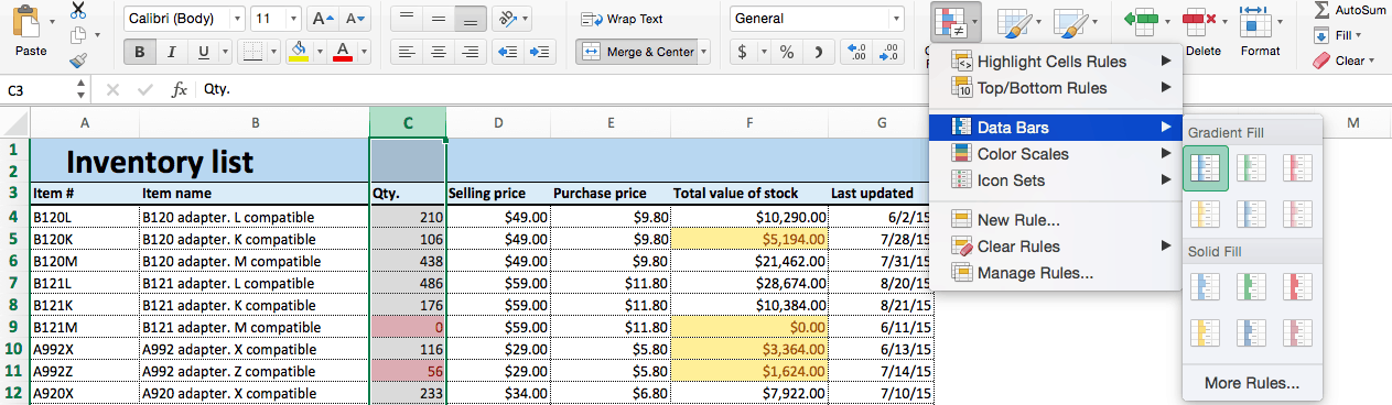
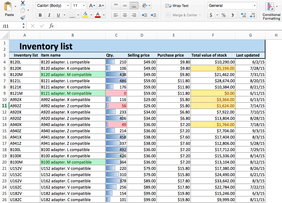
We’ll apply data bars to the Qty. column so we can easily assess the ratios of items in stock. Click the top of the Qty. column to select this range of cells.
Click Conditional Formatting > Data Bars. You’ll see two options — one for Gradient Fill and one for Solid Fill. They function identically; just select the option and color you prefer.
Your sheet will now reflect the added rule.

Step 4: Apply Color Scales

Color scales are similar to data bars in that they relate a cell’s values in a selected range. However, instead of representing this relationship by the length of a bar, color scales do so with color gradients. One color is assigned the “lowest” value and another the “highest,” with a range of colors in between.

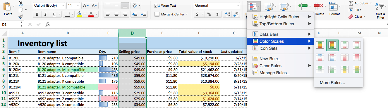
We’ll apply color scales to our Selling price column. Click the top of column D to select this range.
Click Conditional Formatting > Color Scales. You’ll see a variety of different color ranges; select the one you want.
Your spreadsheet now shows the selling prices by color — red cells are the most expensive, and green cells are the least expensive.

Step 5: Apply Icon Sets

Icon sets apply colorful icons to data. They are simply another way to call attention to important data, and relate cells to one another.

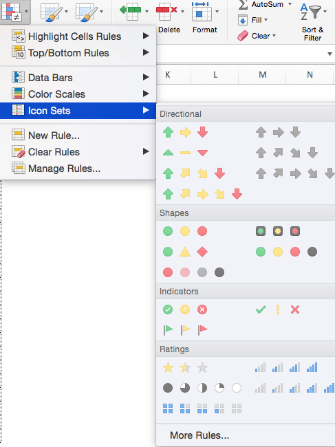
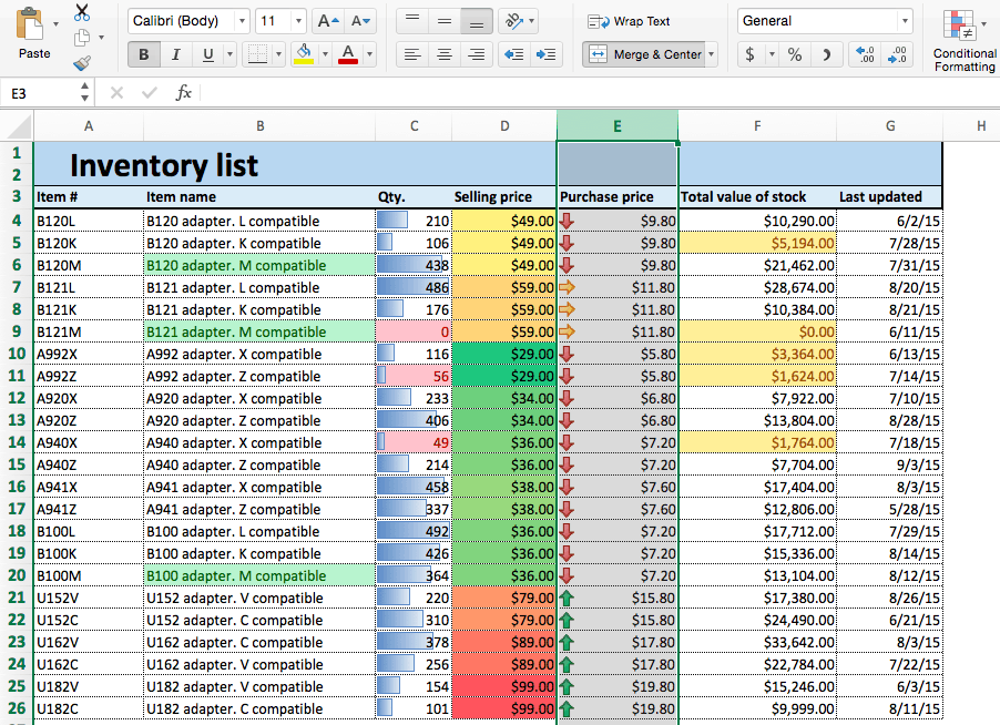
We’ll apply icon sets to the Purchase price column to show low, middle, and high priced items. Click the top of the Purchase price column to select the range of values.
Click Conditional Formatting > Icon Sets. You’ll see a variety of options for Directional, Shapes, Indicators, and Ratings icons. You can choose any of these to fit the needs of your data. In this example, we’ll choose the first Directional option: red, yellow, and green arrows that indicate high, middle, or low priced items.
Your sheet reflects this new formatting rule.

Step 6: Edit and Delete Conditional Formatting Rules

Now you’ve learned the most common conditional formatting presets in Excel, your spreadsheet provides a lot of information at a glance. However, you might want to edit some of these rules later on, or delete them completely.

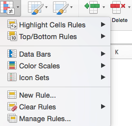
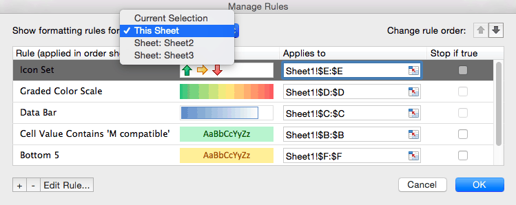
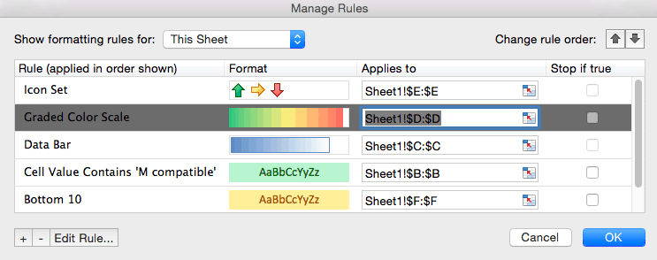
Click Conditional Formatting and select Manage Rules… from the dropdown list.
The Manage Rules box will appear. Click the dropdown menu at the top of the box and click This Sheet to list the conditional formatting rules you have applied to the current sheet.
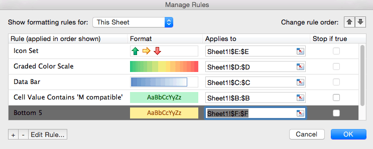
To edit a rule, click the rule you want to change. In this example, we want to highlight the bottom ten values in the Total value of stock column, rather than the bottom five that we currently have highlighted. Click the Bottom 5 row. Then, click Edit Rule… at the bottom of the box.
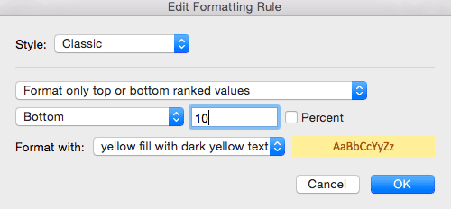
A new box opens where you can adjust the conditions of the rule. Type 10 in the number field and click OK.
Excel will bring you back to the Manage Rules box. You must click OK to save the changes you made to the original rule.
To delete a rule, return to the Manage Rules box and choose This Sheet. Click the rule you want to delete — in this case, the color grading on Selling price. Click the — symbol (next to Edit Rule…) in the lower left hand corner. Click OK.
The conditional formatting on the Selling price column is now deleted.

You now have everything need to create basic conditional formatting using presets in Excel 2016. For more advanced functionality such as creating a new rule, using Excel formulas, and creating rules dependent on another cell, see the “Advanced” section below.

First, we’ll look at how we can apply the same conditional formatting rules we learned in Excel to another spreadsheet program, Smartsheet.

How to Apply Basic Conditional Formatting in Smartsheet

Use conditional formatting in Smartsheet to apply many of the same rules and effects available in Excel. We’ll guide you through every function described in the previous section, with some modifications that better align with Smartsheet features.

You can create spreadsheets in Smartsheet two ways: by manually entering data into Smartsheet, or by importing an existing spreadsheet from programs like Excel and MS Project. For this tutorial, we’ll use the same data set from the Excel tutorial, so we’ll import the original version (with no conditional formatting) from Excel.

Step 1: Open Your Existing Excel Spreadsheet in Smartsheet

Step 2: Apply Highlight Rules

To highlight a cell, click the conditional formatting icon on the toolbar.
A box will appear where you can set conditional formatting rules. Click Add New Rule in the top left corner. The if-then logic is already written into the new rule, so you can simply create the conditions.
Click set condition. Just like in the Excel example, we want to highlight any items that are stocked below 100 units. Select Qty. from the column list on the left, select is less than from the center dropdown list, and then type 100 in the field on the right. Click OK.
Now we need to apply the formatting. Click this format and a dropdown menu with formatting options appears. For this example, we’ll use a paint fill. Click the paint bucket icon and select red.
Specify which cells should get this formatting. Smartsheet will default to format the entire row, but we only want to highlight the cells in the Qty. column. Click entire row and click Qty. from the dropdown list. Click OK.
Your conditional formatting rule is now reflected in your spreadsheet.
To highlight text cells, repeat steps 1 and 2. Click set condition. Now, we want to highlight any M compatible items. Select Item name from the left-most list, contains from the center list, and type M compatible in the right field. Click OK.
Click this format and click the paint bucket item. Select green. For this rule, we want to highlight the entire row. (Again, Smartsheet defaults to this option.) Click OK.
Your second rule is now reflected in your data set.

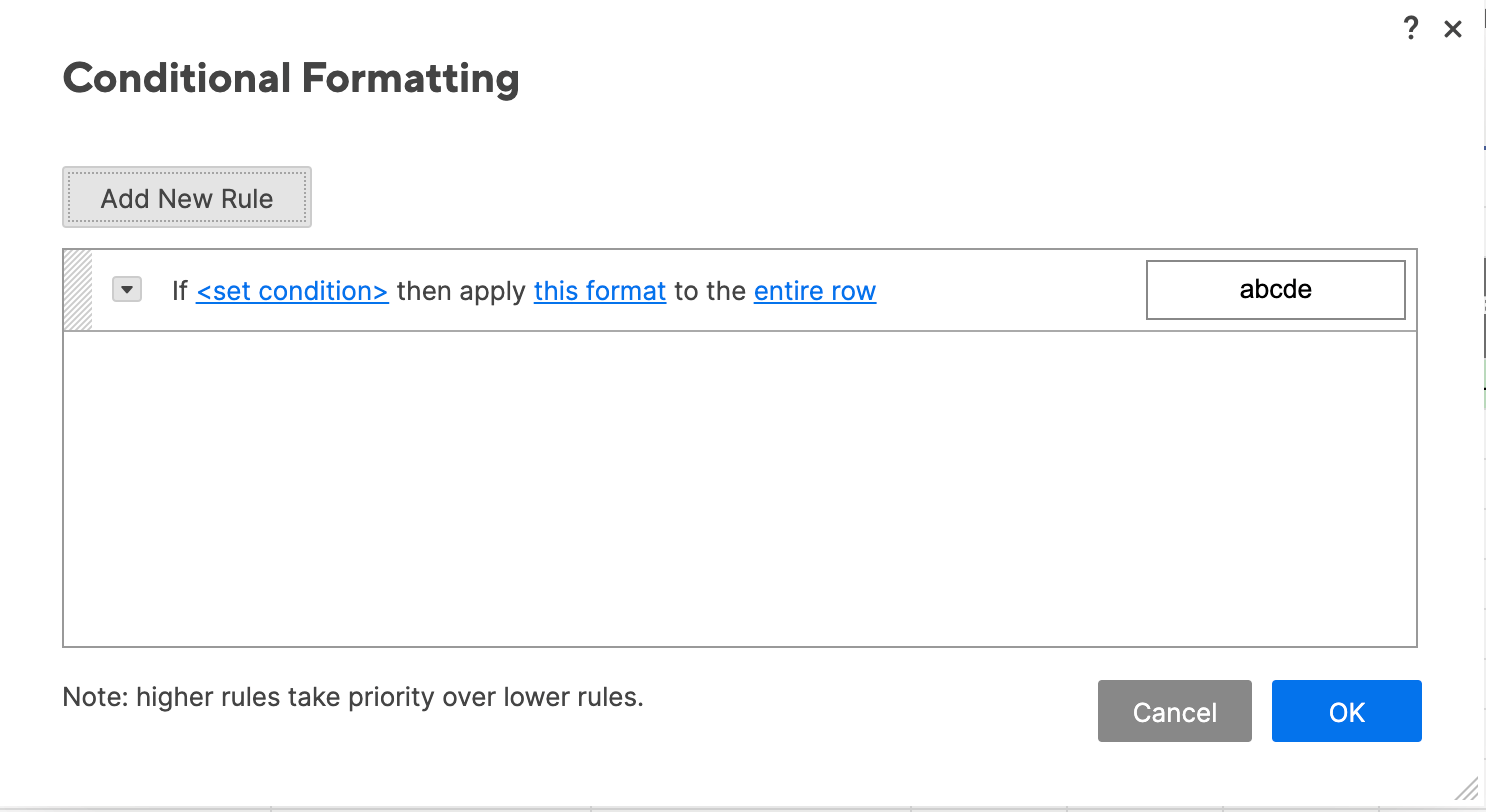
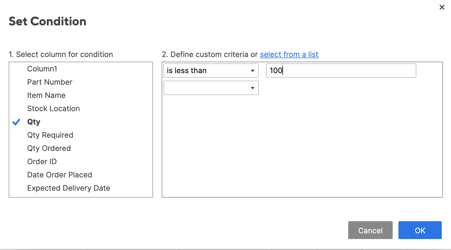
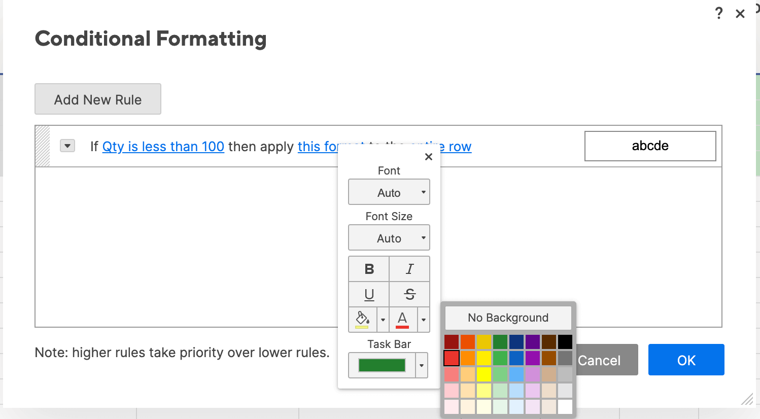
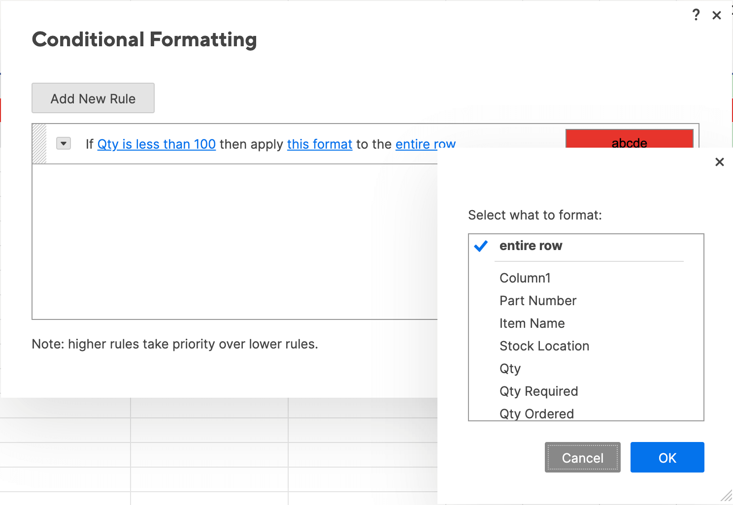
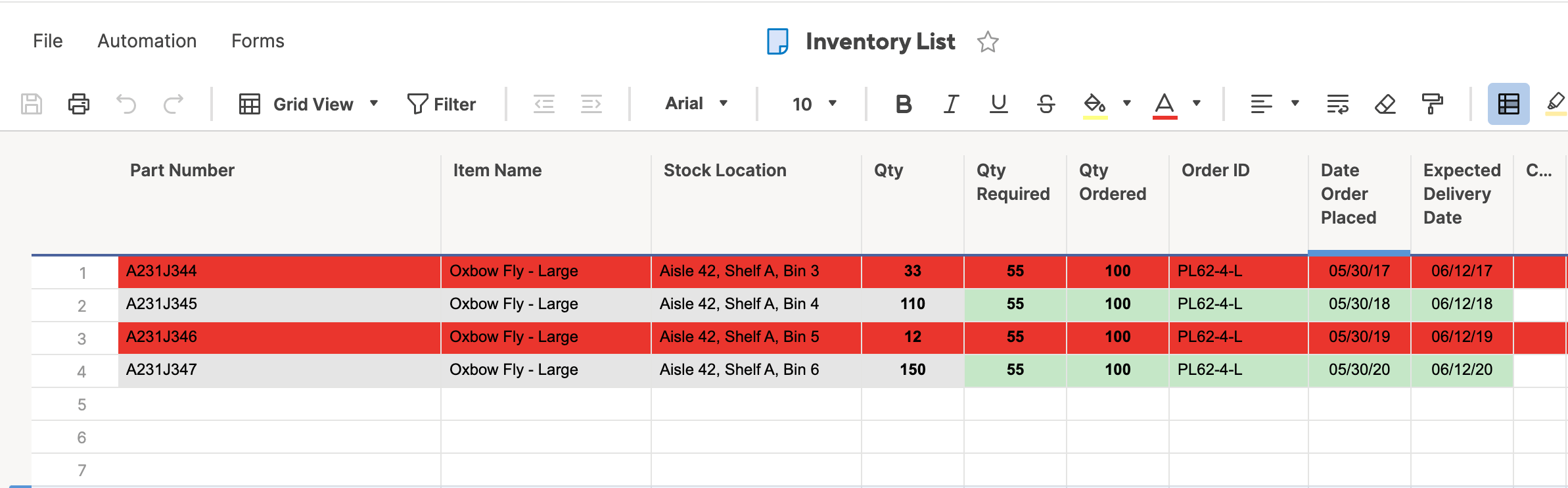
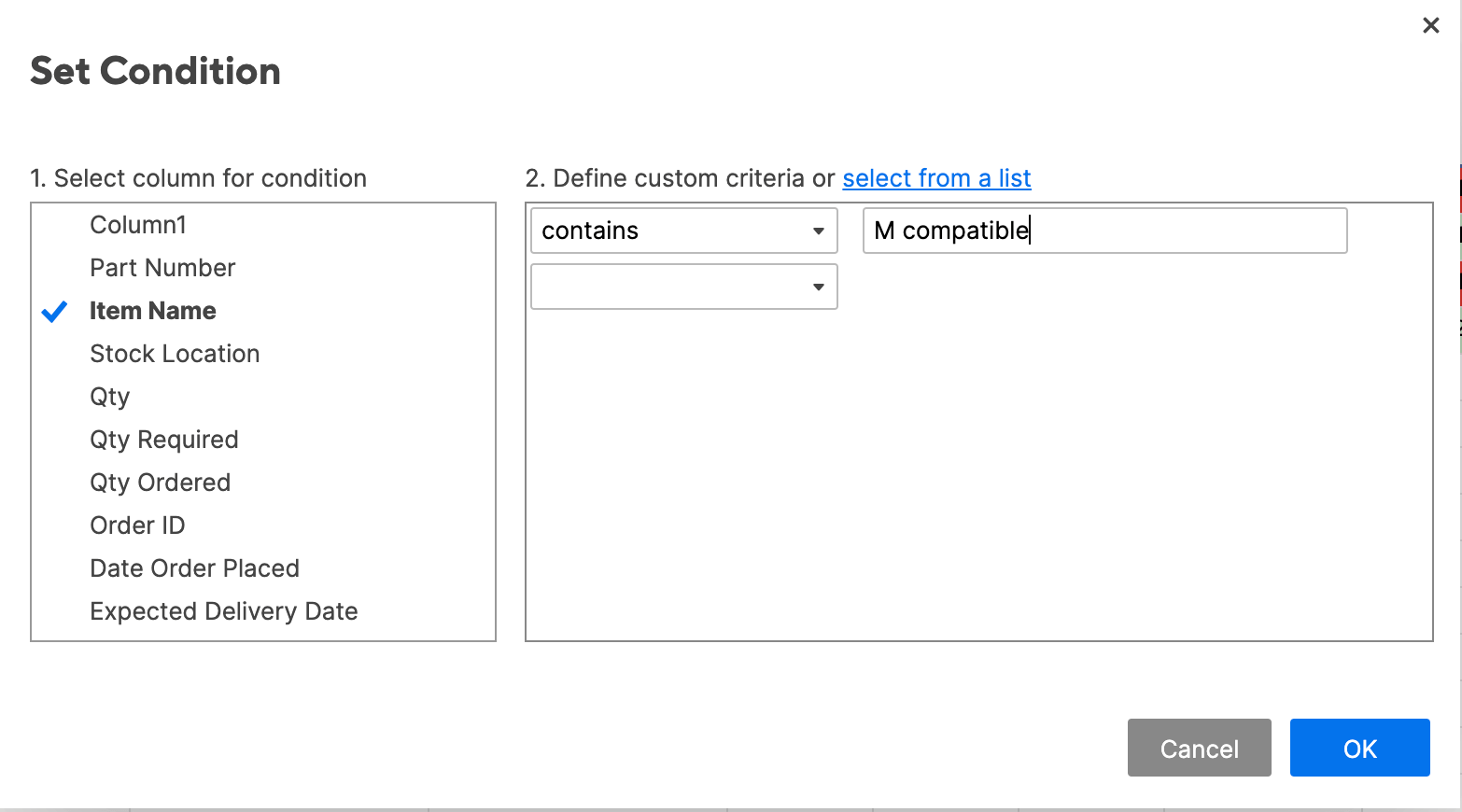
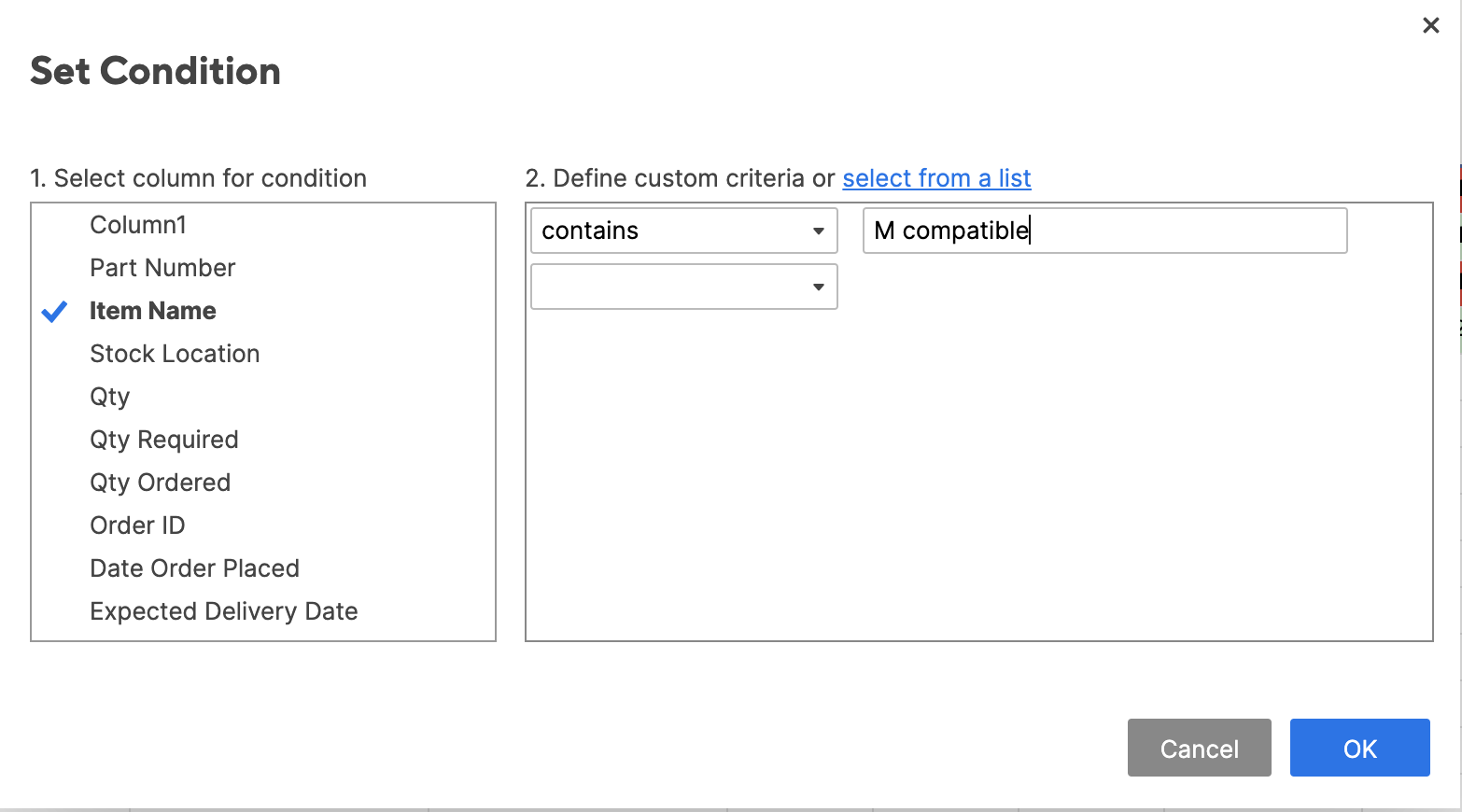
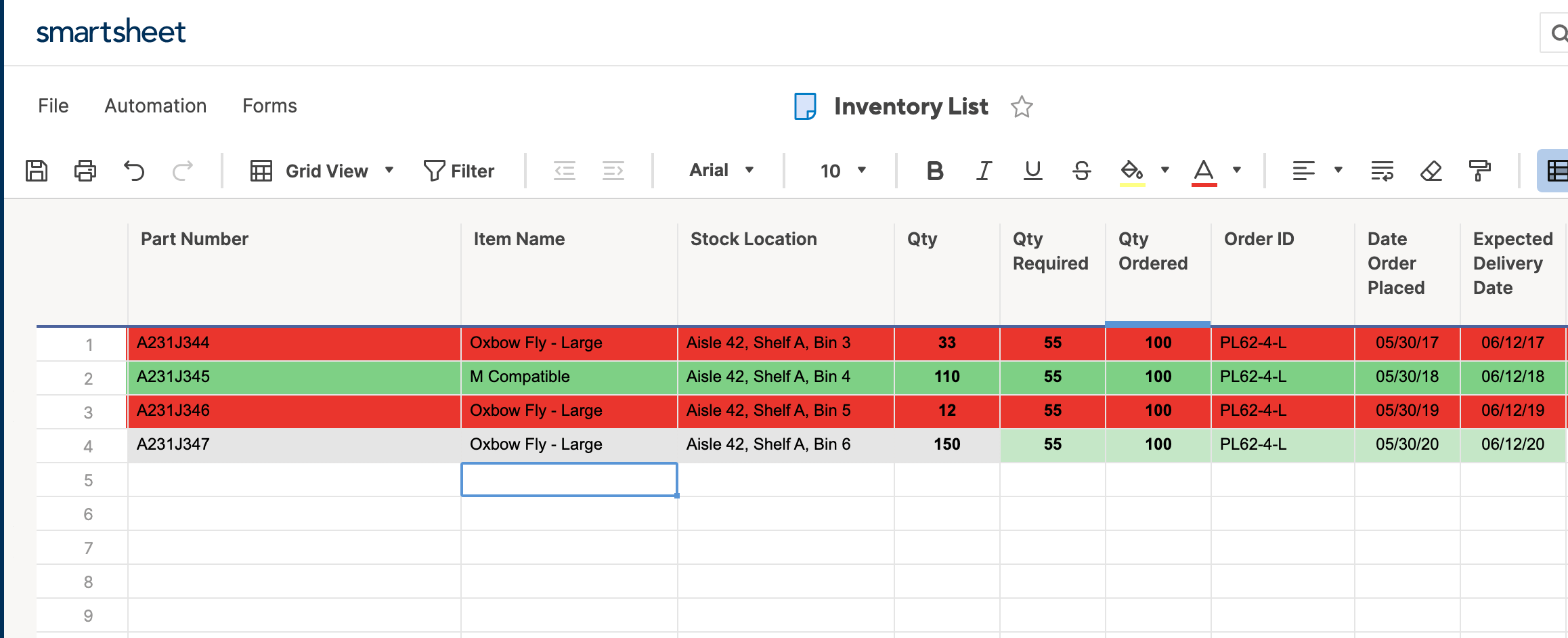
Step 3: Apply Progress Bars (Data Bars)

In place of Excel’s Data Bars preset, you can create Progress Bars in Smartsheet. Progress Bars are a symbol that you can apply to cells to show and compare the level of completeness. In this example, we’ll apply progress bars to denote current inventory levels (from zero to 100 percent).

To create Progress Bars in Smartsheet, you first need to create a new Symbols column. Cells in a Symbols column will only hold special characters, such as progress bars.
To create a new column, right-click the Qty. column and click Insert Column Right.
A box will open. We’ll name this column Inventory Level, and select Symbols… from the list of column-types. In the right-hand field, scroll down and select the progress bar icon. Click OK.
Click into cells in the new Inventory Level column and select the appropriate level of inventory: Empty, Quarter, Half, Three Quarter, or Full. This progress bar relates the current level (from the Qty. column) to level you need.
Here’s what your sheet will look like when all progress bars are filled in.

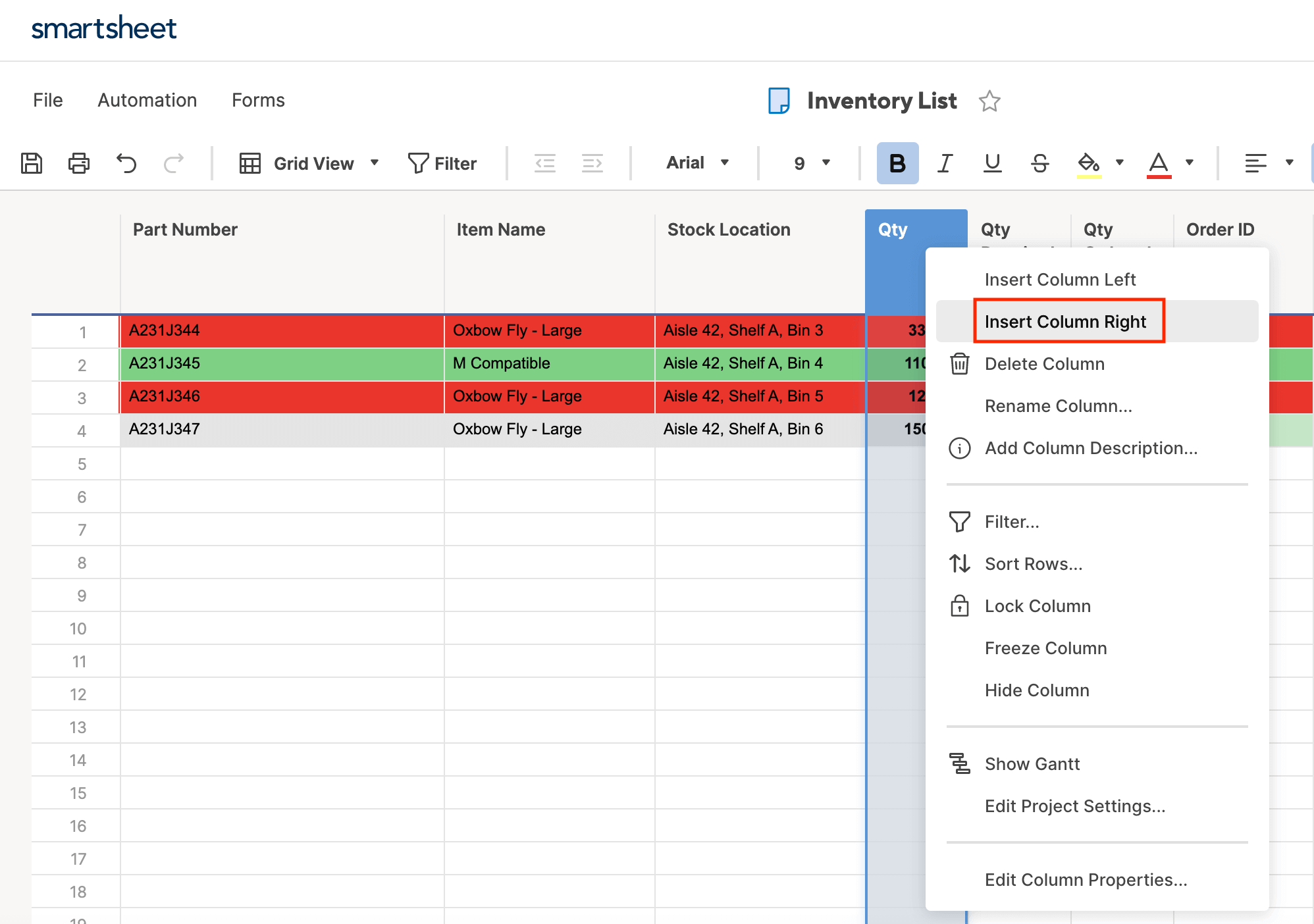
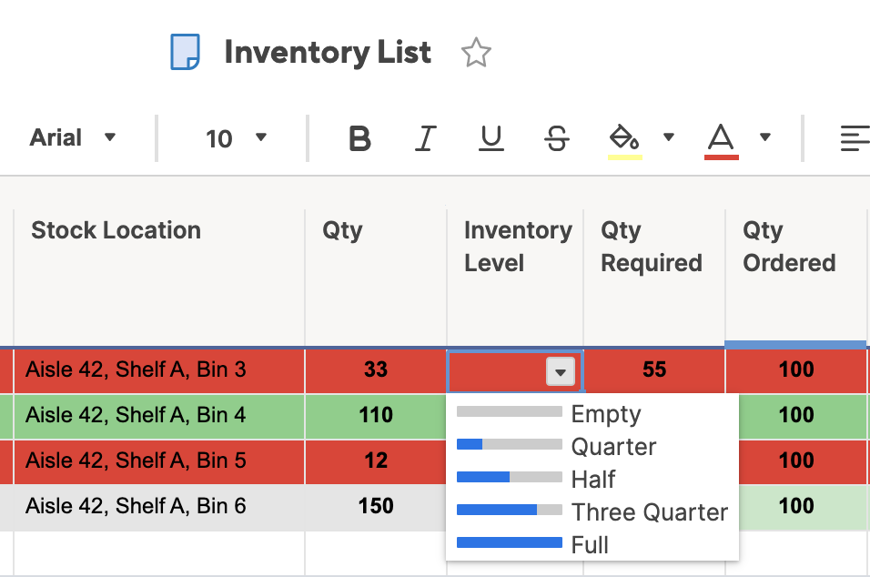
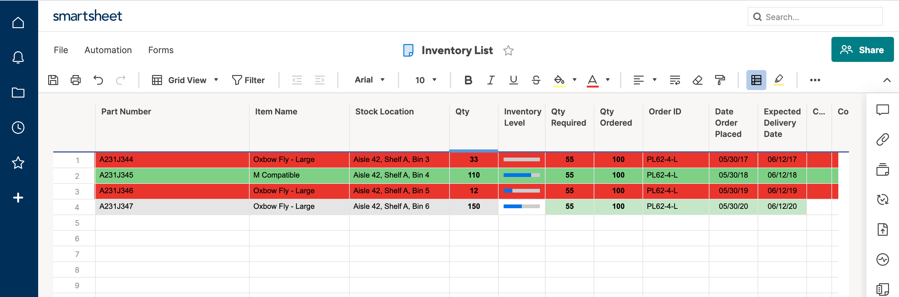
Tip: You can also type Empty, Quarter, Half, Three Quarter, or Full into each cell, and Smartsheet will autofill with the appropriate progress bar.

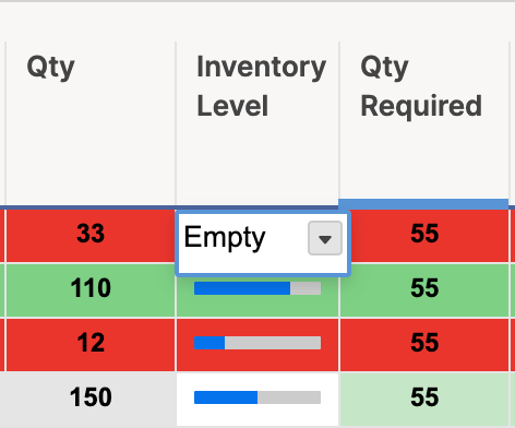
Tip: You can also automate progress bars by using an if-then formula in Smartsheet. For more information on how to do this, check out this resource on symbol formulas.

Step 4: Apply Icon Sets

To apply icon sets in Smartsheet with conditional formatting, you’ll have to use formulas (we’ll get into that in the “Advanced” section). Instead, you can add informative icons to your data by creating a special Symbols column.

Right-click the Qty. column and click Insert Column Right.
In the box that opens, type Qty. Status in the name field. Click Symbols from the dropdown menu and choose from the library of available symbols (Flag, Priority, Decision, Status, Direction, and Measure icons). In this example, we’ll choose RYG balls in the Status section. Click OK.
Now, you can update your sheet with the appropriate color status ball by adding conditional formatting as shown above.

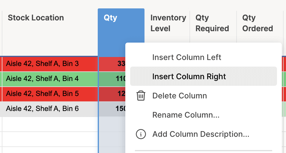
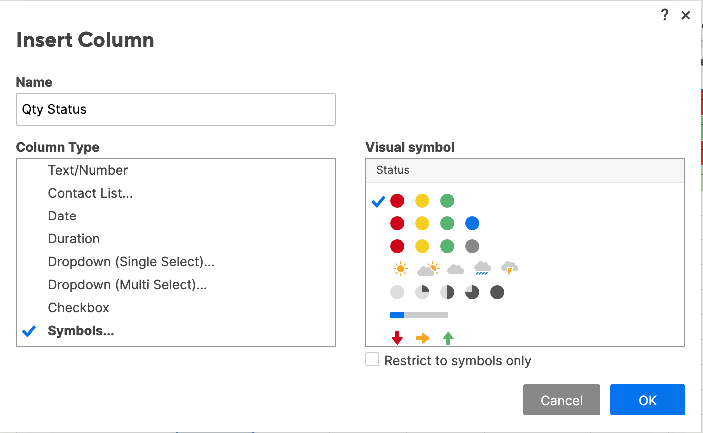
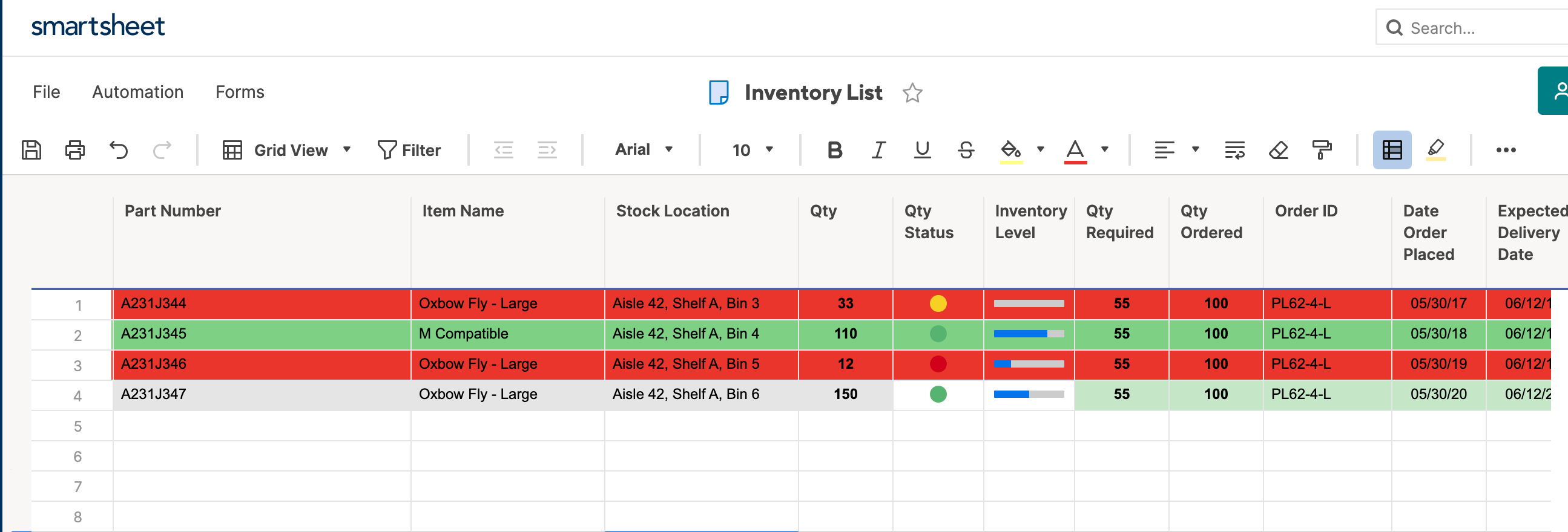
Step 5: Edit and Delete Conditional Formatting Rules

Editing and deleting conditional formatting rules in Smartsheet is extremely easy.

To edit a rule, click the Conditional Formatting icon on the toolbar to open the list of rules. Click the condition you wish to change and edit the information in the box that opens. Click OK.
To delete a rule, click the carrot on the left side of each rule. Click Delete Rule from the dropdown menu. Click OK.

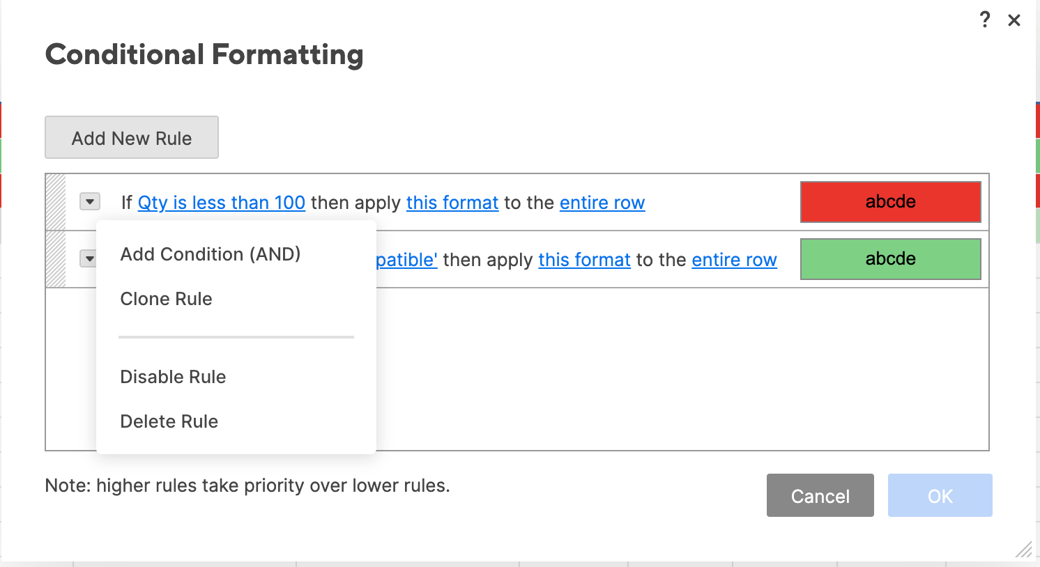
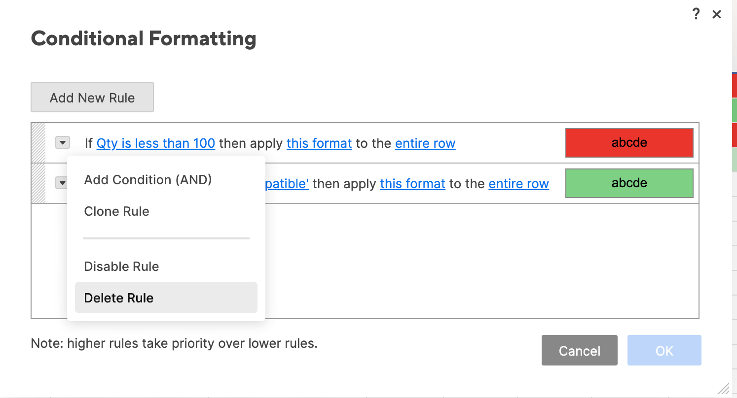
Tip: You can also disable a rule by clicking Disable Rule from the dropdown menu and then clicking OK. This will put the rule on “hold” without deleting it, in case you want to re-enable it later on.

Now you know how to use conditional formatting and other colors and symbols to add formatting to your sheet in Smartsheet. In the following sections, we’ll walk you through more advanced conditional formatting functions in Excel and Smartsheet.

Advanced Conditional Formatting Functions in Excel

Once you have mastered the basics, Excel includes some additional advanced conditional formatting functions. We’ll guide you through applying stop-if-true rules, using the AND formula, setting rule hierarchies and precedence, and other unique situational formatting conditions below.

Step 1: Create a New Rule and Apply Stop if true Rule

In some instances, you might want to stop a certain condition, without deleting the entire rule. The Stop if true rule in Excel enables you to do so.

In our example, we applied an icon set of three directional arrows to the Purchase price column to indicate low, medium, and high price ranges. However, we might actually only want to call attention to the lowest cost items, as three icons can clutter the sheet (and provide more information than actually needed).
First, create a separate condition on this column. Click the Purchase price column to select these values.
Click Conditional Formatting > Manage Rules… to open the Manage Rules box. Keep the default Show formatting rules for: Current Selection from the dropdown menu, because we are only adjusting the rule on this column.
Click the + in the bottom left corner to create a new rule. A new box opens where you can assign conditions to the new rule.
From the Style menu, select Classic.
Instead of applying a different icon to bottom, middle, and top price ranges (as we currently have), we only want to show the bottom 50 percent. So, select Top from the left dropdown menu, type 50 in the middle field, and check the Percent box.
To apply color formatting, Select Custom format from the Format with dropdown menu, and a new formatting box opens. Click the Fill tab, and click No Color.
Next, click the Font tab, and select black text. Click OK.
Click OK again in the original New Formatting Rule box.
You’ll return to the Manage Rules box, where you now have two rules applied to the Purchase price column. Click the Stop if true box to the right of the new rule you just created. Click OK.
Your sheet will now only show the icon sets for the items with a purchase price in the bottom 50 percent.

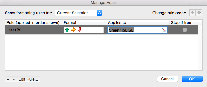
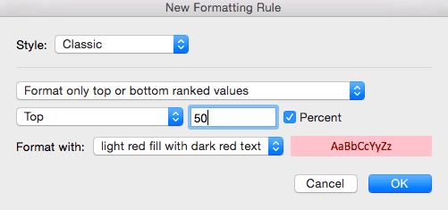
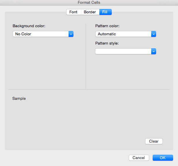
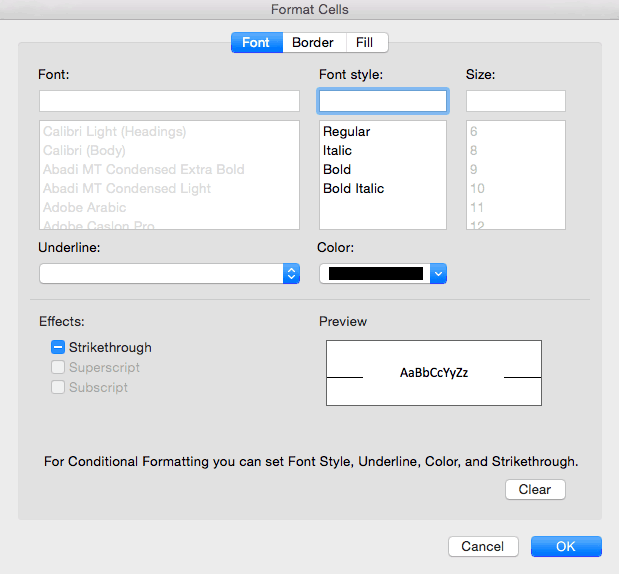
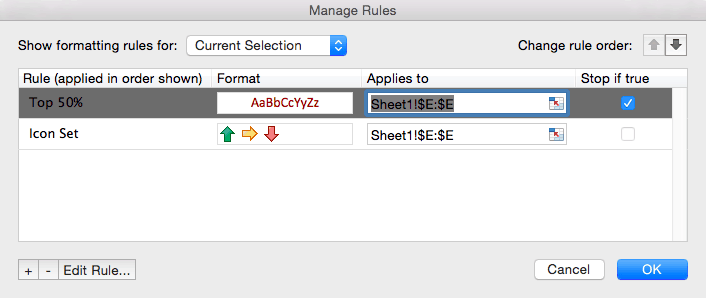
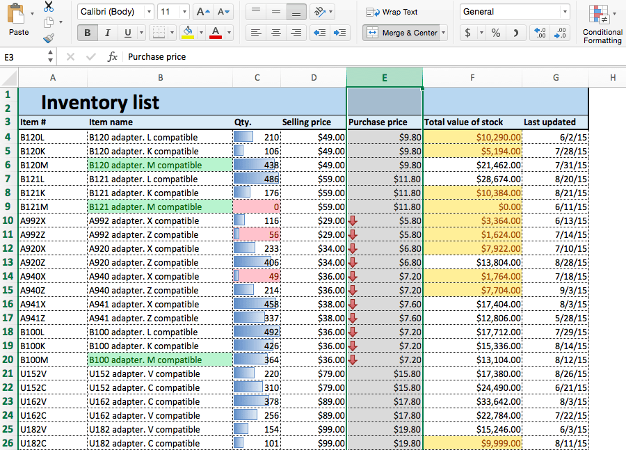
Step 2: Apply Multiple Conditions to a Rule with AND Formula

Adding Excel’s formulas to your conditional formatting rules is one way to elevate your logical rules. The AND formula is one of the most popular, easy-to-use formulas. It lets you add multiple conditions within a single rule, rather than writing out each rule separately. To format cells they must meet both conditions.

We’ll create a new rule to highlight any cell in the Item # column that contains both a B and an L. Click the top of the Item # column to select this range of cells.
Click Conditional Formatting > New Rule.
In the dialogue box, select Classic from the top dropdown list. Select Use a formula to determine which cells to format, since we’re using a formula.
We want to search cells in the Item # column for a B and L, and highlight that cell when both conditions are true. To do this, we’ll use Excel’s ISNUMBER and SEARCH formulas, with the AND formula, to look for the B and L values.
=AND(ISNUMBER(SEARCH(«B»,A1)),ISNUMBER(SEARCH(«L»,A1)))
Click OK. Your sheet will highlight all cells in Item # that meet both of these conditions.

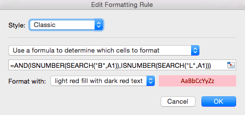
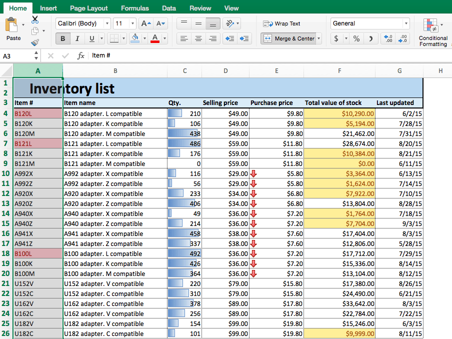
Tip: Understanding the formula:

We use AND at the beginning of the formula to show that both of the following conditions must be met in order to apply the conditional formatting.
The basic syntax of the nested formula is ISNUMBER(SEARCH(“substring”,text)) where “substring” is the character(s) you are looking for, and “text” is the cell(s) you want to search.
We are searching for two separate conditions, so we write the ISNUMBER(SEARCH(“substring”,text)) formula twice, separated by a comma.

This example is just one of hundreds of different formulas you could enter with the AND function. For more information on using Excel formulas with conditional formatting, click here.

Step 3: Conditional Formatting Based on Another Cell

You can also create rules to highlight certain cells based on the value of another cell.

In this example, we’ll create a “quantity threshold” — items with inventory level below this threshold will be considered “at risk.” We already have a rule that highlights cells in the Qty. column under 100. However, that threshold might change over time, depending on manufacturing or selling rates. So, we want to create a highlight rule that is dependent upon a threshold that we set.
To the right of your data, create a box for Quantity Threshold and choose an amount. In this example, we use 200. (Note the cell you type the amount in. Here, it’s I5.)
Create a new rule by clicking Conditional Formatting > New Rule.
In the dialogue box, click Classic and Use a formula to determine which cells to format from the dropdown menus.
In the formula field, type =C4<$I$5 and keep the default formatting. Click OK.
Numbers in the Qty. column that are less than the Quantity Threshold in I5 (200) will now be highlighted.
Now, you’ve created a dynamic rule. This means that as your threshold changes, the rule will still be applied to the Qty. column and the formatting will adjust as appropriate.

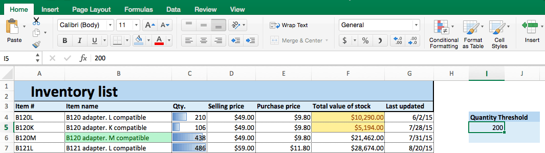
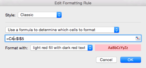
Tip: Understanding the formula:

In this formula, we are simply testing whether or not values in column C are less than the value in I5.
Start with “=C4” to tell Excel where we want to start evaluating values from.
Use ‘$’ symbol around I because it’s an absolute value — we are only evaluating cells in column C against this single cell.

Step 4: Data Validation and Dropdown Lists

While data validation is not technically monitored through conditional formatting rules, you can use it to a similar effect: controlling the formatting of your sheet. You can apply data validation to ensure that any cell-type only allows certain entries (text or numbers only, text length, etc.). In this example, we’ll show you how to create a dropdown list and validate data only from that dropdown list.

We’ll create an additional column of which employee last updated the sheet, and create a dropdown list to choose from. First, click where you want to add the column on the sheet. Create a new column by clicking Insert > Insert Sheet Columns from the ribbon on the Home tab.
We’ll name this column Updated By.
Now we need to make a list of employees, that the dropdown list will later pull from. Create a second sheet (in the same Excel workbook) by clicking the + sign on the tab at the bottom of the spreadsheet, and write a list of employee names in column B.
Select the range of data (all the names) you want to include in your list. Make this list into a table by clicking the Insert tab > Table.
The dialogue box will show the range of data you selected for the table. Click My table has headers, since we began the list with Employees. Click OK.
Now we have to name this list so that Sheet 1 can pull from it. Click Formulas tab > Define Name on the ribbon.
In the dialogue box, type the name of the list. We’ll call it Employees. Double check that the selected range is still correct. Click OK.
Go back to Sheet 1. Now, we have to make the Updated By column into a dropdown list. We’ll use the data validation function to do this.
Select the Updated By column to apply data validation to this range of cells.
Click the Data tab on the ribbon and click Data Validation > Data Validation…
In the dialogue box, choose List from the dropdown menu to restrict data entered in this range to a list. Type =Employees in the Source field, since we’re pulling from the list we just created (in Sheet 2). Click OK.
There is now a dropdown list in the Updated By column. Your sheet will only accept data in this column that comes from the Employees list on Sheet 2.
You can now fill in the column by selecting a name from the dropdown list.

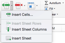
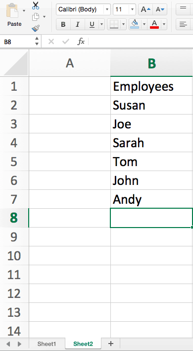
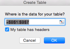
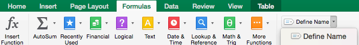
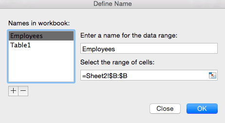
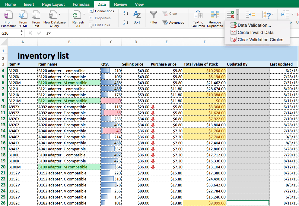
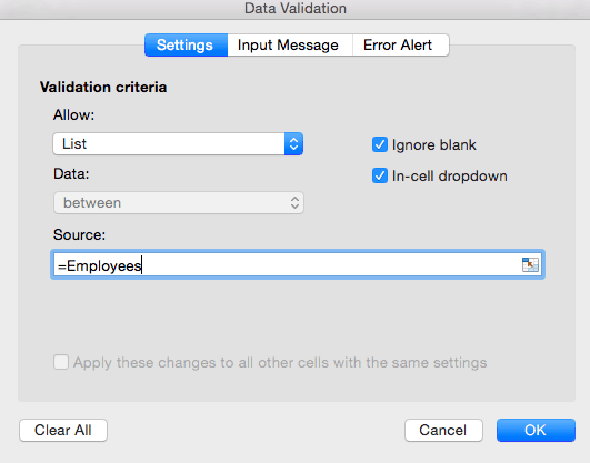
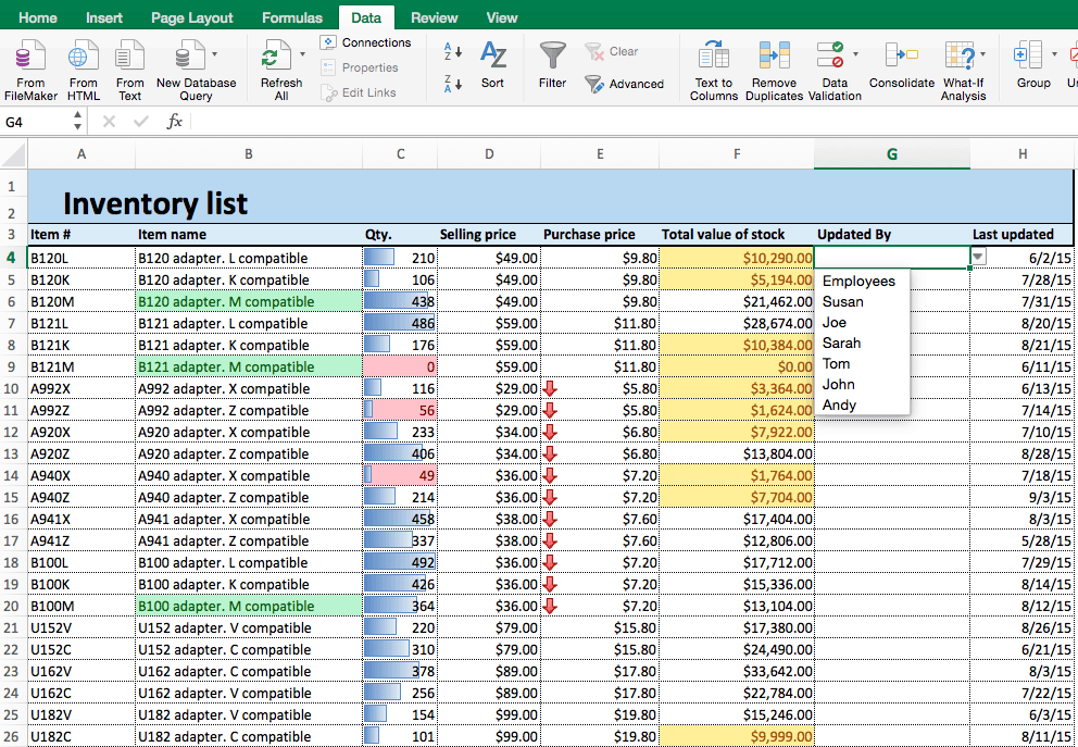
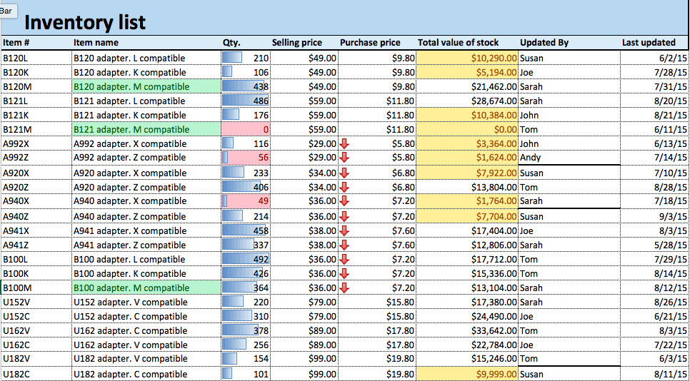
Step 5: Rule Hierarchy and Precedence

As you accumulate conditional formatting rules, watch out for rule hierarchy. Since you can apply multiple conditions to a cell (or row), they occasionally conflict. When this happens, Excel has default precedence rules that may cause one rule to override another, so you can lose your formatting. To combat this, you can change the hierarchy of the rules.

Adjusting rule hierarchy in Excel is straightforward, but you should also understand the logic behind rule precedence:

Newer rules will always assume precedence over older rules. This means that the precedence of your rules will be in the reverse order of how you created them.
When multiple rules evaluate as true to a cell, they may or may not conflict. Applying multiple rules to a cell does not necessarily mean that they will interfere.
Rules don’t conflict if they are changing different things about the cell. For instance, if one rule changes text color and another changes fill color both rules should co-exist in the cell.
Rules conflict when the outcomes are the same. For instance, if one rule changes a font color to green and another changes the font color to blue the newer rule takes precedence.

To adjust rule hierarchy in Excel, follow these steps:

All rule hierarchy is controlled through the Rule Manager in Excel.
From the Home tab, click Conditional Formatting > Manage Rules… to open the Rule Manager.
Select This Sheet from the top dropdown list to pull up all lists applied to the current sheet.
To change the order (hierarchy) of rules, select a rule and click the up and down arrows in the top right corner to move it. Click OK. Remember the rule closest to the top will take precedence.

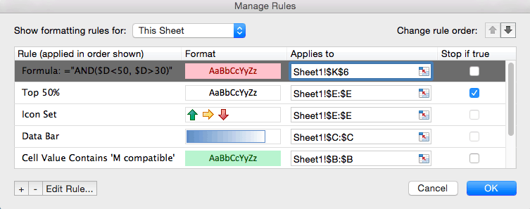
Advanced Conditional Formatting in Smartsheet

Many advanced Excel conditional formatting options are available to Smartsheet users, as well. We’ll teach you how to apply stop-if-true rules, create rules with multiple conditions, create formatting rules based on other cells, and set rule hierarchies and precedence.

Step 1: Add New Rule and Apply Stop If True Function

Adding a new rule in Smartsheet is easy (you already learned how in the “Basic” section). Now, we’ll apply the same “stop if true” logic from Excel in Smartsheet.

Add a new rule by clicking the conditional formatting icon on the toolbar. Click Add New Rule and click Set condition.
For this rule, we want to call attention to the shipment order dates that are after 06/20/30. The easiest way to do this is to apply the same logic as “stop if true” in Excel.
Click Shipment Order Date in the left field to set a condition in this column.
Instead of defining criteria (as we have been doing), click select from a list. The list of values in the Shipment Order Date column appear.
Click 06/20/30. Then, because we want to highlight all the dates that are not this date, check the Apply format when this condition is NOT met box. (This functions just like the “stop if true” box in Excel.) Click OK.
Click this format and apply whatever format you want. We’ll make the text bold.
Click entire row and select the Shipment Order Date column. Click OK.
Now, all dates other than 07/01/15 will be bolded in the Shipment Order Date column.

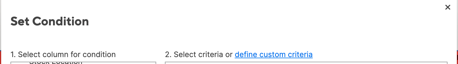
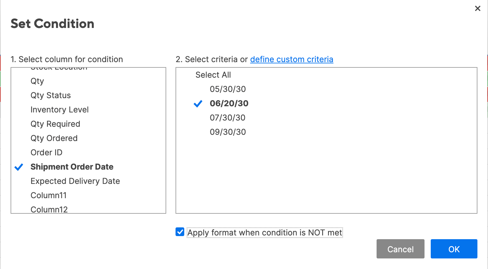
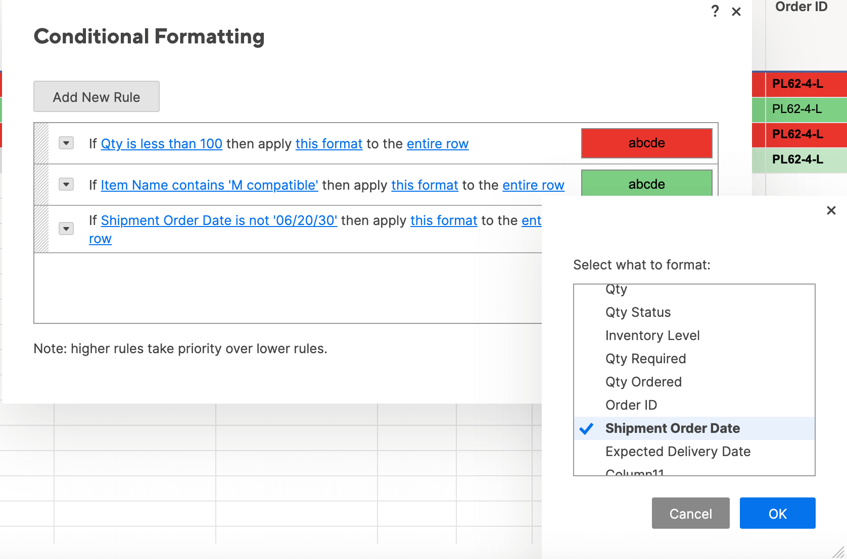
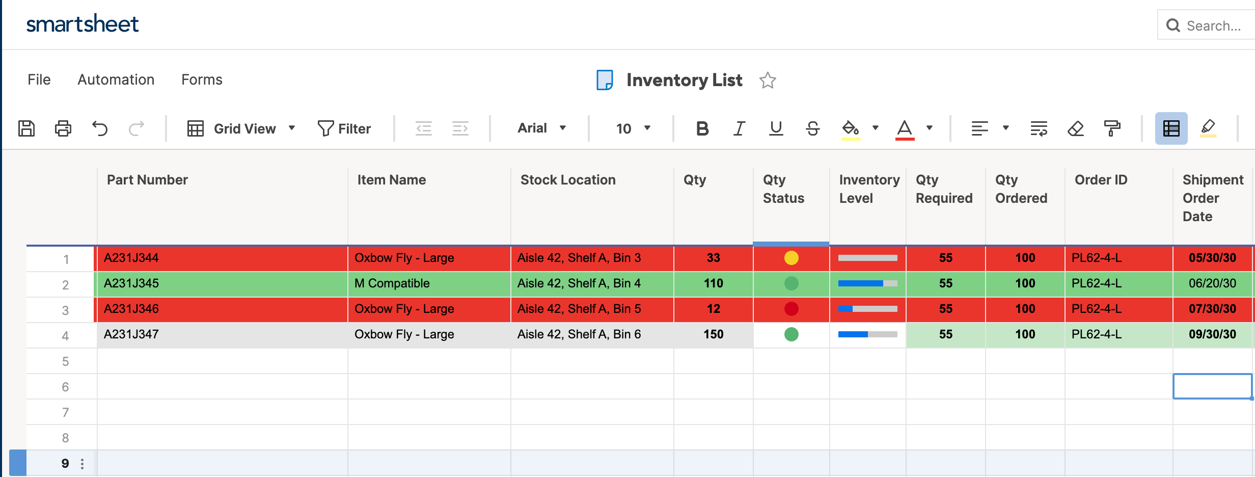
Step 2: Add Multiple Conditions to a Rule

Just like in Excel, you can use Smartsheet’s built-in formulas when creating conditional formatting rules. However, Smartsheet makes it easy to perform some of the simple functions that basic Excel formulas provide, so you don’t have to worry about remembering complicated formula syntax. To perform the AND function, you can simply click to add multiple conditions to any conditional formatting rule.

Click the conditional formatting icon on the toolbar and click Add New Rule.
Click set condition. We want to highlight cells in the Item # list that contain both a ‘B’ and an ‘L.’ Click Item # from the dropdown list on the left.
For the conditions, select contains and type B. Click into the second prompted condition and type L to create the second condition. (This will perform the AND function.) Click OK.
Apply the formatting to your rule. We’ll use a yellow fill.
Change entire row to Item #. Click OK.
Your sheet will now highlight those values in Item # that contain both a B and an L.

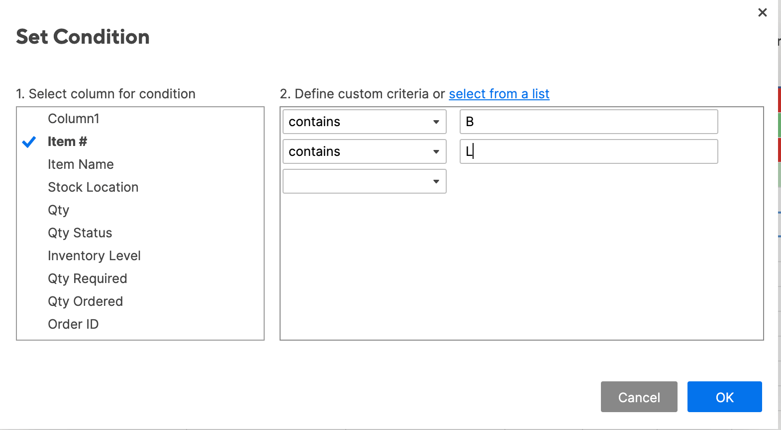
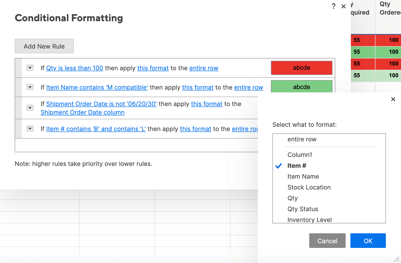
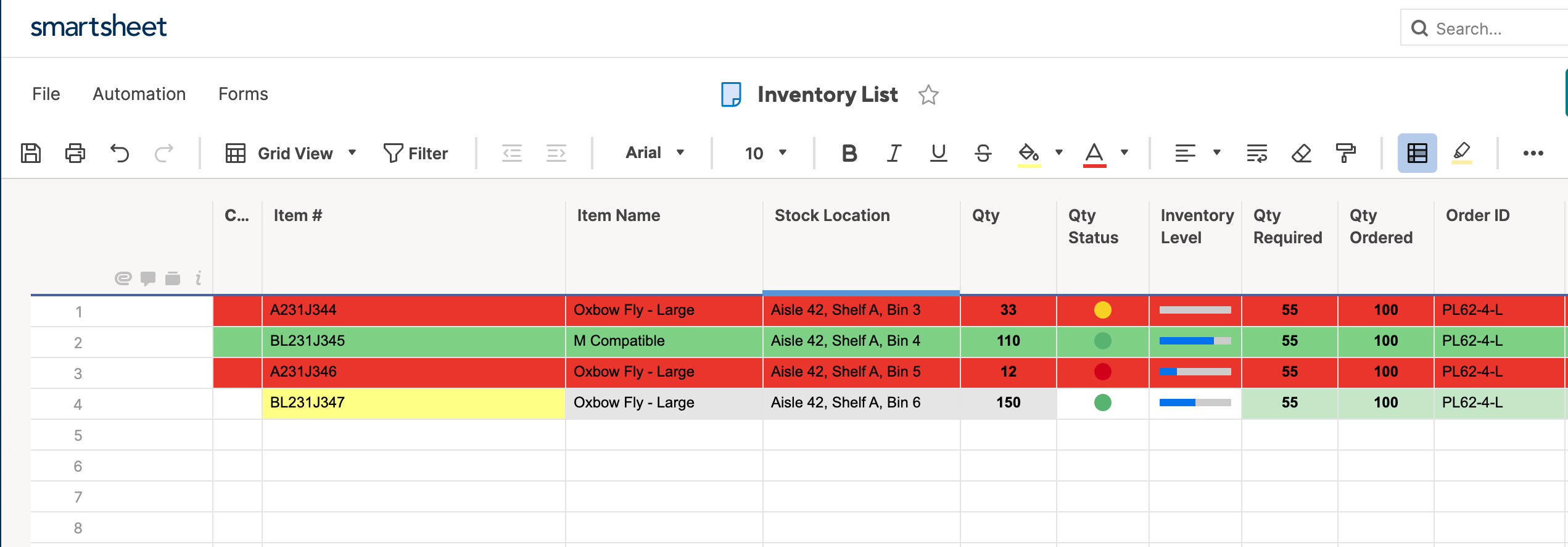
You can still use formulas with conditional formatting, if you’d like. For an introduction on how to use formulas, check out this resource.

Step 3: Conditional Formatting Based on Another Cell

Smartsheet also makes it easy to apply conditional formatting based on another cell. Instead of using complicated formulas to reference different cells, you can simply control which cells to pull from and format with a few clicks.

In this example, we want to highlight the Item Name column if the status bar is red, to call attention to at-risk items. To do this, we’ll create a rule that pulls from the Qty. Status column, but applies formatting to the Item Name column.
Click the conditional formatting icon on the toolbar and click Add New Rule > set condition.
Click Qty. Status from the drop down list and click Red. Click OK.
Apply a light red paint fill to format with.
Click entire row and select Item name. This will apply formatting to cells in the Item name column, even though we’re pulling information from the Qty. Status column.
Click your new rule and drag it to the top of your rules list. Since we have multiple highlighting rules, this will ensure that this rule takes precedence over others.
Cells in Item Name will now be highlighted if the Qty. Status ball is red.

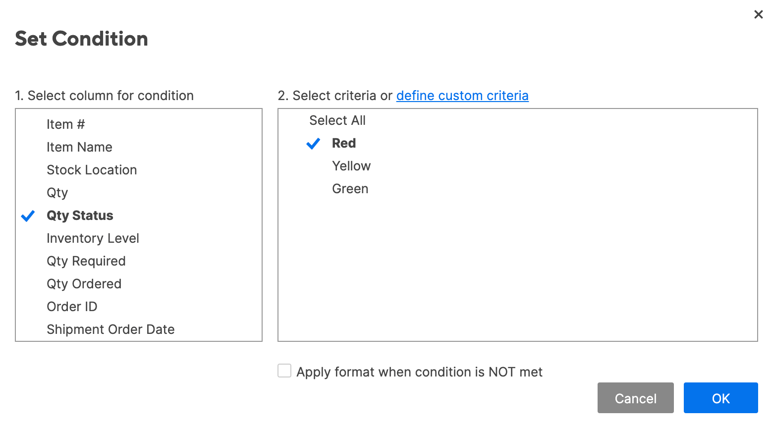
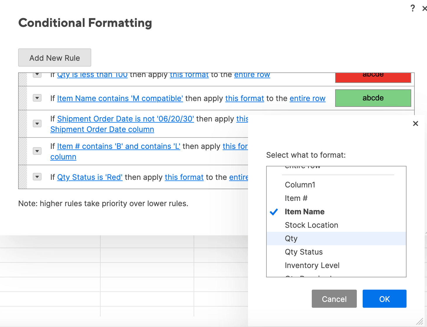
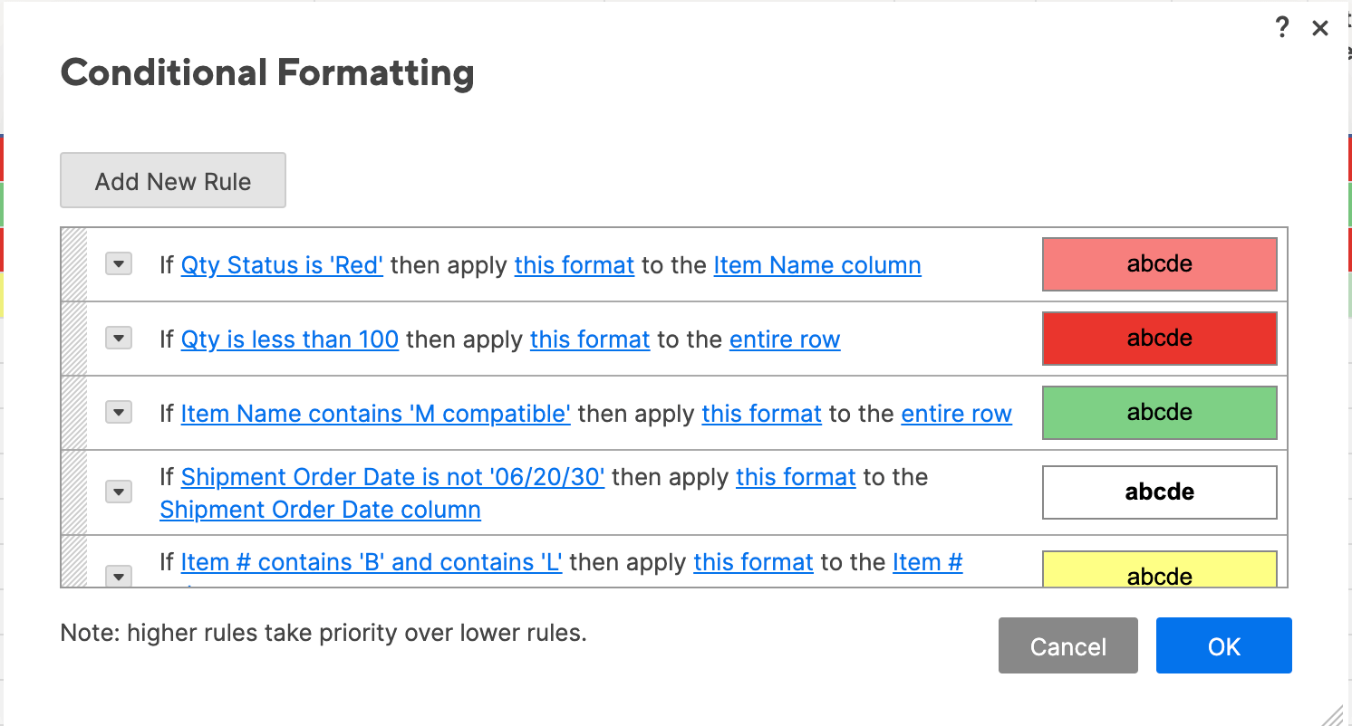
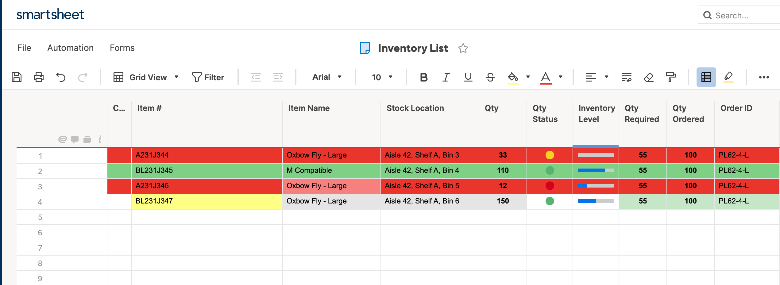
Tip: To eliminate visual redundancy, you can hide the Qty. Status column in your sheet. Simply right-click the column and click Hide column. Your sheet will retain its formatting based on that column, but it will look cleaner.

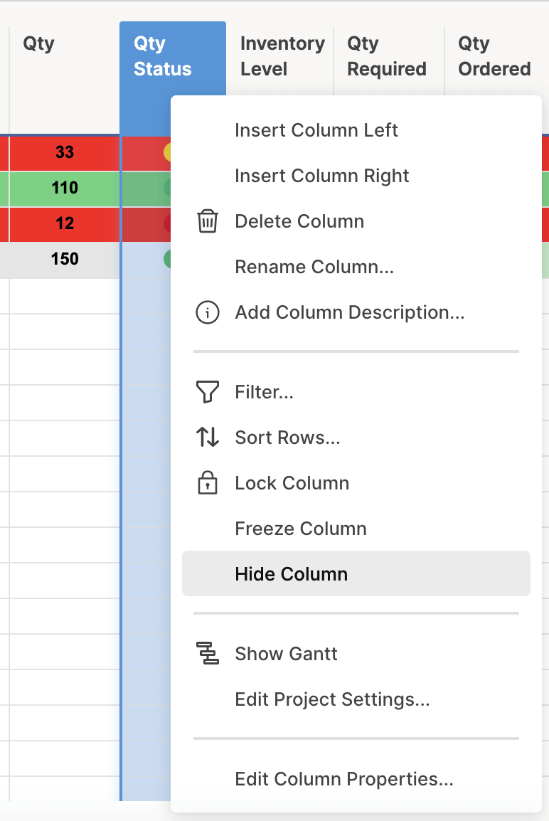
Step 4: Rule Hierarchy and Precedence

Managing rule hierarchy is quite simple in Smartsheet. The rules also interact the same way as Excel (you can apply multiple rules to a single cell, but only one will show up if there’s a conflict). However, the default precedence is a little different:

Click on the conditional formatting icon to bring up the rules.
In Smartsheet, rules higher on this list have precedence. So, the rules have descending hierarchy from the top to bottom of the list.
To change hierarchy, simply click on a rule and drag it up or down.

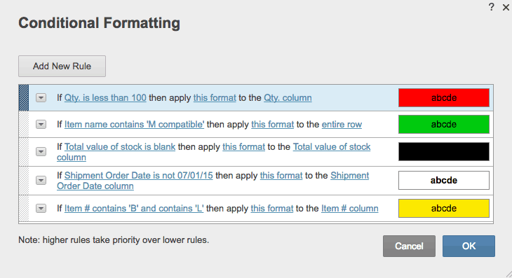
Frequently Asked Questions About Conditional Formatting

The most commonly asked questions about conditional formatting include queries about who can make changes, where to learn about using formulas, and how to copy conditional formatting rules between sheets. We’ve answered these and other frequently asked questions below:

Will conditional formatting change the values in my cells?

No. Conditional formatting only applies formatting to your cells. However, you can use conditional formatting to manipulate the values in your cells by using formulas, or by creating rules that change the value of a cell based on another cell.

Can anyone change or apply conditional formatting to the spreadsheets?

Only one person can update conditional formatting rules in Excel at a time. In Smartsheet, any collaborator with Admin permissions can create or edit conditional formatting, but editors and viewers cannot. Click the Sharing button to adjust permissions.

Does the Office 365 (cloud) version of Excel support conditional formatting?

Users can only view conditional formatting in the cloud version of Excel. To add or edit rules, download the Office 365 desktop version. Be careful of version control issues when working with Office 365.

I’m not comfortable using Excel formulas. Where can I learn more?

Here is a list of common questions for using Excel formulas with conditional formatting. For a comprehensive list of all Excel formulas, click here. For help with using formulas with conditional formatting in Smartsheet, check out these tips.

How do I add conditional formatting to a new document in Excel?

To copy conditional formatting to a new workbook or sheet, select the cells you want to copy conditional formatting from, and click the Format Paint icon. Drag your cursor over the column, rows, or document to apply the rules.

Here’s a walkthrough of this function.

Keep Your Team in Sync with Real Time Conditional Formatting in Smartsheet

Empower your people to go above and beyond with a flexible platform designed to match the needs of your team — and adapt as those needs change.

The Smartsheet platform makes it easy to plan, capture, manage, and report on work from anywhere, helping your team be more effective and get more done. Report on key metrics and get real-time visibility into work as it happens with roll-up reports, dashboards, and automated workflows built to keep your team connected and informed.

When teams have clarity into the work getting done, there’s no telling how much more they can accomplish in the same amount of time. Try Smartsheet for free, today.

Источник

Conditional Formatting is one of the most simple yet powerful features in Excel Spreadsheets.

As the name suggests, you can use conditional formatting in Excel when you want to highlight cells that meet a specified condition.

It gives you the ability to quickly add a visual analysis layer over your data set. You can create heat maps, show increasing/decreasing icons, Harvey bubbles, and a lot more using conditional formatting in Excel.

Using Conditional Formatting in Excel (Examples)

In this tutorial, I’ll show you seven amazing examples of using conditional formatting in Excel:

Quickly Identify Duplicates using Conditional Formatting in Excel.
Highlight Cells with Value Greater/Less than a Number in a Dataset.
Highlighting Top/Bottom 10 (or 10%) values in a Dataset.
Highlighting Errors/Blanks using Conditional Formatting in Excel.
Creating Heat Maps using Conditional Formatting in Excel.
Highlight Every Nth Row/Column using Conditional Formatting.
Search and Highlight using Conditional Formatting in Excel.

1. Quickly Identify Duplicates

Conditional formatting in Excel can be used to identify duplicates in a dataset.

Here is how you can do this:

This would instantly highlight all the cells that have a duplicate in the selected data set. Your dataset can be in a single column, multiple columns, or in a non-contiguous range of cells.

See Also: The Ultimate Guide to Find and Remove Duplicates in Excel.

2. Highlight Cells with Value Greater/Less than a Number

You can use conditional formatting in Excel to quickly highlight cells that contain values greater/less than a specified value. For example, highlighting all cells with sales value less than 100 million, or highlighting cells with marks less than the passing threshold.

Here are the steps to do this:

This would instantly highlight all the cells with values greater than 5 in a dataset.Note: If you wish to highlight values greater than equal to 5, you should apply conditional formatting again with the criteria “Equal To”.

The same process can be followed to highlight cells with a value less than a specified values.

3. Highlighting Top/Bottom 10 (or 10%)

Conditional formatting in Excel can quickly identify top 10 items or top 10% from a data set. This could be helpful in situations where you want to quickly see the top candidates by scores or top deal values in the sales data.

Similarly, you can also quickly identify the bottom 10 items or bottom 10% in a dataset.

Here are the steps to do this:

This would instantly highlight the top 10 items in the selected dataset. Note that this works only for cells that have a numeric value in it.

Also, if you have less than 10 cells in the dataset, and you select the options to highlight Top 10 items/Bottom 10 Items, then all the cells would get highlighted.

Here are some examples of how the conditional formatting would work:

4. Highlighting Errors/Blanks

If you work with a lot of numerical data and calculations in Excel, you’d know the importance of identifying and treating cells that have errors or are blank. If these cells are used in further calculations, it could lead to erroneous results.

Conditional Formatting in Excel can help you quickly identify and highlight cells that have errors or are blank.

Suppose we have a dataset as shown below:

This data set has a blank cell (A4) and errors (A5 and A6).

Here are steps to highlight the cells that are empty or have errors in it:

This would instantly highlight all the cells that are either blank or have errors in it.

Note: You don’t need to use the entire range A1:A7 in the formula in conditional formatting. The above-mentioned formula only uses A1. When you apply this formula to the entire range, excel checks one cell at a time and adjusts the reference. For example, when it checks A1, it uses the formula =OR(ISBLANK(A1),ISERROR(A1)). When it checks cell A2, it then uses the formula =OR(ISBLANK(A2),ISERROR(A2)). It automatically adjusts the reference (as these are relative references) depending on which cell is being analyzed. So you need not write a separate formula for each cell. Excel is smart enough to change the cell reference all by itself 🙂

See Also: Using IFERROR and ISERROR to handle errors in excel.

5. Creating Heat Maps

A heat map is a visual representation of data where the color represents the value in a cell. For example, you can create a heat map where a cell with the highest value is colored green and there is a shift towards red color as the value decreases.

Something as shown below:

The above data set has values between 1 and 100. Cells are highlighted based on the value in it. 100 gets the green color, 1 gets the red color.

Here are the steps to create heat maps using conditional formatting in Excel.

Select the data set.
Go to Home –> Conditional Formatting –> Color Scales, and choose one of the color schemes.

As soon as you click on the heatmap icon, it would apply the formatting to the dataset. There are multiple color gradients that you can choose from. If you are not satisfied with the existing color options, you can select more rules and specify the color that you want.

Note: In a similar way, you can also apply Data Bard and Icon sets.

6. Highlight Every Other Row/Column

You may want to highlight alternate rows to increase the readability of the data.

These are called the zebra lines and could be especially helpful if you are printing the data.

Now there are two ways to create these zebra lines. The fastest way is to convert your tabular data into an Excel Table. It automatically applied a color to alternate rows. You can read more about it here.

Another way is using conditional formatting.

Suppose you have a dataset as shown below:

Here are the steps to highlight alternate rows using conditional formatting in Excel.

That’s it! The alternate rows in the data set will get highlighted.

You can use the same technique in many cases. All you need to do is use the relevant formula in the conditional formatting. Here are some examples:

Highlight alternate even rows: =ISEVEN(ROW())
Highlight alternate add rows: =ISODD(ROW())
Highlight every 3rd row: =MOD(ROW(),3)=0

7. Search and Highlight Data using Conditional Formatting

This one is a bit advanced use of conditional formatting. It would make you look like an Excel rockstar.

Suppose you have a dataset as shown below, with Products Name, Sales Rep, and Geography. The idea is to type a string in cell C2, and if it matches with the data in any cell(s), then that should get highlighted. Something as shown below:

Here are the steps to create this Search and Highlight functionality:

That’s it! Now when you enter anything in cell C2 and hit enter, it will highlight all the matching cells.

How does this work?

The formula used in conditional formatting evaluates all the cells in the dataset. Let’s say you enter Japan in cell C2. Now Excel would evaluate the formula for each cell.

The formula would return TRUE for a cell when two conditions are met:

Cell C2 is not empty.
The content of cell C2 exactly matches the content of the cell in the dataset.

Hence, all the cells that contain the text Japan get highlighted.

Download the Example File

You can use the same logic, to create variations such as:

Highlight the entire row instead of a cell.
Highlight even when there is a partial match.
Highlight the cells/rows as you type (dynamic) [You are going to love this trick :)].

How to Remove Conditional Formatting in Excel

Once applied, conditional formatting remains in place unless you remove it manually. As a best practice, keep the conditional formatting applied only to those cells where you need it.

Since it’s volatile, it may lead to a slow Excel workbook.

To remove conditional formatting:

Select the cells from which you want to remove conditional formatting.
Go to Home –> Conditional Formatting –> Clear Rules –> Clear Rules from Selected Cells.
- If you want to remove conditional formatting from the entire worksheet, select Clear Rules from Entire Sheet.

Important things to know about Conditional Formatting in Excel

Conditional formatting in volatile. It can lead to a slow workbook. Use it only when needed.
When you copy paste cells that contain conditional formatting, conditional formatting also gets copied.
If you apply multiple rules on the same set of cells, all rules remain active. In the case of any overlap, the rule applied last is given preference. You can, however, change the order by changing the order from the Manage Rules dialogue box.

You May Also Like the Following Excel Tutorials:

The Right Way to Apply Conditional Formatting in Pivot Table
Find and Remove Duplicates in Excel
The Ultimate Guide to Using Conditional Formatting in Google Sheets
How to Highlight Weekend Dates in Excel?

Источник

Conditional formatting is a fantastic way to quickly visualize data in a spreadsheet. With conditional formatting, you can do things like highlight dates in the next 30 days, flag data entry problems, highlight rows that contain top customers, show duplicates, and more.

Excel ships with a large number of «presets» that make it easy to create new rules without formulas. However, you can also create rules with your own custom formulas. By using your own formula, you take over the condition that triggers a rule and can apply exactly the logic you need. Formulas give you maximum power and flexibility.

For example, using the «Equal to» preset, it’s easy to highlight cells equal to «apple».

But what if you want to highlight cells equal to «apple» or «kiwi» or «lime»? Sure, you can create a rule for each value, but that’s a lot of trouble. Instead, you can simply use one rule based on a formula with the OR function:

Here’s the result of the rule applied to the range B4:F8 in this spreadsheet:

Here’s the exact formula used:

=OR(B4="apple",B4="kiwi",B4="lime")

Quick start

You can create a formula-based conditional formatting rule in four easy steps:

1. Select the cells you want to format.

2. Create a conditional formatting rule, and select the Formula option

3. Enter a formula that returns TRUE or FALSE.

4. Set formatting options and save the rule.

The ISODD function only returns TRUE for odd numbers, triggering the rule:

Video: How to apply conditional formatting with a formula

Formula logic

Formulas that apply conditional formatting must return TRUE or FALSE, or numeric equivalents. Here are some examples:

=ISODD(A1)
=ISNUMBER(A1)
=A1>100
=AND(A1>100,B1<50)
=OR(F1="MN",F1="WI")

The above formulas all return TRUE or FALSE, so they work perfectly as a trigger for conditional formatting.

When conditional formatting is applied to a range of cells, enter cell references with respect to the first row and column in the selection (i.e. the upper-left cell). The trick to understanding how conditional formatting formulas work is to visualize the same formula being applied to each cell in the selection, with cell references updated as usual. Imagine that you entered the formula in the upper-left cell of the selection, and then copied the formula across the entire selection. If you struggle with this, see the section on Dummy Formulas below.

Formula Examples

Below are examples of custom formulas you can use to apply conditional formatting. Some of these examples can be created using Excel’s built-in presets for highlighting cells, but custom formulas can go far beyond presets, as you can see below.

Highlight orders from Texas

To highlight rows that represent orders from Texas (abbreviated TX), use a formula that locks the reference to column F:

=$F5="TX"

For more details, see this article: Highlight rows with conditional formatting.

Video: How to highlight rows with conditional formatting

Highlight dates in the next 30 days

To highlight dates occurring in the next 30 days, we need a formula that (1) makes sure dates are in the future and (2) makes sure dates are 30 days or less from today. One way to do this is to use the AND function together with the NOW function like this:

=AND(B4>NOW(),B4<=(NOW()+30))

With a current date of August 18, 2016, the conditional formatting highlights dates as follows:

The NOW function returns the current date and time. For details about how this formula, works, see this article: Highlight dates in the next N days.

Highlight column differences

Given two columns that contain similar information, you can use conditional formatting to spot subtle differences. The formula used to trigger the formatting below is:

=$B4<>$C4

See also: a version of this formula that uses the EXACT function to do a case-sensitive comparison.

Highlight missing values

To highlight values in one list that are missing from another, you can use a formula based on the COUNTIF function:

=COUNTIF(list,B5)=0

This formula simply checks each value in List A against values in the named range «list» (D5:D10). When the count is zero, the formula returns TRUE and triggers the rule, which highlights values in List A that are missing from List B.

Video: How to find missing values with COUNTIF

Highlight properties with 3+ bedrooms under $350k

To find properties in this list that have at least 3 bedrooms but are less than $300,000, you can use a formula based on the AND function:

=AND($C5<350000,$D5>=3)

The dollar signs ($) lock the reference to columns C and D, and the AND function is used to make sure both conditions are TRUE. In rows where the AND function returns TRUE, the conditional formatting is applied:

Highlight top values (dynamic example)

Although Excel has presets for «top values», this example shows how to do the same thing with a formula, and how formulas can be more flexible. By using a formula, we can make the worksheet interactive — when the value in F2 is updated, the rule instantly responds and highlights new values.

The formula used for this rule is:

=B4>=LARGE(data,input)

Where «data» is the named range B4:G11, and «input» is the named range F2. This page has details and a full explanation.

Gantt charts

Believe it or not, you can even use formulas to create simple Gantt charts with conditional formatting like this:

This worksheet uses two rules, one for the bars, and one for the weekend shading:

=AND(D$4>=$B5,D$4<=$C5) // bars
=WEEKDAY(D$4,2)>5 // weekends

This article explains the formula for bars, and this article explains the formula for weekend shading.

Simple search box

One cool trick you can do with conditional formatting is to build a simple search box. In this example, a rule highlights cells in column B that contain text typed in cell F2:

The formula used is:

=ISNUMBER(SEARCH($F$2,B2))

For more details and a full explanation, see:

Article: How to highlight cells that contain specific text
Article: How to highlight rows that contain specific text
Video: How to build a search box to highlight data

Troubleshooting

If you can’t get your conditional formatting rules to fire correctly, there’s most likely a problem with your formula. First, make sure you started the formula with an equals sign (=). If you forget this step, Excel will silently convert your entire formula to text, rendering it useless. To fix, just remove the double quotes Excel added at either side and make sure the formula begins with equals (=).

If your formula is entered correctly but is not triggering the rule, you may have to dig a little deeper. Normally, you can use the F9 key to check results in a formula or use the Evaluate feature to step through a formula. Unfortunately, you can’t use these tools with conditional formatting formulas, but you can use a technique called «dummy formulas».

Dummy Formulas

Dummy formulas are a way to test your conditional formatting formulas directly on the worksheet, so you can see what they’re actually doing. This can be a big time-saver when you’re struggling to get cell references working correctly.

In a nutshell, you enter the same formula across a range of cells that matches the shape of your data. This lets you see the values returned by each formula, and it’s a great way to visualize and understand how formula-based conditional formatting works. For a detailed explanation, see this article.

Video: Test conditional formatting with dummy formulas

Limitations

There are some limitations that come with formula-based conditional formatting:

You can’t apply icons, color scales, or data bars with a custom formula. You are limited to standard cell formatting, including number formats, font, fill color and border options.
You can’t use certain formula constructs like unions, intersections, or array constants for conditional formatting criteria.
You can’t reference other workbooks in a conditional formatting formula.

You can sometimes work around #2 and #3. You may be able to move the logic of the formula into a cell in the worksheet, then refer to that cell in the formula instead. If you are trying to use an array constant, try created a named range instead.

More CF formula resources

More than 30 conditional formatting formulas examples
Video training with practice worksheets

Источник

Let’s pretend you have a spreadsheet with 1,000 rows of data — it would be pretty difficult to spot patterns in the data with the naked eye. Enter conditional formatting.

This powerful tool highlights cells that meet a specific condition or «rule.» In other words, it brings your spreadsheet to life by adding color to patterns and trends.

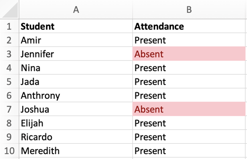
Here, we’ll cover how to apply, edit, and copy and paste conditional formatting.

Conditional Formatting Based on Text

In this example, let’s use conditional formatting to an attendance list to highlight who was absent. The image below is the data set I’ll use to run through this explanation:

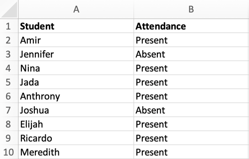
1. First, select the column or row you want to apply conditional formatting to. In this case, we’ll select column B.

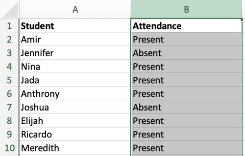
2. To highlight who was absent, navigate to the header toolbar and select Conditional Formatting, as shown in the image below.

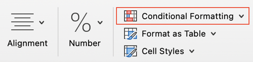
3. When the Conditional Formatting drop-down menu appears, select Highlight Cells Rules, then Equal To.

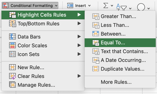
4. In the New Formatting dialog box, change Cell Value to Specific Text. Then, type «Absent» in the text box. Reference the image below:

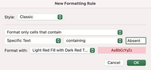
5. From the New Formatting dialog box, we can also choose how we want to format the cells containing the word «Absent.» Check out the options below.

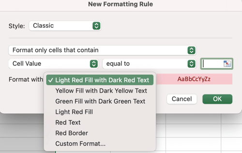
For this example, let’s stick with the default option (Light Red Fill with Dark Red Text).

6. Click OK. Now — thanks to conditional formatting — we can quickly identify which students were absent.

In the next section, we’ll cover how to apply conditional formatting based on another cell in the spreadsheet.

Conditional Formatting Based on Another Cell

In this example, the goal is to highlight the cells that match the drop-down menu in cell E1. The image below is the sample data set I’ll use for this explanation:

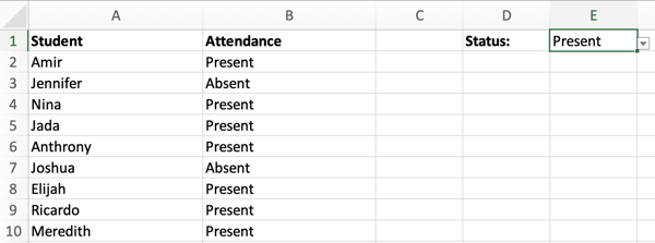
1. First, select column B.

2. Navigate to the header toolbar and select Conditional Formatting. When the Conditional Formatting drop-down menu appears, select Highlight Cells Rules, then Equal To.

3. In the New Formatting dialog box, select Cell Value and Equal To.

In the text box, you can either click your mouse on cell E1 (the cell that contains the drop-down menu), or manually enter the formula =$E$1. See below.

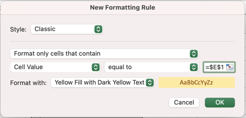
4. As you can see in the image above, we also changed the formatting to Yellow Fill with Dark Yellow Text. However, you can change this option to your preference. Click OK.

5. Now, the cells that match cell E1 are highlighted in yellow. Notice how the highlighted cells change depending on the status:

When the status is Present:

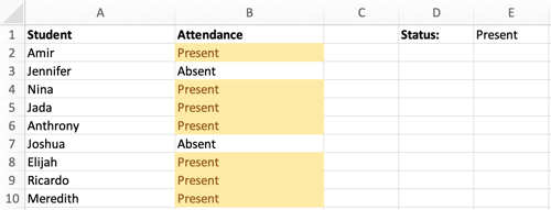
When the status is Absent:

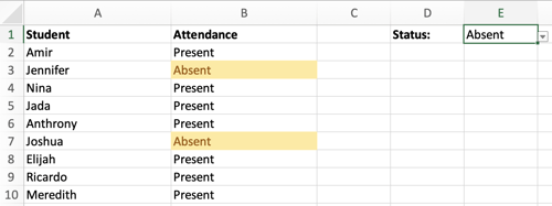
Here’s some good news — conditional formatting is not set in stone, meaning you can edit or delete it later. Here are the steps to do that:

1. Start by selecting the cell (or cell range) that contains a conditional formatting rule.

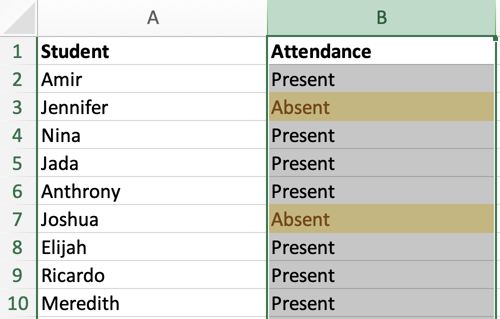
2. Navigate to the header toolbar and select Conditional Formatting, then Manage Rules.

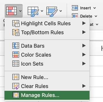
3. The Manage Rules dialog box will list the current rules for your selection. Select the rule you want to edit and click Edit Rule.

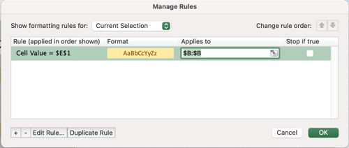
How to Copy Conditional Formatting in Excel

You can easily copy a conditional formatting rule to another cell to (or range of cells) by using one of the following approaches.

1. Simple copy/paste.

The first approach is relatively straightforward. Start by selecting the cell you want to copy and hit the Copy button in the header toolbar — or click Control-C (or Command-C on a Mac).

Then, select the target cell and hit the Paste button in the header toolbar, or click Control-V (or Command-V on a Mac).

2. Format Painter

The second approach uses the tool Format Painter, which is located in the header toolbar. Check out the image below:

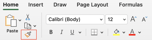
To start, click on the cell you want to copy, then click Format Painter. Your mouse icon will change to a paintbrush. Then, drag the paintbrush to the cell (or range of cells) where you want to paste the format. Lastly, to stop using the paintbrush, press Esc on your keyboard.

Conditional formatting is a powerful way to visualize the data in your spreadsheet. With just a few clicks, you can emphasize important trends or patterns you may have otherwise missed. With the tips in this post, you’ll be able to use Conditional Formatting to its fullest extent.

Источник

Highlight Cells Rules | Clear Rules | Top/Bottom | Conditional Formatting with Formulas

Conditional formatting in Excel enables you to highlight cells with a certain color, depending on the cell’s value.

Highlight Cells Rules

To highlight cells that are greater than a value, execute the following steps.

1. Select the range A1:A10.

2. On the Home tab, in the Styles group, click Conditional Formatting.

3. Click Highlight Cells Rules, Greater Than.

4. Enter the value 80 and select a formatting style.

5. Click OK.

Result. Excel highlights the cells that are greater than 80.

6. Change the value of cell A1 to 81.

Result. Excel changes the format of cell A1 automatically.

Note: you can also use this category (see step 3) to highlight cells that are less than a value, between two values, equal to a value, cells that contain specific text, dates (today, last week, next month, etc.), duplicates or unique values.

Clear Rules

To clear a conditional formatting rule, execute the following steps.

1. Select the range A1:A10.

2. On the Home tab, in the Styles group, click Conditional Formatting.

3. Click Clear Rules, Clear Rules from Selected Cells.

Top/Bottom

To highlight cells that are above average, execute the following steps.

1. Select the range A1:A10.

2. On the Home tab, in the Styles group, click Conditional Formatting.

3. Click Top/Bottom Rules, Above Average.

4. Select a formatting style.

5. Click OK.

Result. Excel calculates the average (42.5) and formats the cells that are above this average.

Note: you can also use this category (see step 3) to highlight the top n items, the top n percent, the bottom n items, the bottom n percent or cells that are below average.

Conditional Formatting with Formulas

Take your Excel skills to the next level and use a formula to determine which cells to format. Formulas that apply conditional formatting must evaluate to TRUE or FALSE.

1. Select the range A1:E5.

2. On the Home tab, in the Styles group, click Conditional Formatting.

3. Click New Rule.

4. Select ‘Use a formula to determine which cells to format’.

5. Enter the formula =ISODD(A1)

6. Select a formatting style and click OK.

Result. Excel highlights all odd numbers.

Explanation: always write the formula for the upper-left cell in the selected range. Excel automatically copies the formula to the other cells. Thus, cell A2 contains the formula =ISODD(A2), cell A3 contains the formula =ISODD(A3), etc.

Here’s another example.

7. Select the range A2:D7.

8. Repeat steps 2-4 above.

9. Enter the formula =$C2=»USA»

10. Select a formatting style and click OK.

Result. Excel highlights all USA orders.

Explanation: we fixed the reference to column C by placing a $ symbol in front of the column letter ($C2). As a result, cell B2, C2 and cell D2 also contain the formula =$C2=»USA», cell A3, B3, C3 and D3 contain the formula =$C3=»USA», etc.

Источник

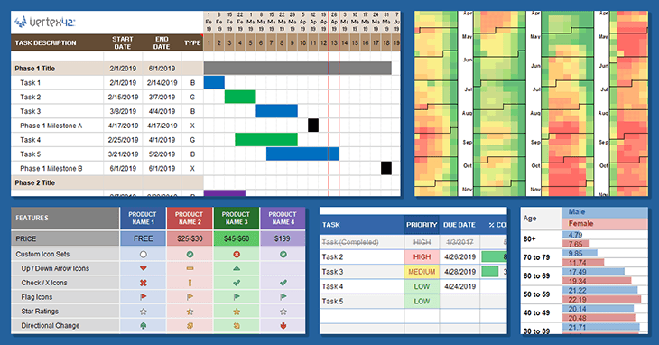
Conditional formatting is one of my favorite features in both Excel and Google Sheets. I love the way it can make a boring hard-to-interpret spreadsheet more interesting and easier to use.

Conditional formatting is mostly used for data analysis, such as adding color scales, highlighting high and low values, identifying duplicates, and marking outliers. Conditional formatting can be also used for graphical interface elements such as progress bars, graying out completed tasks, changing number formats, or displaying a gantt chart.

In this article, I’ll show over 20 different ways that you can use conditional formatting, starting with some basics and presenting some advanced techniques as well. Many of the examples come from templates that you can download and experiment with.

Download the Example File (ConditionalFormatting.xlsx)

This Article (bookmarks):

What is Conditional Formatting?
- How to Highlight Duplicates
- How to add Color Scales
- How to add Data Bars in Excel
- Highlight Overdue Dates
- How to add Icon Sets in Excel
How to View and Edit Conditional Formatting Rules
Rule Order Matters
How to create an In-Cell Progress Bar
How to Highlight Every Other Row
Conditional Formatting Based on Another Cell
How to create a Formula Rule
- How to Highlight an Entire Row
- How to Highlight Based on a Range
- How to Highlight Values NOT in a Range
Create a Gantt Chart
Use Data Bars to Compare Two Groups
Control Scaling by Linking Min/Max to Cells
Change Number Formatting with CF Rules
- Change Date Formats to d/m/yyyy
- Hide Zero Values
- Automatic Indenting
- Display 23K, 23M, 23B Based on Value
- Display Custom Icons
How to Copy Conditional Formatting
Conditional Formatting is Volatile

What is Conditional Formatting?

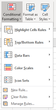
Conditional Formatting in a spreadsheet allows you to change the format of a cell (font color, background color, border, etc.) based on the value in a cell or range of cells, or based on whether a formula rule returns TRUE.

To Apply Conditional Formatting in Excel: First, select the cells you want to format. Then, go to Home > Conditional Formatting and select an option from the built in menu, or click on Manage Rules.

To Apply Conditional Formatting in Google Sheets: First, select the cells you want to format. Then, go to Format > Conditional Formatting and click on «Add another rule» in the side panel.

NOTE Google Sheets currently provides fewer conditional formatting options and controls than Excel (for example, no data bars or icon sets). The focus of this article will be on how to use conditional formatting in Excel, but many of the techniques will apply just as readily to Google Sheets.

Here are a few things you can do with the built-in options in Excel:

1. How to Highlight Duplicates

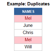
Select your range of cells, then go to Home > Conditional Formatting > Highlight Cells Rules > Duplicates.

After viewing the duplicates, you can decide whether you need to remove them manually or use the built-in tool via Data > Data Tools > Remove Duplicates.

Highlighting duplicates in Google Sheets requires using a custom formula rule such as =COUNTIF(A:A,A1)>1 to highlight the duplicates in column A.

2. How to add Color Scales

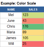
Select your range of cells, then go to Home > Conditional Formatting > Color Scales and pick the color range that makes sense (usually, green=good and red=bad).

Color Scales are very useful for seeing high and low values within a large data set. Color Scales can also be used to create heat maps, like this Calendar Heat Map Chart:

3. How to add Data Bars in Excel

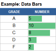
Select your range of cells, then go to Home > Conditional Formatting > Data Bars and select the style you want.

Data Bars let you create horizontal bar charts and progress bars directly within a group of cells. In the example on the right, I’m using data bars to show a histogram of class grades.

The default settings for Data Bars scale the bars automatically based on the values in the Applies To range. You can control the scale used for the bars by editing the rule’s settings. I’ll be showing a couple examples of that later in this article.

4. How to Highlight Overdue Dates

To highlight overdue dates:

Select the range of dates and go to Home > Conditional Formatting > Highlight Cells Rules > Less Than…
Enter =TODAY()+30 to highlight dates earlier than 30 days from now. Enter =TODAY() to highlight dates earlier than today.
Choose a format option from the drop-down box, then click on OK.

Examples of this technique can be found in the Equipment Calibration Log and To Do List templates.

5. How to Add Icon Sets in Excel

To add Icon Sets, select your data and then go to Home > Conditional Formatting > Icon Sets > and choose one of the options. You will amost always have to customize the settings for Icon Sets.

This example, based on the Checkbook Register Template, uses a green circle icon (⬤) to show when an account balance is >=$500, yellow/orange (⬤) when it is less than $500, and red (⬤) when the balance is negative.

After selecting the icon set from the built-in menu, you need to edit the rule to define these different values. To do that, select one of the cells in the Balance column, go to Home > Conditional Formatting > Rules Manager and click on Edit Rule. The image below shows the settings used in this example:

TIP: One of the best ways to learn how Icon Sets work is to play with all of the different drop-down options in the rule settings.

For examples of other Icon Sets, check out the Feature Comparison Template:

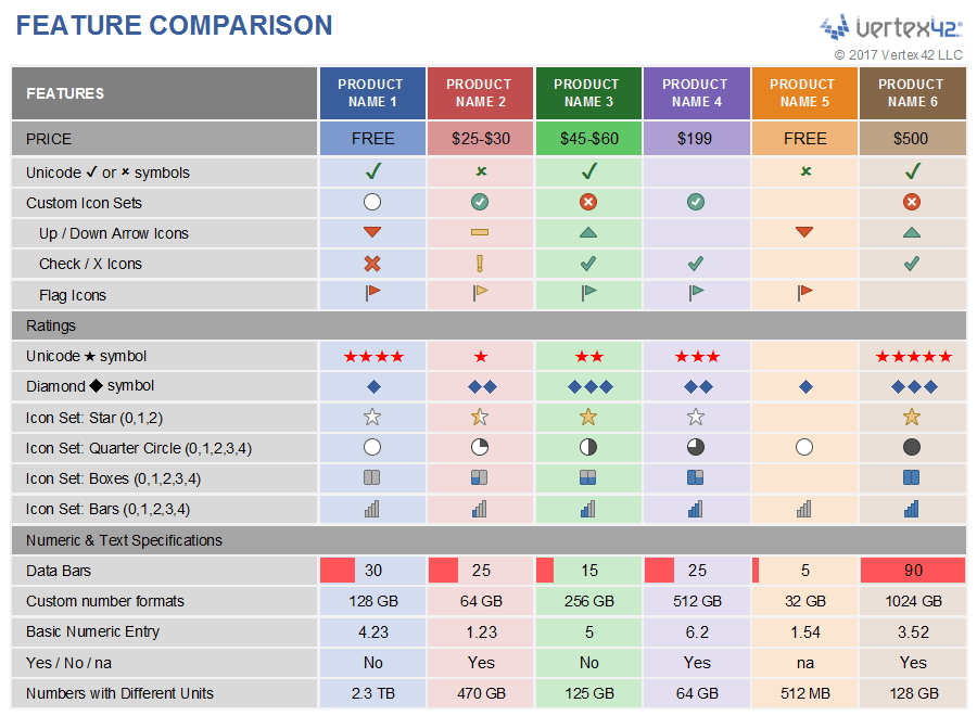
How to View/Edit Conditional Formatting Rules

Vertex42 has many templates that use both simple and advanced conditional formatting techniques. If you are using a template and want to figure out how the conditional formatting works, or want to delete or change rules, you will need to know a couple of things:

1) To view the rules for selected cells, go to Home > Conditional Formatting > Rules Manager

2) To view ALL the rules in the entire worksheet, select «This Worksheet» from the drop-down at the top of the Rules Manager window.

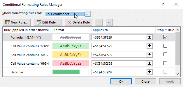
The image above shows the 5 rules used in the Task Checklist Template. The first rule changes tasks to gray strike-through when the Done column has a check mark. The next 3 rules highlight specific text in the Priority column. The last rule adds a Progress Bar in the % Complete column.

I will be using this template to demonstrate some techniques and key facts about conditional formatting, so I would recommend that you download it and experiment with it as you continue to read.

Rule Order Matters

The Task Checklist Template mentioned above demonstrates two key points about rule order or heirarchy.

Key Points

Conditional formatting rules are evaluated one at a time starting with the rule listed at the top.
A later rule cannot override the formatting already modified by a preceding rule.

Here is the list of rules again:

Key Point #2 means that if the first rule has already changed the font color to gray, the following rules cannot change the font color to green, yellow, or red. It’s first come, first serve.

In Excel, the font color and fill color (and border, and font style, and …) can be affected independently by different rules. This means that you can have one rule that changes a font to gray, a different rule that changes the cell color to red, and a different rule that adds a data bar.

Why do I need to check the Stop-If-True box?

With the Stop-If-True box checked, none of the following rules will be evaluated if the condition of that first rule is met.

That is why the first task row doesn’t show a Data Bar in the %Complete column and why the Priority «HIGH» is not highlighted red.

What would happen if I didn’t check the Stop-If-True box? Go ahead and try it … or look at the next image.

Result when Stop-if-True is Not Checked

Notice how the red fill color is applied to the HIGH cell. The first rule does not define a fill color, but it does change the font color. That means that the 4th rule can change the fill color to light red, but it can’t override the font color.

Excel vs. Google Sheets: In Excel, the Number Format, Font Color, Font Style, Font Underline, Font Effects, Fill Color, Fill Effects, Border Color, Border Style, Data Bars, and Icon Sets can be affected independently by different rules. That isn’t the case in Google Sheets. In Google Sheets, conditional formatting behaves as though all rules are Stop-If-True. Excel is much more flexible and powerful in that respect.

How to Create an In-Cell Progress Bar

You’ve already seen how to add a Data Bar, so using a Data Bar for showing progress based on a percentage is as simple as making a few changes to the Data Bar settings.

To see how it works in the Task Checklist template, go to Home > Conditional Formatting > Manage Rules, click on the Data Bar rule, then click on the Edit Rule button.

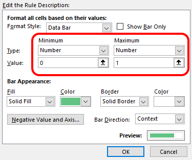
The progress should be a value between 0% and 100%. When you create a progress bar, you need to change the Minimum value to Type:Number & Value:0, and change the Maximum to Type:Number & Value:1.

NOTE Google Sheets currently doesn’t provide an in-cell data bar option. But, you can mimic the effect using the formula =REPT(«█»,ROUND(percent*10,0)).

I’ve attempted to figure out a way to change the color of the data bars conditionally, but the best I’ve been able to come up with instead is to use a 3-color scale in addition to a gray data bar. This can help if you want to use the color to signal an incomplete task.

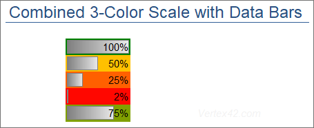
How to Highlight Every Other Row Using a Formula

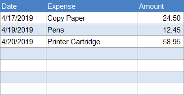
Highlighting every other row can help make tables more readable like in the expense tracking example. To do this in Excel (without needing the Tables feature), you can create a formula-based conditional formatting rule.

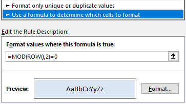
Select the cells you want to format (except the header).
Go to Home > Conditional Formatting > New Rule.
Select «Use a formula to determine which cells to format.»
Enter the formula =MOD(ROW(),2)=0.
Click on Format then select a color in the Fill tab.

Likewise, to highlight every other column, you could use the formula =MOD(COLUMN(),2)=0.

This technique allows you to insert and copy/paste rows without having to update the background colors manually, but it has one major drawback: conditional formatting overrides manual formatting.

Key Point: Conditional formatting overrides manual formatting.

This means that if you want to change the fill color of a cell in your table, but the conditional formatting rule is already changing the fill color, you won’t see the change that you are making. You ARE editing the fill color, but you won’t see the change because conditional formatting is overriding your format.

If you want to manually change the fill colors in your table AND highlight every other row, you may need to use the Format as a Table feature in Excel.

NOTE Google Sheets has a feature listed right underneath Conditional Formatting called Alternate Colors. This works separate from conditional formatting and DOES NOT override custom formatting! I LOVE that!

Conditional Formatting Based on Another Cell

To change the format of a cell based on another cell, or based on a range of cells, use a formula rule to determine which cells to format. Formulas can be simple or very complex. You can use most of the standard spreadsheet functions such as IF(), AND(), MATCH(), SEARCH(), COUNTIF(), SUMIF(), etc.

How to Create a Formula Rule

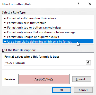
To create a formula rule, select «Use a formula to determine which cells to format» after clicking on New Rule from the Conditional Formatting menu or from within the Rule Manager.

A formula rule is activated when the formula returns TRUE.

For example, =G27<TODAY() will apply the format when the date in cell G27 is overdue (less than today’s date).

To format based on multiple conditions, use the AND() function in your formula. For example, =AND(A1>10,A1<20) will apply a format when cell A1 is between 10 and 20.

Formula Rules can be very tricky! When using relative references (references without dollar signs in front of the column letter or row number), you need to write your formula based on the top-left cell in the Applies To range. When you are creating the rule for the first time, write your formula based on the top-left cell that you have selected.

IMPORTANT: Always write the formula based on the top-left cell in the Applies To range!

How to Highlight an Entire Row

The Work Breakdown Structure template shows an example of highlighting an entire row when the value in the Level column is equal to 1.

The formula we are using is =($B6=1), and this applies to all the cells in the range $B$6:$G$30. One formula to rule them all! But how does it work?

Behind the scenes, Excel is essentially copying this formula to each of the cells in the Applies To range. When a formula is copied, relative references (no dollar sign) will change. This means that for cell C15, the formula would become =($B15=1). Column B stays the same (because of the dollar sign in front of the B), but the row changes.

Key Point: In Conditional Formatting Rules, absolute references stay the same ($B$1) and relative references (A1) change as Excel applies the formula to each cell in the Applies To range.

If you aren’t familiar with how absolute and relative references work, you may want to learn more about that. It’s absolutely critical for understanding formula-based conditional formatting.

How to Highlight Cells Based on a Range

You can use the MATCH() function within a conditional formatting formula rule to highlight cells whose values are found in another range or list.

For example, in the Yearly Event Calendar, dates are highlighted in the calendar if the date is found in the list of holidays, as shown in the image below.

The formula is =MATCH(this_date,date_range,0) where this_date is A10 (a relative reference to the top-left cell in the Applies To range), and date_range is $Y$9:$Y$300 (an absolute reference to the list of holidays in column Y).

The MATCH formula only returns TRUE if it finds this_date within date_range. (See VLOOKUP and INDEX-MATCH Examples to learn about lookup formulas).

How to Highlight Values NOT in a Range

In some spreadsheets, I use conditional formatting to highlight values that are NOT within another range. Along with Data Validation, this can help with error checking.

The formula for the rule is =ISERROR(MATCH(this_cell,other_range,0)). This returns TRUE when MATCH does not find this_cell within other_range.

I’ve used this technique in my original Money Management Template to verify budget categories.

How to Use Conditional Formatting to Create a Gantt Chart

Watch the new Video Series: How to Make a Gantt Chart in Excel!

Most of my Gantt Chart Templates use a combination of many conditional formatting rules. The example below (from the Simple Gantt Chart) demonstrates (1) how to create the bars that show the date range for each task and (2) how to show the current date using a red border.

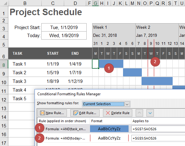
Rule 1 uses the formula =AND(task_end>=G$5,task_start<G$5+1) where task_end is a relative named range defined as $D7 and task_start is a relative named range defined as $C7. Using named ranges isn’t necessary. The formula could be written as =AND($D7>=G$5,$C7<G$5+1)

Rule 2 can use the same formula, with today’s date in place of both task_end and task_start. Or, the rule could be as simple as =G$5=TODAY().

The proper use of absolute and relative ranges is absolutely critical here. So, pay special attention to the placement of the dollar signs.

Note You may notice that row 7 is hidden in the screenshot. The reason for hiding the first row of the gantt chart is so that if a person inserts a row above row 8, it will use the formatting from row 7 rather than the formatting from row 6.

Using a «No-Format Stop» Rule

In some of my Gantt charts, such as the Construction Schedule, the user can pick the color of each bar. Each different color requires a separate conditional formatting rule.

One way to do this would be to add the color condition to each rule like this: =AND($D7=»red»,task_end>=G$5,task_start<G$5+1).

However, I often prefer to use what I call a «No-Format Stop» Rule. Instead of saying where you want the color to be applied, this rule defines where the color should NOT be, and stops if true.

This No-Format Stop rule can be as simple as adding NOT() around the main gantt chart rule like this =NOT(AND(task_end>=G$5,task_start<G$5+1)). It’s called a «No-Format» rule because no formatting is applied. Its only purpose is to prevent the rules that come after it from being applied.

The following rules then need to only check for what color to assign. In the example, the color is entered in column D. When cell D7 is blank, the bar will be gray. When D7=»B», the bar will be blue … and so on.

Use Data Bars to Compare Two Groups

Charts like the population example below are popular for comparing two different groups.

The trick to creating a chart like this with Data Bars is to use two different columns. The settings for the Male column use the «Right-to-Left» direction as shown in the image below.

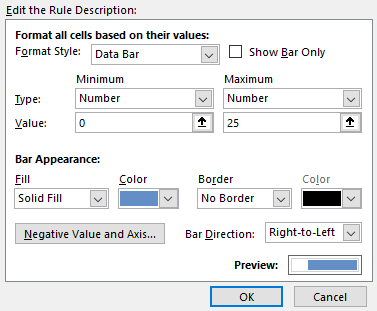
!!! The column widths and the Min/Max values need to be identical for both columns of data, or the visual display will misrepresent the numbers. In this case, the Minimum is 0 and the Maximum is 25 for both the blue data bars and the red data bars.

You could argue that this type of graph is not ideal for making exact comparisons between the Male and Female population. For example, if the numbers weren’t included in the chart, could you tell that for Age 40 to 49 there were more females (20.48 vs. 20.14)? No, you couldn’t. The bars look like they are the same length.

Our brains make better length comparisons when two things are aligned and parallel. The next chart uses Data Bars arranged a little differently. Now you CAN see the difference between the Male and Female population.

Control Scaling by Linking Min/Max to Cells

A great solution for controlling the scaling for Data Bars and Color Scales is to link the Minimum and Maximum values to cells that you can edit. Using this approach, you can have different rules using the same Min/Max values. Here’s an example:

To do this, edit the rule settings with cell references like this:

The green data bar and blue data bars in this example are separate rules, but both rules use Min/Max values linked to cells C139 and D139.

Change Number Formats via Conditional Formatting

Some tricks I like to use in my templates involve changing the custom number format via conditional formatting based on user-selected options. If you aren’t already familiar with how to create custom number formats, I would encourage you to read the article Custom Number Formats in Excel.

Suffice it to say for now that you assign custom number formats by going to the Number tab when editing the Format for a conditional formatting rule.

Change Date Formats to d/m/yyyy

If you are sharing a file with people from different countries, you may want a simple way to switch the display of dates from m/d/y to d/m/y. I use this technique in Gantt Chart Template Pro.

The date in cell F131 displays a date as m/d/yyyy by default, but when the user selects «dmy» in cell D131, the CF rule changes the format to d/m/yyyy.

You could set up similar options to switch time formats between standard and 24-hour time, or change the display of numbers from decimal to fractions.

Note Developers: To avoid having to switch between date formats, use the built-in date formats marked with the asterisk (*) when you can. From Excel: «Date formats that begin with an asterisk (*) respond to changes in regional date and time settings that are specified for the operating system.»

Hide Zero Values

This example shows 3 different ways to hide zero values using conditional formatting.

The 2nd column hides the zero values by changing the font color to white.
The 3rd column changes the custom number format to » — «.
The 3rd column changes the custom number format to » «.

I personally prefer replacing zeros with a dash because otherwise the cell looks blank, and cells that look blank tend to be deleted or overwritten because you think they are empty.

Automatic Indenting

A custom number format will allow you to add text characters before or after the number, so you can simulate indenting by adding a number of spaces before your text using the format code » «@.

I use this technique in both the free Work Breakdown Structure template, and the premium Gantt Chart Template.

In this example, the formula is counting the number of decimal points in the WBS number. One rule adds 3 spaces before the text if it finds 1 decimal point. A second rule adds 6 spaces before the text if it finds 2 decimal points. See the article Text Manipulation Formulas to learn how this formula counts decimal places.

Display 23K, 23M, or 23B Based on the Value

Displaying large numbers as thousands, millions, or billions is VERY common, but how do you automatically display «K» or «M» or «B» depending on the value of the number? Using 3 different CF rules with the custom format codes 0.0K, 0.0M, and 0.0B.

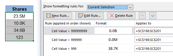
Display Custom Icons

Excel has a limited number of icons available for Icon Sets. However, if you use unicode symbols and emojis, you can create your own icons using multiple CF rules. The format codes in this example are simply 0* X where X is the unicode character. To place the icon on the left with the number on the right, you could use X* 0.00 instead.

Check out the Moon Phase Calendar to see how it uses conditional formatting to replace dates in a calendar with moon phase unicode characters.

How to Copy Conditional Formatting

The simple answer is that unless you tell Excel or Google Sheets NOT to, conditional formatting will be copied whenever other formatting is copied. For example, when you copy/paste cells, when you use the format painter tool, and when you insert rows and columns.

Copying conditional formatting may not always behave the way you expect it to. Sometimes that may not matter, but in other cases it may cause significant errors in how the data is interpreted. So, it’s always a good idea to check your conditional formatting rules after copying/pasting.

One of the main problems I’ve seen occurs when copying a row and inserting the copied row. Rules may be split, resulting in separate rules for different ranges when you expect there to be only one rule for the entire range. This can cause problems with color scales and data bars, especially.

To avoid the problem of splitting CF rules, when pasting you can use Paste Special and choose the «All Merging Conditional Formats» option.

Conditional Formatting is Volatile

If you use a lot of conditional formatting in your worksheet, or the rules involve inefficient formulas, you may notice Excel appear to slow down. That is because Conditional Formatting is volatile — meaning that the rules are evaluated every time the display refreshes.

To experiment with this concept, I built the following example. The fire in the display will flicker every time rules are evaluated, allowing you to test actions that cause the display to refresh.

Download the Example File (VolatileCF.xlsx)

Wrap Up and Final Tips

If you like this article, or use some of these ideas, please share the link to this article via your website and social media!

I didn’t talk about all the possible uses for conditional formatting, and not even some of the most common uses, such as making negative values red and highlighting based on specific text values. That is partly because many of these techniques are extremely easy to implement using the built-in options.

If you have questions, please go ahead and submit a comment below.

If you’d like to try some geeky fun, check out the Mine Blaster 1000 game. It makes use of multiple overlapping conditional formatting rules to create a game something roughly like Minesweeper (without any VBA).

Источник

How to Use Conditional Formatting to Highlight Text in Excel

Conditional formatting in Excel is formatting that changes with the cell content.

That means you don’t have to change it when the cell content changes.

You use conditional formatting to make it easier for the user to identify key points of interest.

That could be:

All cells that contain the name of a certain employee
All rows regarding a certain order number

Or a lot of other things.

Follow this step-by-step guide and learn to highlight text with conditional formatting in Excel.

And a bit more😉

Download the workbook I use in this guide if you want to tag along.

Highlight text with conditional formatting

The reason for highlighting text with conditional formatting is to draw the user’s attention to those cells – so they find relevant information faster🏃

You apply conditional formatting with what is called conditional formatting rules.

It’s really easy to insert one of those.

1. Select all the cells where the text you want to highlight can be.

In the sample data, I want to identify all L compatible adapters. So, I select all cells in column B (from cell B2 and down).

Conditional formatting in Excel - Selected cells for highlight cells rules

2. In the middle of the Home tab, click ‘Conditional Formatting’.

Click conditional formatting button in Excel

3. Hover your cursor over ‘Highlight Cells Rules’ and select ‘Text that Contains’.

Conditional formatting in Excel - click highlight cells rules

4. In the dialog box that appears, write the text you want to highlight, in the left field.

Conditional formatting in Excel - Write text for criteria

As you type it, you can see the conditional formatting applied instantly.

The formatting being applied is the standard conditional formatting format.

5. To change the format, click the drop-down arrow in the right field and select another of the formatting presets.

6. Or you can create your own format by clicking ‘Custom format’.

Conditional formatting in Excel - Custom formatting style

7. After clicking ‘Custom Format’ the ‘Format Cells’ dialog box appears.

This is the same as the normal ‘Format Cells’ dialog box you’re using when you apply normal formatting in a spreadsheet.

Use whatever formatting style you want for your conditional formatting rule.

Conditional formatting in Excel - Format cells to get your formatting style

And that’s it!

Now, all cells containing the text “L compatible” are highlighted with the chosen formatting.

Conditional formatting in Excel - highlight cells

Because conditional formatting is dynamic, it changes when the data changes. So if the content of a cell changes from whatever to “L compatible” that cell gets highlighted too.

Kasper Langmann, Microsoft Office Specialist

Highlight numbers with conditional formatting

Sometimes you’re not reading all your data in your sheets, you’re just looking for specific numbers.

That can be a tedious process, especially if you have a large data set.

Let’s dive into our inventory list again🤿

If the quantity in stock of an item reaches below 100 it’s critical that you find out, so you can buy more units of that particular item.

Let’s make a simple conditional formatting rule to highlight cells.

1. Select the cells in the quantity column (cells C2 and down).

Conditional formatting in Excel - select quantity cells

With those selected cells, we need to apply a ‘Highlight Cells’ conditional formatting rule.

2. In the Home tab of the ribbon, click ‘Conditional Formatting’.

3. Hold your cursor over ‘Highlight Cells Rules’ and click ‘Less than’.

Click Conditional formatting in Excel - highlight cells rules

This conditional formatting rule allows you to apply conditional formatting if the value of a cell is less than what you’re defining in a few seconds.

4. In the left field, write the number the cell value should be less than to apply conditional formatting.

Click Conditional formatting in Excel - click highlight cells rules less than value

As you type, you can see the format of this conditional formatting rule being applied to the selected cells.

Right now, it’s just the standard format: Light Red Fill with Dark Red Text.

Classic👍

5. In the right field, click the drop-down button if you want to change to another formatting preset.

Choose formatting for the highlighted cells

6. Or you can click ‘Custom Format’ to control the formatting style 100%.

Conditional formatting - format cells box

And that’s it.

Watch all the values below 100 being highlighted automatically. Beautiful, isn’t it?💕

Conditional formatting in Excel - highlight values

This conditional formatting rule can be modified to other situations if you take a step back.

For instance, you can turn it upside down and highlight cells that are above 100.

Or cells with values between 50 and 150.

The possibilities are almost endless.

Highlighting entire rows based on a formula

Entire rows look nice when they are formatted in a certain way. Instead of random colored cells everywhere.

So, let me show you how to color an entire row with a conditional formatting rule if the value in column C is less than 100👀

1. Select the entire data set. The selected cells indicate how much of each row is highlighted by the conditional formatting rule.

2. Click ‘Conditional Formatting’ on the Home tab and click ‘New Rule.’

Click conditional formatting in Excel - new rule

3. In the dialog box that appears, select ‘Use a formula to determine which cells to format’ from the ‘Rule Type’ menu.

Conditional formatting in Excel - new rule from formula

4. Right below, enter this formula:

=$C1<100

So, if the value in column C drops below 100, the conditional formatting rule triggers.

You can’t refer to entire columns, so you need to refer to C1. NOT C2, although it seems more logical⚙️

If your data starts in row 3, 5, 10, or whatever other row, the reference still goes to C1 (or whatever column you’re using).

5. Now chose your formatting style from the ‘Custom Format’ button.

Or settle for the standard preset.

And behold!

All the cells in your data rows are now formatted, and not just in 1 column like they typically are with conditional formatting.

Conditional formatting in Excel - highlight entire row based on value

Editing and removing conditional formatting rules

The layout and use of a workbook are rarely static, so the conditional formatting that you apply to your sheet may have to be edited at some point.

For instance, the previous highlight cells rules we set… Maybe it’s time to change them.

Luckily that’s fairly easy.

You can edit any conditional formatting rule from the conditional formatting rules manager.

Edit the conditional formatting rule and formatting style

1. Click ‘Conditional Formatting’ from the Home tab and select ‘Manage Rules’.

Click conditional formatting and Manage Rules

After you click ‘Manage Rules…’ you’ll see a ‘Conditional Formatting Rules Manager’ dialog box.

Change the following 3 points as you see them on in the manager.

2. Set ‘Show formatting rules for:’ to ‘This Worksheet’ to show all conditional formatting rules for the entire sheet.

3. Find the rule you want to edit (there might be several on the list).

4. Click the ‘Edit Rule’ button.

Another dialog box appears. From here you can change anything about the rule.

Conditional formatting - Edit formatting rule dialog box

Below we’ll go through the different options shown in the screenshot above.

Circle 1) Here you can change the ‘Rule Type’. If you don’t want to apply conditional formatting when “something” happens in a cell, you can change it to apply on all cells and fill them with color based on their value compared to the average of the data.

Circle 2) If you keep the ‘Rule Type’ you can change the “trigger” of the formatting. The trigger depends entirely on which type of conditional formatting rule you choose in circle 1. In this case, you can change the custom formula.

Circle 3) From this little (familiar) box you can change the formatting that you applied in the first place. If you don’t want your cells to turn yellow when it drops below cell value: 100, you can have them turn purple instead.

As you see there are more than enough options.

But wait – there’s more!

Edit the conditional formatting rules range

All of the above is very nice, but if you accidentally selected the wrong area when you made the conditional formatting rule – then it doesn’t help to change the ‘Rule Type’ or whether the cells should be red or blue.

And if you spent 5 minutes entering a unique formula to “trigger” the formatting, then it sucks to delete it and do it all over.

To change the range of cells that the conditional formatting applies to, you don’t need to go to the ‘Edit Rule’ box above.

You just need to click in the ‘Applies to’ column at the rule you want to change in the ‘Conditional Formatting Rules Manager’ box.

Conditional formatting edit selected range

If you can’t remember the range that the rule should apply to, click the tiny red arrow to select the range manually.

That’s how you edit a conditional formatting rule✏️

So if you screw one up?

You don’t have to delete it – simply just edit it.

Delete a conditional formatting rule

Sometimes you see a workbook with too many conditional formatting rules.

This can create immense confusion and on top of that, it can make your workbook slow.

In this case, you need to remove conditional formatting from the spreadsheet. Maybe even all of it!

Click the ‘Conditional Formatting’ button on the ‘Home’ tab and hover your mouse over ‘Clear Rules’.

Click conditional formatting clear rules

Then click ‘Clear Rules from Entire Sheet’.

That was pretty easy. But it’s not always clever to clear all conditional formatting rules from a sheet!

Sometimes some rules should still apply.

To select specifically which conditional formatting rules are to be removed, click ‘Manage Rules…’ instead.

Click manage rules to start to clear rules

Here you’ll find the conditional formatting rules manager dialog box that you can use to clear rules, in addition to editing rules.

To delete specific conditional formatting rules:

Click on 'Delete Rule' from 'Rules Manager' dialog box to clear conditional format

Click the drop-down arrow that initially says “Current Selection”. Change it to “This Worksheet”.
Select the conditional formatting rule you don’t want anymore.
Press ‘Delete Rule’ to actually clear rules.

Remember to click OK when you’re done.

And that’s how you actually clear rules✏️

That’s it – Now what?

That’s how to highlight cells with conditional formatting.

Like all the cells that contain a specific word or a number.

Heck, you even learned how to remove conditional formatting, create a new rule from a formula, and much more.

Well done💪

Conditional formatting is a part of Excel that can think for itself. Meaning it makes its own decisions. It “reads” the cell and reacts on the content.

There are several other parts of Excel that react to the content of cells – just like conditional formatting does.

And you most definitely want to learn those parts.

So, I’ve made a free course teaching you 2 of the best conditional functions Excel has to offer: IF and SUMIF.

Also, you learn VLOOKUP and pivot tables.

Click here to enroll in my free 30-minute course and I’ll send it to your inbox right away.

Frequently Asked Questions

If you’re looking for a specific answer to a specific question, please see the FAQ section below. Maybe you’ll find what you need😊

Conditional Formatting is formatting that changes when the cell that it’s based on changes.

This is very different from normal formatting which is static and does not change unless you make the change yourself.

For example, you can make a cell change color when its content drops below 100.

Conditional formatting is located on the Home tab on the Ribbon in Excel. The Ribbon is the main menu, on the top of your screen, where most Excel features are accessible from buttons.

Select your data and click the conditional formatting button to use any of the conditional formatting rules.

Yes, you can use the format painter to copy and paste conditional formatting quite easily.

Select the cells with conditional formatting and from the Home tab, click the ‘Format painter‘ button.

Then select the cells where you want to paste conditional formatting.

Kasper Langmann2023-02-23T11:25:29+00:00

Page load link

Источник

Conditional formatting in Excel is used more often because of its useful characteristics. When you need to apply formats to the dataset, conditional formatting is used. Not only this, but you can even highlight the data in the sheet to identify the changes in cell values.

For beginners, conditional formatting sometimes could be complex and vague. For some users, this feature is not a favorite one that’s why often users tend to avoid it. However, this feature is not difficult at all. And it does not take much time. But do you know how to do conditional formatting in Excel? Let’s understand this in detail.

Conditional Formatting Overview

With conditional formatting, you can apply formatting by default such as icons, colors, and data bars. You can apply formatting to one or more cells and it all depends on the cell value. For this, you need to make a conditional formatting rule. Suppose, you have a value less than $2000, and the cell color is red. Once you apply this rule, you can easily find which cells have values less than $2000.

What is Conditional Formatting in Excel?

When you need to apply particular formatting to data that matches one or more conditions, conditional formatting is then used. Similar to standard formatting, you can highlight as well as distinguish data in several ways since it changes the fill color, font color, and border styles of a cell. Generally, this feature is much more dynamic and supple. Conditional formatting is updated by default once the data is changed to reflect the changes.

You can apply conditional formatting to individual cells or entire rows on the bases of the value given in the formatted cell. Preset rules are used to apply conditional format on your data and these rules include data bars, icon sets, color scales, or even you can personalize rules.

How to Do Conditional Formatting in Excel (Highlighting Text)

When you intend to highlight text by using conditional formatting, it simply shows that you need to divert the attention of the users to the cells containing relevant data. You can follow the steps given below to add one of the rules used in conditional formatting:

Select all the cells in which the text is needed to highlight.
Here in this example, we will select all cells in column B.

Open the Home tab and choose the Conditional Formatting option.

Place the cursor over the “Highlight Cells Rules” option and choose the “Text that Contains” option.

A dialog box will appear in which you need to add the text that needed to be highlighted in the left field.

You will instantly notice the conditional formatting is applied as you enter the text.
The formatting you notice will be standard but you can make changes to it the way you need.
For this, click on the drop-down arrow given in the right field and choose another formatting preset.
Or else, you can make a new format by clicking on the custom format.

Once you click on the Custom Format, you will see a Format Cells dialog box. This dialog box is a normal one as you have applied formatting in a sheet. You can choose whatever formatting style you need.

All set!

Now, you will see all the selected cells are under the effect of the conditional formatting you have applied.

That’s it!

That’s all, now what comes next?

You understand how to do conditional formatting in Excel. Basically, conditional formatting is an important part of the Excel tool that does not need instructions once you create it properly. It by default reviews the cell and responds accordingly.

Источник