
Excel for Microsoft 365 Excel for Microsoft 365 for Mac Excel for the web Excel 2021 Excel 2021 for Mac Excel 2019 Excel 2019 for Mac Excel 2016 Excel 2016 for Mac Excel 2013 Excel Web App Excel 2010 Excel 2007 Excel for Mac 2011 Excel Starter 2010 More…Less
You can use the IFERROR function to trap and handle errors in a formula. IFERROR returns a value you specify if a formula evaluates to an error; otherwise, it returns the result of the formula.
Syntax
IFERROR(value, value_if_error)
The IFERROR function syntax has the following arguments:
-
value Required. The argument that is checked for an error.
-
value_if_error Required. The value to return if the formula evaluates to an error. The following error types are evaluated: #N/A, #VALUE!, #REF!, #DIV/0!, #NUM!, #NAME?, or #NULL!.
Remarks
-
If value or value_if_error is an empty cell, IFERROR treats it as an empty string value («»).
-
If value is an array formula, IFERROR returns an array of results for each cell in the range specified in value. See the second example below.
Examples
Copy the example data in the following table, and paste it in cell A1 of a new Excel worksheet. For formulas to show results, select them, press F2, and then press Enter.
|
Quota |
Units Sold |
|
|---|---|---|
|
210 |
35 |
|
|
55 |
0 |
|
|
23 |
||
|
Formula |
Description |
Result |
|
=IFERROR(A2/B2, «Error in calculation») |
Checks for an error in the formula in the first argument (divide 210 by 35), finds no error, and then returns the results of the formula |
6 |
|
=IFERROR(A3/B3, «Error in calculation») |
Checks for an error in the formula in the first argument (divide 55 by 0), finds a division by 0 error, and then returns value_if_error |
Error in calculation |
|
=IFERROR(A4/B4, «Error in calculation») |
Checks for an error in the formula in the first argument (divide «» by 23), finds no error, and then returns the results of the formula. |
0 |
Example 2
|
Quota |
Units Sold |
Ratio |
|---|---|---|
|
210 |
35 |
6 |
|
55 |
0 |
Error in calculation |
|
23 |
0 |
|
|
Formula |
Description |
Result |
|
=C2 |
Checks for an error in the formula in the first argument in the first element of the array (A2/B2 or divide 210 by 35), finds no error, and then returns the result of the formula |
6 |
|
=C3 |
Checks for an error in the formula in the first argument in the second element of the array (A3/B3 or divide 55 by 0), finds a division by 0 error, and then returns value_if_error |
Error in calculation |
|
=C4 |
Checks for an error in the formula in the first argument in the third element of the array (A4/B4 or divide «» by 23), finds no error, and then returns the result of the formula |
0 |
|
Note: If you have a current version of Microsoft 365, then you can input the formula in the top-left-cell of the output range, then press ENTER to confirm the formula as a dynamic array formula. Otherwise, the formula must be entered as a legacy array formula by first selecting the output range, input the formula in the top-left-cell of the output range, then press CTRL+SHIFT+ENTER to confirm it. Excel inserts curly brackets at the beginning and end of the formula for you. For more information on array formulas, see Guidelines and examples of array formulas. |
Need more help?
You can always ask an expert in the Excel Tech Community or get support in the Answers community.
Need more help?
Return value
The value you specify for error conditions.
Usage notes
The IFERROR function is used to catch errors and return a more friendly result or message when an error is detected. When a formula returns a normal result, the IFERROR function returns that result. When a formula returns an error, IFERROR returns an alternative result. IFERROR is an elegant way to trap and manage errors. The IFERROR function is a modern alternative to the ISERROR function.
Use the IFERROR function to trap and handle errors produced by other formulas or functions. IFERROR checks for the following errors: #N/A, #VALUE!, #REF!, #DIV/0!, #NUM!, #NAME?, or #NULL!.
Example #1
In the example shown, the formula in E5 copied down is:
=IFERROR(C5/D5,0)
This formula catches the #DIV/0! error that occurs when Qty is empty or zero, and replaces it with zero.
Example #2
For example, if A1 contains 10, B1 is blank, and C1 contains the formula =A1/B1, the following formula will catch the #DIV/0! error that results from dividing A1 by B1:
=IFERROR (A1/B1,"Please enter a value in B1")
As long as B1 is empty, C1 will display the message «Please enter a value in B1» if B1 is blank or zero. When a number is entered in B1, the formula will return the result of A1/B1.
Example #3
You can also use the IFERROR function to catch the #N/A error thrown by VLOOKUP when a lookup value isn’t found. The syntax looks like this:
=IFERROR(VLOOKUP(value,data,column,0),"Not found")
In this example, when VLOOKUP returns a result, IFERROR functions that result. If VLOOKUP returns #N/A error because a lookup value isn’t found, IFERROR returns «Not Found».
IFERROR or IFNA?
The IFERROR function is a useful function, but it is a blunt instrument since it will trap many kinds of errors. For example, if there’s a typo in a formula, Excel may return the #NAME? error, but IFERROR will suppress the error and return the alternative result. This can obscure an important problem. In many cases, it makes more sense to use the IFNA function, which only traps the #N/A error.
Other error functions
Excel provides a number of error-related functions, each with a different behavior:
- The ISERR function returns TRUE for any error type except the #N/A error.
- The ISERROR function returns TRUE for any error.
- The ISNA function returns TRUE for #N/A errors only.
- The ERROR.TYPE function returns the numeric code for a given error.
- The IFERROR function traps errors and provides an alternative result.
- The IFNA function traps #N/A errors and provides an alternative result.
Notes
- If value is empty, it is evaluated as an empty string («») and not an error.
- If value_if_error is supplied as an empty string («»), no message is displayed when an error is detected.
- In Excel 2013+, you can use the IFNA function to trap and handle #N/A errors specifically.
Содержание
- How to correct a #VALUE! error in the IF function
- Problem: The argument refers to error values
- Problem: The syntax is incorrect
- Need more help?
- IFERROR function
- Syntax
- Remarks
- Examples
- Example 2
- Need more help?
- Функция IFERROR (ЕСЛИОШИБКА) в Excel. Как использовать?
- Видеоурок
- Что возвращает функция
- Синтаксис
- Аргументы функции
- Дополнительная информация
- Примеры использования функции IFERROR (ЕСЛИОШИБКА) в Excel
- Пример 1. Заменяем ошибки в ячейке на пустые значения
- Пример 2. Заменяем значения без данных при использовании функции VLOOKUP (ВПР) на “Не найдено”
- Пример 3. Возвращаем значение “0” вместо ошибок формулы
- IF function
- Simple IF examples
- Common problems
- Need more help?
- IFERROR Function
- Related functions
- Summary
- Purpose
- Return value
- Arguments
- Syntax
- Usage notes
- Example #1
- Example #2
- Example #3
- IFERROR or IFNA?
- Other error functions
How to correct a #VALUE! error in the IF function
IF is one of the most versatile and popular functions in Excel, and is often used multiple times in a single formula, as well as in combination with other functions. Unfortunately, because of the complexity with which IF statements can be built, it is fairly easy to run into the #VALUE! error. You can usually suppress the error by adding error-handling specific functions like ISERROR, ISERR, or IFERROR to your formula.
Problem: The argument refers to error values
When there is a cell reference to an error value, IF displays the #VALUE! error.
Solution: You can use any of the error-handling formulas such as ISERROR, ISERR, or IFERROR along with IF. The following topics explain how to use IF, ISERROR and ISERR, or IFERROR in a formula when your argument refers to error values.
IFERROR was introduced in Excel 2007, and is far more preferable to ISERROR or ISERR, as it doesn’t require a formula to be constructed redundantly. ISERROR and ISERR force a formula to be calculated twice, first to see if it evaluates to an error, then again to return its result. IFERROR only calculates once.
=IFERROR(Formula,0) is much better than =IF(ISERROR(Formula,0,Formula))
Problem: The syntax is incorrect
If a function’s syntax is not constructed correctly, it can return the #VALUE! error.
Solution: Make sure you are constructing the syntax properly. Here’s an example of a well-constructed formula that nests an IF function inside another IF function to calculate deductions based on income level.
=IF(E2 IF(the value in cell A5 is less than 31,500, then multiply the value by 15%. But IF it’s not, check to see if the value is less than 72,500. IF it is, multiply by 25%, otherwise multiply by 28%).
To use IFERROR with an existing formula, you just wrap the completed formula with IFERROR:
=IFERROR(IF(E2 Note: The evaluation values in formulas don’t have commas. If you add them, the IF function will try to use them as arguments and Excel will yell at you. On the other hand, the percentage multipliers have the % symbol. This tells Excel you want those values to be seen as percentages. Otherwise, you would need to enter them as their actual percentage values, like “E2*0.25”.

Need more help?
You can always ask an expert in the Excel Tech Community or get support in the Answers community.
Источник
IFERROR function
You can use the IFERROR function to trap and handle errors in a formula. IFERROR returns a value you specify if a formula evaluates to an error; otherwise, it returns the result of the formula.
Syntax
The IFERROR function syntax has the following arguments:
value Required. The argument that is checked for an error.
value_if_error Required. The value to return if the formula evaluates to an error. The following error types are evaluated: #N/A, #VALUE!, #REF!, #DIV/0!, #NUM!, #NAME?, or #NULL!.
If value or value_if_error is an empty cell, IFERROR treats it as an empty string value («»).
If value is an array formula, IFERROR returns an array of results for each cell in the range specified in value. See the second example below.
Examples
Copy the example data in the following table, and paste it in cell A1 of a new Excel worksheet. For formulas to show results, select them, press F2, and then press Enter.
=IFERROR(A2/B2, «Error in calculation»)
Checks for an error in the formula in the first argument (divide 210 by 35), finds no error, and then returns the results of the formula
=IFERROR(A3/B3, «Error in calculation»)
Checks for an error in the formula in the first argument (divide 55 by 0), finds a division by 0 error, and then returns value_if_error
Error in calculation
=IFERROR(A4/B4, «Error in calculation»)
Checks for an error in the formula in the first argument (divide «» by 23), finds no error, and then returns the results of the formula.
Example 2
Error in calculation
Checks for an error in the formula in the first argument in the first element of the array (A2/B2 or divide 210 by 35), finds no error, and then returns the result of the formula
Checks for an error in the formula in the first argument in the second element of the array (A3/B3 or divide 55 by 0), finds a division by 0 error, and then returns value_if_error
Error in calculation
Checks for an error in the formula in the first argument in the third element of the array (A4/B4 or divide «» by 23), finds no error, and then returns the result of the formula
Note: If you have a current version of Microsoft 365, then you can input the formula in the top-left-cell of the output range, then press ENTER to confirm the formula as a dynamic array formula. Otherwise, the formula must be entered as a legacy array formula by first selecting the output range, input the formula in the top-left-cell of the output range, then press CTRL+SHIFT+ENTER to confirm it. Excel inserts curly brackets at the beginning and end of the formula for you. For more information on array formulas, see Guidelines and examples of array formulas.
Need more help?
You can always ask an expert in the Excel Tech Community or get support in the Answers community.
Источник
Функция IFERROR (ЕСЛИОШИБКА) в Excel. Как использовать?
Функция IFERROR (ЕСЛИОШИБКА) в Excel лучше всего подходит для обработки случаев, когда формулы возвращают ошибку. Используя эту функцию, вы можете указать, какое значение функция должна возвращать вместо ошибки. Если функция в ячейке не возвращает ошибку, то возвращается её собственный результат.
Видеоурок
Что возвращает функция
Указанное вами значение, в случае если в ячейке есть ошибка.
Синтаксис
=IFERROR(value, value_if_error) — английская версия
=ЕСЛИОШИБКА(значение;значение_если_ошибка) — русская версия
Аргументы функции
- value (значение) — это аргумент, который проверяет, есть ли в ячейке ошибка. Обычно, ошибкой может быть результат какого либо вычисления;
- value_if_error (значение_если_ошибка) — это аргумент, который заменяет ошибку в ячейке (в случае её наличия) на указанное вами значение. Ошибки могут выглядеть так: #N/A, #REF!, #DIV/0!, #VALUE!, #NUM!, #NAME?, #NULL! (английская версия Excel) или #ЗНАЧ!, #ДЕЛ/0, #ИМЯ?, #Н/Д, #ССЫЛКА!, #ЧИСЛО!, #ПУСТО! (русская версия Excel).
Дополнительная информация
- Если вы используете кавычки («») в качестве аргумента value_if_error (значение_если_ошибка), ячейка ничего не отображает в случае ошибки.
- Если аргумент value (значение) или value_if_error (значение_если_ошибка) ссылается на пустую ячейку, она рассматривается как пустая.
Примеры использования функции IFERROR (ЕСЛИОШИБКА) в Excel
Пример 1. Заменяем ошибки в ячейке на пустые значения
Если вы используете функции, которые могут возвращать ошибку, вы можете заключить ее в функцию и указать пустое значение, возвращаемое в случае ошибки.
В примере, показанном ниже, результатом ячейки D4 является # DIV/0!.
![]()
Для того, чтобы убрать информацию об ошибке в ячейке используйте эту формулу:
=IFERROR(A1/A2,””) — английская версия
=ЕСЛИОШИБКА(A1/A2;»») — русская версия
![]()
В данном случае функция проверит, выдает ли формула в ячейке ошибку, и, при её наличии, выдаст пустой результат.
В качестве результата формулы, исправляющей ошибки, вы можете указать любой текст или значение, например, с помощью следующей формулы:
=IFERROR(A1/A2,”Error”) — английская версия
=ЕСЛИОШИБКА(A1/A2;»») — русская версия
![]()
Если вы пользуетесь версией Excel 2003 или ниже, вы не найдете функцию IFERROR (ЕСЛИОШИБКА) . Вместо нее вы можете использовать обычную функцию IF или ISERROR.
Пример 2. Заменяем значения без данных при использовании функции VLOOKUP (ВПР) на “Не найдено”
Когда мы используем функцию VLOOKUP (ВПР) , часто сталкиваемся с тем, что при отсутствии данных по каким либо значениям, формула выдает ошибку “#N/A”.
На примере ниже, мы хотим с помощью функции VLOOKUP (ВПР) для выбранных студентов подставить данные из результатов экзамена.
![]()
На примере выше, в списке студентов с результатами экзамена нет данных по имени Иван, в результате, при использовании функции VLOOKUP (ВПР) , формула нам выдает ошибку.
Как раз в этом случае мы можем воспользоваться функцией IFERROR (ЕСЛИОШИБКА) , для того, чтобы результат вычислений выглядел корректно, без ошибок. Добиться этого мы можем с помощью формулы:
=IFERROR(VLOOKUP(D2,$A$2:$B$12,2,0),”Не найдено”) — английская версия
=ЕСЛИОШИБКА(ВПР(D2;$A$2:$B$12;2;0);»Не найдено») — русская версия
![]()
Пример 3. Возвращаем значение “0” вместо ошибок формулы
Если у вас нет конкретного значения, которое вы бы хотели использовать для замены ошибок — оставляйте аргумент функции value_if_error (значение_если_ошибка) пустым, как показано на примере ниже и в случае наличия ошибки, функция будет выдавать “0”:
Источник
IF function
The IF function is one of the most popular functions in Excel, and it allows you to make logical comparisons between a value and what you expect.
So an IF statement can have two results. The first result is if your comparison is True, the second if your comparison is False.
For example, =IF(C2=”Yes”,1,2) says IF(C2 = Yes, then return a 1, otherwise return a 2).

Use the IF function, one of the logical functions, to return one value if a condition is true and another value if it’s false.
IF(logical_test, value_if_true, [value_if_false])
The condition you want to test.
The value that you want returned if the result of logical_test is TRUE.
The value that you want returned if the result of logical_test is FALSE.
Simple IF examples

In the above example, cell D2 says: IF(C2 = Yes, then return a 1, otherwise return a 2)

In this example, the formula in cell D2 says: IF(C2 = 1, then return Yes, otherwise return No)As you see, the IF function can be used to evaluate both text and values. It can also be used to evaluate errors. You are not limited to only checking if one thing is equal to another and returning a single result, you can also use mathematical operators and perform additional calculations depending on your criteria. You can also nest multiple IF functions together in order to perform multiple comparisons.
 B2,”Over Budget”,”Within Budget”)» loading=»lazy»>
=IF(C2>B2,”Over Budget”,”Within Budget”)
In the above example, the IF function in D2 is saying IF(C2 Is Greater Than B2, then return “Over Budget”, otherwise return “Within Budget”)
 B2,C2-B2,»»)» loading=»lazy»>
In the above illustration, instead of returning a text result, we are going to return a mathematical calculation. So the formula in E2 is saying IF(Actual is Greater than Budgeted, then Subtract the Budgeted amount from the Actual amount, otherwise return nothing).

In this example, the formula in F7 is saying IF(E7 = “Yes”, then calculate the Total Amount in F5 * 8.25%, otherwise no Sales Tax is due so return 0)
Note: If you are going to use text in formulas, you need to wrap the text in quotes (e.g. “Text”). The only exception to that is using TRUE or FALSE, which Excel automatically understands.
Common problems
What went wrong
There was no argument for either value_if_true or value_if_False arguments. To see the right value returned, add argument text to the two arguments, or add TRUE or FALSE to the argument.
This usually means that the formula is misspelled.
Need more help?
You can always ask an expert in the Excel Tech Community or get support in the Answers community.
Источник
IFERROR Function

Summary
The Excel IFERROR function returns a custom result when a formula generates an error, and a standard result when no error is detected. IFERROR is an elegant way to trap and manage errors without using more complicated nested IF statements.
Purpose
Return value
Arguments
- value — The value, reference, or formula to check for an error.
- value_if_error — The value to return if an error is found.
Syntax
Usage notes
The IFERROR function is used to catch errors and return a more friendly result or message when an error is detected. When a formula returns a normal result, the IFERROR function returns that result. When a formula returns an error, IFERROR returns an alternative result. IFERROR is an elegant way to trap and manage errors. The IFERROR function is a modern alternative to the ISERROR function.
Use the IFERROR function to trap and handle errors produced by other formulas or functions. IFERROR checks for the following errors: #N/A, #VALUE!, #REF!, #DIV/0!, #NUM!, #NAME?, or #NULL!.
Example #1
In the example shown, the formula in E5 copied down is:
This formula catches the #DIV/0! error that occurs when Qty is empty or zero, and replaces it with zero.
Example #2
For example, if A1 contains 10, B1 is blank, and C1 contains the formula =A1/B1, the following formula will catch the #DIV/0! error that results from dividing A1 by B1:
As long as B1 is empty, C1 will display the message «Please enter a value in B1» if B1 is blank or zero. When a number is entered in B1, the formula will return the result of A1/B1.
Example #3
You can also use the IFERROR function to catch the #N/A error thrown by VLOOKUP when a lookup value isn’t found. The syntax looks like this:
In this example, when VLOOKUP returns a result, IFERROR functions that result. If VLOOKUP returns #N/A error because a lookup value isn’t found, IFERROR returns «Not Found».
IFERROR or IFNA?
The IFERROR function is a useful function, but it is a blunt instrument since it will trap many kinds of errors. For example, if there’s a typo in a formula, Excel may return the #NAME? error, but IFERROR will suppress the error and return the alternative result. This can obscure an important problem. In many cases, it makes more sense to use the IFNA function, which only traps the #N/A error.
Other error functions
Excel provides a number of error-related functions, each with a different behavior:
Источник
When your formula produces an error in Excel – for example #N/A or #VALUE? – you got two options: Solve the error or use it in your calculation. Solving is usually a good idea but not always possible. So, let’s take a look at how to deal with errors in Excel formulas using the IFERROR formula.
What does the IFERROR formula do?
With the IFERROR formula you can define what to do in case of an error. Let’s say you got a “normal” calculation in cell A1:
=B1/B2What if B2 contains a 0 (zero) and B1 a numberic value? Your formula would return a #DIV/0! error message. Any formula using this output will now return #DIV/0! as well. That is troublesome, especially in large models, and above all doesn’t look good…
With the IFERROR formula you can define what to do in such case. For example, instead of showing the #DIV/0! error message, you can say “show 0” or do a completely different calculation (e.g. =C1/C2). The formula is especially useful in these cases:
- You want to avoid displaying error messages. Instead, you just want to leave blank cells or show a defined text.
- You can also use the IFERROR formula for a two step calculation. For instance, if you are searching for a distinct value via VLOOKUP in a list – if it’s not in this list (result is an error) you can define the next steps. For example looking it up in a second list.
How to apply the IFERROR formula?
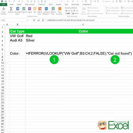
Applying the IFERROR formula is quite easy as it only has two parts (the numbers are corresponding to the image on the right hand side):
- The first part contains the original formula or value.
- The second part defines what to do in case of an error. That could be a text, a number or another formula.
Usually you would start by just creating your original formula. If you then see that it produces an error you can wrap the IFERROR formula around it.
Let’s take a closer look at the example on the picture:
=IFERROR(VLOOKUP("VW Golf",B3:B4,2,FALSE),"Car not found")In the middle, there is a VLOOKUP:
VLOOKUP("VW Golf",B3:B4,2,FALSE)This VLOOKUP searches for the keyword “VW Golf” in the cell range B3 to B4. When found, it is supposed to return the color from column C (set by the number 2). Please refer to this article for more information about the VLOOKUP formula.
The VLOOKUP is wrapped within the IFERROR formula. That means, that if the keyword can’t be found, the IFERROR formula returns the value to be “Car not found” instead of an error message. Simplified:
=IFERROR(VLOOKUP(),"Car not found")How to use the IFERROR formula on many different formulas at the same time?
Usually you can only add the IFERROR formula one by one around existing formulas. What if you’ve got to insert it on many existing formulas?
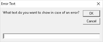
The Excel add-in ‘Professor Excel Tools’ provides an easy function for wrapping IFERROR around existing formulas: It literally just needs two clicks. Select all the formulas you want to edit and define what to do in case of an error:
- Select all existing formulas and click on the button IFERROR within the ‘Quick Cell Functions’
- You’ll see the window on the right hand side. Now you can type the value or text you want to get in case of an error. Press OK to apply.
As the trial is free, no sign-up or installation needed (just activate it within Excel) you can simply download it by clicking the button below.

This function is included in our Excel Add-In ‘Professor Excel Tools’
(No sign-up, download starts directly)

Henrik Schiffner is a freelance business consultant and software developer. He lives and works in Hamburg, Germany. Besides being an Excel enthusiast he loves photography and sports.
The IFERROR function is designed to handle errors resulting from formulas in Excel. The IFERROR function is a logical formula that is used to detect errors in formulas and returns an alternate value or performs another calculation in place of the error. If the formula nested inside the IFERROR function results in an error, the IFERROR function catches that error and returns a specified value in its place.
Excel shows errors whenever there’s something wrong with the formula or the cell it’s referencing, however, sometimes the error is unavoidable. Having an error not only makes your spreadsheet look bad but if another formula references the cell containing that error, (for instance when you sum a range of cells), it will cause another error in the second formula. So, rather than displaying an error, you can use the IFERROR function to return something else like zero, blank, or a text.
IFERROR function is an easy and elegant way to handle errors and keep your spreadsheets clean and your formulas transparent. Moreover, this function can be used in all the versions of Excel from Excel 2007. In this tutorial, we will learn what the IFERROR function is and how to use it to manage errors in Excel.
What is IFERROR Function in Excel?
The IFERROR function is a built-in function that returns a specified value if the formula nested in results in an error.
The Syntax of IFERROR function:
=IFERROR(value,value_if_error)The function has only two arguments:
value(required) – This is the value, expression, formula, or cell reference that is to be checked for errors. If the value or the result is an error it will return TRUE otherwise it will return FALSE.value_if_error(required) – This argument specifies what value to return or calculation to perform if an error is found. It could be anything a text string, a numeric value, an empty string (blank cell), another formula, expression, or calculation. If you specify a text string, you must enclose it in double quotes (” ”).
Also, if there is no error is found, it will return the usual result of the formula or expression in the value argument.
You can use the IFERROR function to detect and handle various formula errors such as the following:
- #N/A.
- #VALUE!
- #REF!
- #DIV/0!
- #NUM!
- #NAME?
- #NULL!
Most of the time, when you encounter these errors you can resolve the issue by correcting the formula. But, occasionally, these errors are inevitable and you might be expecting them. So, to deal with these errors, you can use the IFERROR function to substitute a value or function for the error.
Don’t confuse the IFERROR function with another similar error checking function, the ISERROR function which is to be used to check for errors and return simple TRUE or FALSE.
How to Use IFERROR function
Let us see how to catch errors using the IFERROR function and return different kinds of values instead of errors with examples.
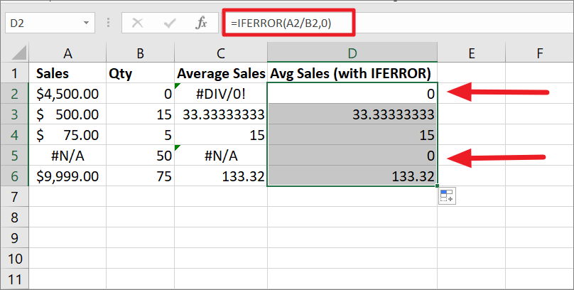
If Error, Then Return 0
If you encounter an error in your formula, you can use the IFERROR function to return ‘0’ instead of the error.
Example 1:
For instance, in the below example, we wanted to find out the average sales of different items, so we divided the Sales values in column A by the Qty (Quality) values in Column B.
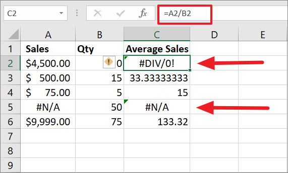
In the table, the Quantity value in B2 is 0, and the sales value in A5 is a #N/A (Not available) error. As a result, we ended up with #DIV/0! in C2 because when any number is divided by 0 (divisor), Excel throws the #DIV/0! error. And when #N/A error is divided by 50, it outputted another #N/A error in return.
With the help of the IFERROR function, we can return ‘0’ as a result instead of displaying the error codes.
To handle the errors, you can nest the formula inside the IFERROR function:
=IFERROR(A2/B2,0)In the below example, we combined the IFERROR function with the same formula and entered it in a separate column. The above formula is entered in cell D2 and copied down to the whole column using the fill handle. As you can see below, the formula returns ‘0’ as the Average sales price when it detects an error.
Example 2:
If you ignore the second argument in the IFERROR function, the formula will return ‘0’ by default.
=IFERROR(A2/B2,)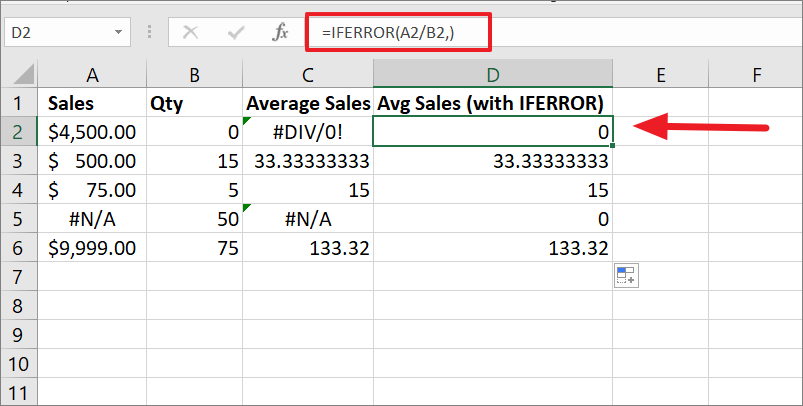
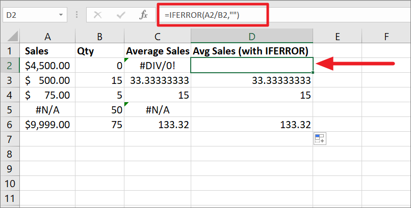
If Error, Then Return Blank
Instead of substituting 0 for errors, you specify an empty string (“) in value_if_errorargument of the IFERROR to return a blank cell if the result is an error.
Example 1:
To return a blank cell if an error is found, use the below formula:
=IFERROR(A2/B2,"")In the formula, we entered double quotations (“”) which means an empty string to return a blank cell.
Example 2:
You can also use any symbol to replace an error instead of an empty cell using the IFERROR function.
To return a symbol or a character if an error is found, use the following formula:
=IFERROR(A2/B2,"-")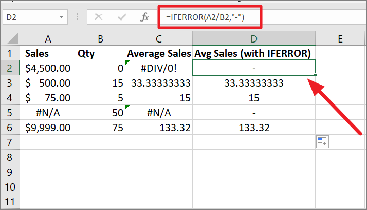
If Error, Then Show a Message/Text String
Instead of showing 0 or blank or an error, you can display your own message using the IFERROR function. When you add a text string in the second argument of the IFERROR function, make sure to enclose it in double quotes.
For example, this formula will return a message “Invalid input” instead of the error code:
=IFERROR(A2/B2,"Invalid Input")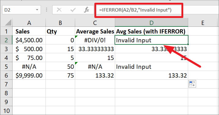
If Error, Then Perform a Calculation
With the IFERROR function, you can perform a second calculation if the first formula is evaluated to an error. You can achieve this by inputting the second formula in thevalue_if_error argument of the IFERROR.
For instance, we want to find the sales of Stock 1 by multiplying the price of an item with Stock 1 quantity. However, we have no stock of two items, so when the price is multiplied by the dash (-) symbol, we get the Value error.
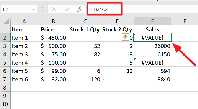
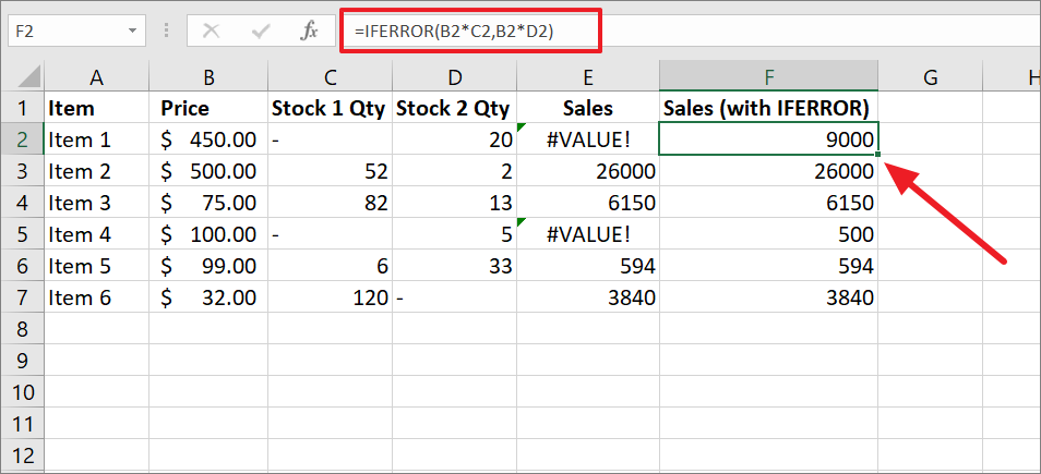
So if multiplying stock 1 quantity with price results in an error, multiply the stock 2 quantity with the price to find the sales amount of each item:
=IFERROR(B2*C2,B2*D2)In the above formula when multiplying B2 with C2 produces an error, the IFERROR function multiplies the B2 with D2 and returns the sales amount. If the first formula inside the IFERROR function didn’t result in an error, it returns that result.
IFERROR with Array Formulas
The array formula is used to perform multiple calculations in an array through a single formula. But sometimes, the Array formulas can also result in errors.
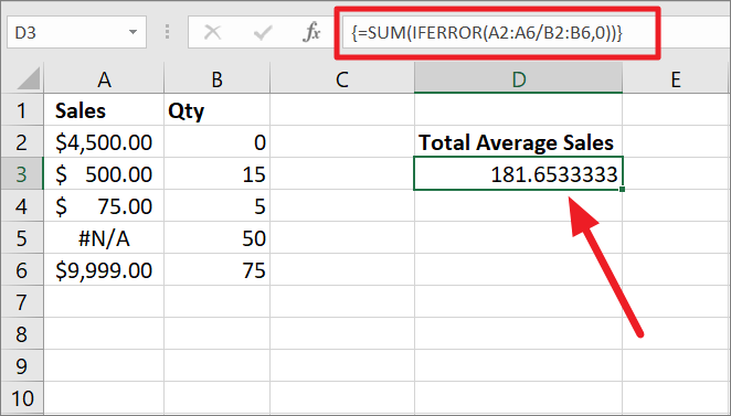
For example, we want to find the total average sales for the below table by dividing the value in column A by a value in column B in each row and summing up the results. But when we use the below array formula, it results in an error:
=SUM(A2:A6/B2:B6,0)The above formula divides each cell value in the range A2:A6 by the corresponding cell value of the range B2:B6 and returns array this array of results {#DIV/0!,33.33,15,#N/A,133.32}. Then the SUM function sums up the array of results to produce total average sales which also results in an error.
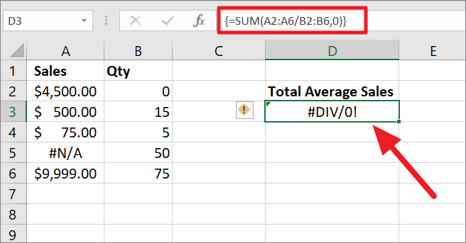
The formula divides the values in A2 by 0 and the error in A5 by the B5 which results in two errors. And when that two error values are added up with other values, we get an #DIV0! error.
To solve this problem, you just need to enclose the division operation within the IFERROR function and then wrap the IFERROR function with the SUM function:
=SUM(IFERROR(A2:A6/B2:B6,0))To execute the array formula, press Ctrl+Shift+Enter.
The IFERROR function traps all the errors and replaces them with 0, creating this array of results – {0,33.33,15,0,133.32). Then, the SUM function adds up all the results and returns ‘181.65’.
IFERROR with VLOOKUP function
The IFERROR function is often combined with the VLOOKUP function to return a custom message or text if the search value does not exist in the data set.
VLOOKUP function searches for a value in the first column of a table or a range and extracts the corresponding value from a column to the right. However, if the lookup value is not found in the table or misspelled, you will get an #N/A! error in return. So to tidy up your spreadsheet, you can use the IFERROR function to return your own message instead of the errors.
Example:
Suppose you have the below data, where you want to look up a student’s name and extract his/her score from a specific subject.
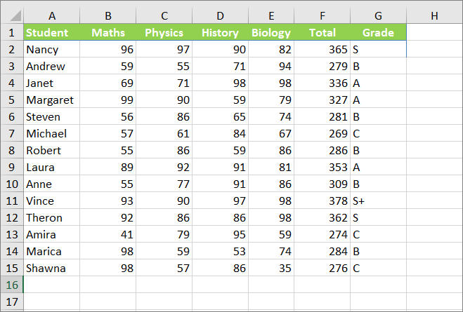
To look up a student named ‘Roger’ (J5) and return his biology score, we can use the below formula:
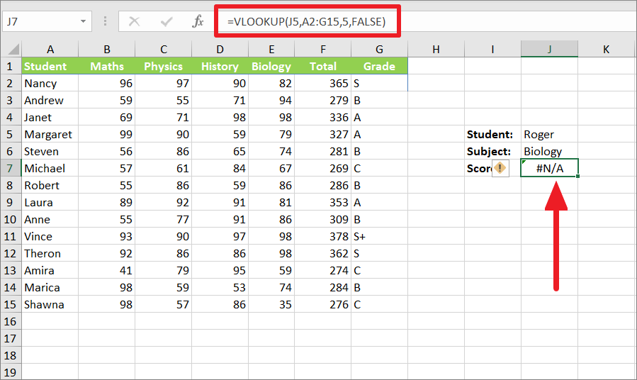
=VLOOKUP(J5,A2:G15,5,FALSE)However, the above this ends up with an error because the lookup value in cell J5 ‘Roger’ is not found in the table. Here, the first argument J5 specifies the lookup value, A2:G15 represents the range, 5 tells the function to retrieve the values from the fifth column, and FALSE means the search for the exact value.
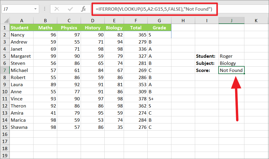
If the value is not found, you can use the IFERROR function to return a custom text string like “Not found” or “wrong input” in case of an error. To do that, you have to wrap the VLOOKUP formula as the first argument and the text string you want to return as the second argument within the IFERROR formula.
To return a custom text string, if the VLOOKUP function evaluates to an error, enter the below formula:
=IFERROR(VLOOKUP(J5,A2:G15,5,FALSE),"Not Found")The above formula looks for the value ‘Roger’ (J5) in the range ‘A2:G15’ and generates an #N/A error because the value is not found in the table. However, the IFERROR function catches that error and returns the specified string “Not Found” in its place.
If the nested VLOOKUP function does not result in an error, then the IFERROR function will simply return the standard result of the VLOOKUP function.
For example, if you change the lookup value to ‘Robert’ instead of ‘Roger’, you will get the below result:
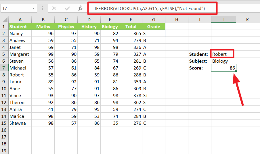
Here, we used the same formula but only changed the input value for the formula to ‘Robert’. As a result, we get the score ’86’ for the Biology subject.
IFERROR Function to Perform Sequential Vlookups
The IFERROR function can also be used to perform multiple Vlookups or sequential Vlookups based on whether the preceding lookup has resulted in an error or not.
Let’s assume you have a list of students’ scores in various subjects for Class 1 and Class 2 and you want to extract a specific student’s test score in a certain subject from class 1 using Vlookup.
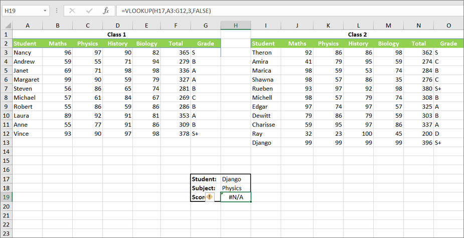
However, if the student you are searching for is not found in Class 1, you would end up with an error. So, if you nest two VLOOKUP functions (one for Class 1 and another for Class 2) as the two arguments of the IFERROR function, it performs the 2nd Vlookup operation and returns the results if the first VLOOKUP results in an error.
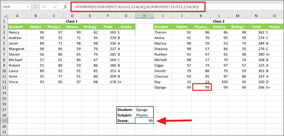
To do sequential VLOOKUPs with IFERROR, use the below formula:
=IFERROR(VLOOKUP(H17,A3:G12,3,FALSE),VLOOKUP(H17,I3:O13,3,FALSE))In the above formula, the first Vlookup function looks for the value in H17 (Django) by searching the array A3:G12 (Class 1) and if the lookup value is found, it returns the corresponding value in column 3 (Physics score). If the first VLOOKUP couldn’t find the value in Class 1, then it proceeds to the second Vlookup which searches for the values in the range I3:O13 (Class 2) and returns the Physics score for the student Django.
Nested IFERROR functions for Sequential Vlookups
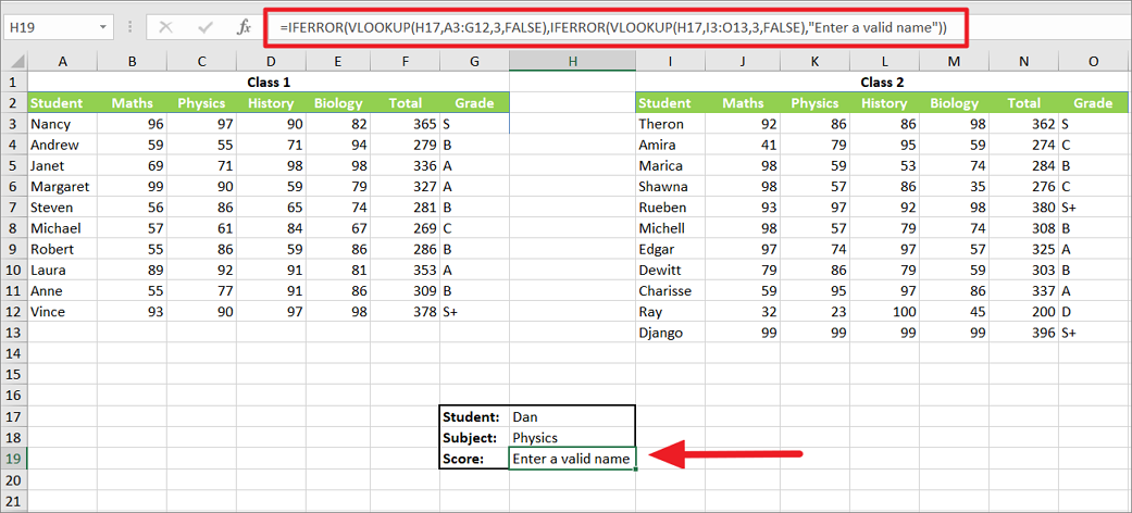
However, what if the second Vlookup is also not able to find the lookup value and fails in the above formula, then we will get an error. To prevent this, you have to create a formula to return a custom message, if the lookup value is not found in both arrays.
You need to create an IFERROR formula with the first VLOOKUP as the first argument (value) and another IFERROR function as the second argument (value_if_error). Then, nest the second VLOOKUP and a value_if_error message within the second IFERROR function:
=IFERROR(VLOOKUP(H17,A3:G12,3,FALSE),IFERROR(VLOOKUP(H17,I3:O13,3,FALSE),"Enter a valid name"))The first Vlookup inside the 1st IFERROR looks for the value ‘Dan’ in the array A3:G12 and if it fails, the second Vlookup inside the 2nd IFERROR looks for the value ‘Dan’ in the range I3:O3. If it also fails, the 2nd IFERROR returns the specified message “Enter a valid name”.
IFERROR with INDEX MATCH function
INDEX and MATCH function is a powerful lookup function more advanced than the VLOOKUP function that lets you search for a specific value in a range of cells and return a value at the specified row and column intersection.
Just like with VLOOKUP, if the INDEX MATCH function cannot find the lookup in the given range, it will return the error message. In such cases, we can use the IFERROR function to produce an alternate message or look up the value in another range by nesting the INDEX MATCH function.
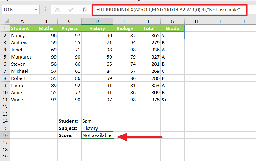
Example:
=IFERROR(INDEX(A2:G11,MATCH(D14,A2:A11,0),4),"Not available")In the above formula, the MATCH function tries to find the position of the lookup value in the range A2:A11, but the lookup value is not found in the array so the IFERROR returns the given alternate string “Not available”.
IF And IFERROR function
You can also combine the IFERROR function with the IF function to create an advanced formula and handle errors.
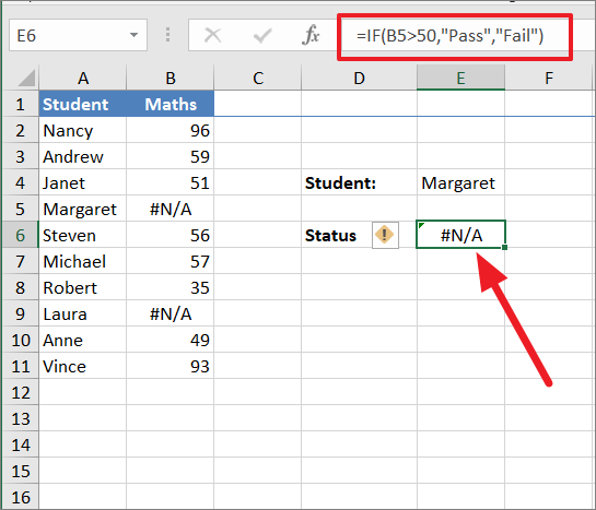
For example, we want to check whether the student Margaret is passed or failed using the IF function in the table. But Margaret’s score is not available in the table, so we get the #N/A error as the result.
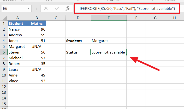
To fix this, we can use the below IF and IFERROR function combination:
=IFERROR(IF(B5>50,"Pass","Fail"),"Score not available")Here, the IF function checks whether the value in B5 is greater than 50 and returns an error. Then, the IFERROR function traps that error and displays the given alternate text string instead.
IFERROR vs. ISERROR
ISERROR function is another error-handling function that is used to check if a formula evaluates to an error or not and return TRUE or FALSE as a result. The IFERROR function returns an alternate value if a formula results in an error.
Syntax of ISERROR:
=ISERROR(value)ISERROR function (logical condition) is often used with the IF function to execute an operation or return a value if the logical condition results in an error and what to do if doesn’t result in an error.
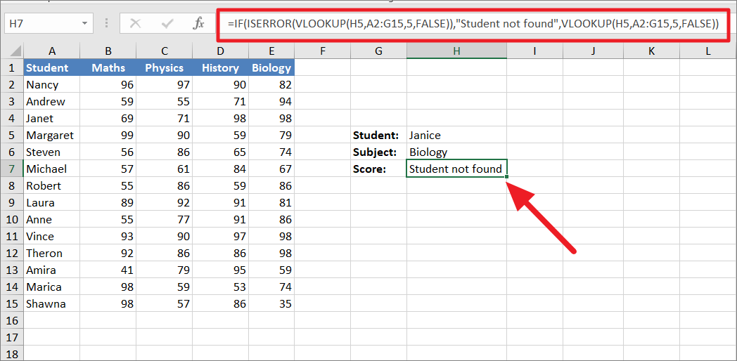
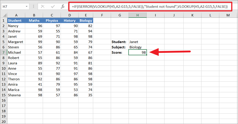
For example, we want to extract Janet’s marks in Biology using this IF ISERROR formula:
=IF(ISERROR(VLOOKUP(H5,A2:G15,5,FALSE)),"Student not found",VLOOKUP(H5,A2:G15,5,FALSE))Here, the ISERROR checks whether the nested Vlookup formula results in an error or not. If it is TRUE, then the IF function returns the message “Student not found”, otherwise it performs the Vlookup function again and returns the score ’98’.
If the lookup value (student) is not found:
or, if the student name is found:
IFNA vs. IFERROR
IFNA is another error checking function that is similar to the IFERROR that is used to catch only #N/A errors while IFERROR handles all error types. IFNA formula is useful if you only want to return a customized response for a #N/A error but not for all other errors.
Syntax of IFNA Function:
IFNA(value, value_if_na)value– the value, expression, formula, or cell reference that is to be checked for errors.value_if_na– represents what value to return or calculation to perform in case of an #N/A error. It could be anything a text string, a numeric value, empty string (blank cell), another formula, expression, or calculation.
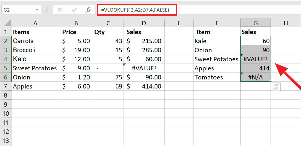
Suppose, you have the below table of sales reports and you want to pull the Sales amount of a few items from the table. To do that, we are using this simple VLOOKUP formula:
=VLOOKUP(F2,$A$2:$D$7,4,FALSE)The above formula is entered in cell G2 and the same formula is applied to the range G2:G6 using the fill handle. When we do that, we get a #VALUE! and a #N/A error for two items.
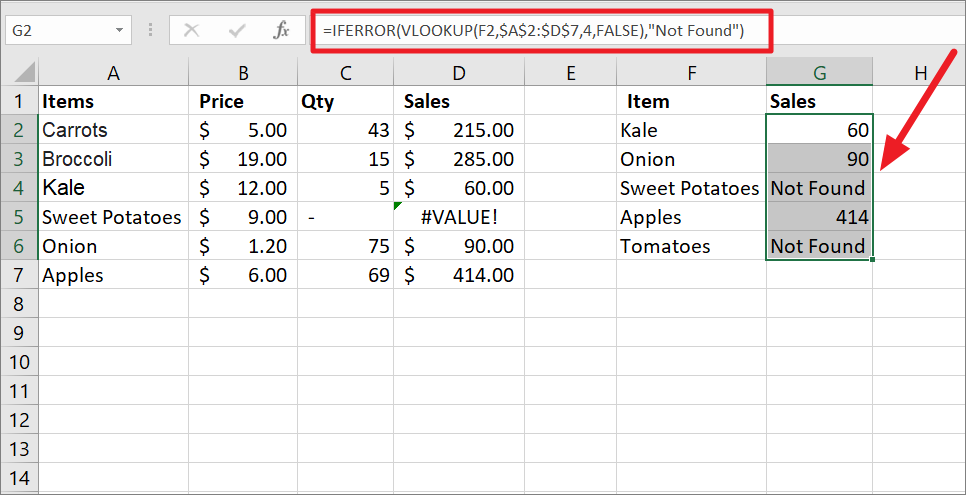
To handle these errors, you can nest the above VLOOKUP formula inside the IFERROR function:
=IFERROR(VLOOKUP(F2,$A$2:$D$7,4,FALSE),"Not Found")This IFERROR formula will handle all the errors and return the “Not Found” message whenever there’s an error is found. The above formula is applied to the whole range G2:G6.
But we don’t want that, we only want to show the “Not found” message for the items that don’t exist in the table (Tomatoes). That means, we only need to catch and handle the #N/A errors which only appear if the lookup value is not present in the lookup table. To do that, we have to nest the VLOOKUP function inside the IFNA function.
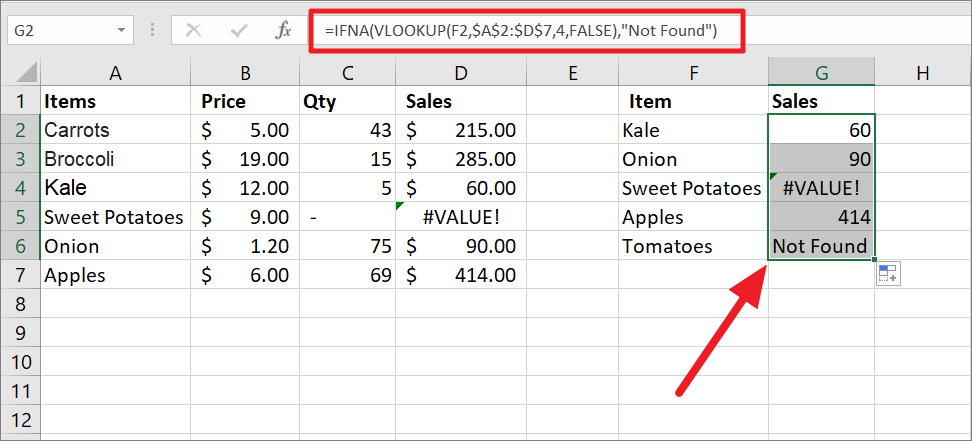
To catch only #N/A errors, use the below formula:
=IFNA(VLOOKUP(F2,$A$2:$D$7,4,FALSE),"Not Found")The above formula is applied to the range G2:G6. It checks the VLOOKUP function only for the #N/A error and returns the text “Not Found” if the item is not found in the table. As you can see below, it only catches the #N/A that occurs in cell G6 and returns the message. And it does not catch the #VALUE! error that occurs in cell G4 and displays the error as it is.
That’s it.