
Excel for Microsoft 365 Excel for Microsoft 365 for Mac Excel for the web Excel 2021 Excel 2021 for Mac Excel 2019 Excel 2019 for Mac Excel 2016 Excel 2016 for Mac Excel 2013 Excel 2010 Excel 2007 Excel for Mac 2011 More…Less
Array formulas are powerful formulas that enable you to perform complex calculations that often can’t be done with standard worksheet functions. They are also referred to as «Ctrl-Shift-Enter» or «CSE» formulas, because you need to press Ctrl+Shift+Enter to enter them. You can use array formulas to do the seemingly impossible, such as
-
Count the number of characters in a range of cells.
-
Sum numbers that meet certain conditions, such as the lowest values in a range or numbers that fall between an upper and lower boundary.
-
Sum every nth value in a range of values.
Excel provides two types of array formulas: Array formulas that perform several calculations to generate a single result and array formulas that calculate multiple results. Some worksheet functions return arrays of values, or require an array of values as an argument. For more information, see Guidelines and examples of array formulas.
Note: If you have a current version of Microsoft 365, then you can simply enter the formula in the top-left-cell of the output range, then press ENTER to confirm the formula as a dynamic array formula. Otherwise, the formula must be entered as a legacy array formula by first selecting the output range, entering the formula in the top-left-cell of the output range, and then pressing CTRL+SHIFT+ENTER to confirm it. Excel inserts curly brackets at the beginning and end of the formula for you. For more information on array formulas, see Guidelines and examples of array formulas.
This type of array formula can simplify a worksheet model by replacing several different formulas with a single array formula.
-
Click the cell in which you want to enter the array formula.
-
Enter the formula that you want to use.
Array formulas use standard formula syntax. They all begin with an equal sign (=), and you can use any of the built-in Excel functions in your array formulas.
For example, this formula calculates the total value of an array of stock prices and shares, and places the result in the cell next to «Total Value.»

The formula first multiplies the shares (cells B2 – F2) by their prices (cells B3 – F3), and then adds those results to create a grand total of 35,525. This is an example of a single-cell array formula because the formula lives in just one cell.
-
Press Enter (if you have a current Microsoft 365 Subscription); otherwise press Ctrl+Shift+Enter.
When you press Ctrl+Shift+Enter, Excel automatically inserts the formula between { } (a pair of opening and closing braces).
Note: If you have a current version of Microsoft 365, then you can simply enter the formula in the top-left-cell of the output range, then press ENTER to confirm the formula as a dynamic array formula. Otherwise, the formula must be entered as a legacy array formula by first selecting the output range, entering the formula in the top-left-cell of the output range, and then pressing CTRL+SHIFT+ENTER to confirm it. Excel inserts curly brackets at the beginning and end of the formula for you. For more information on array formulas, see Guidelines and examples of array formulas.
To calculate multiple results by using an array formula, enter the array into a range of cells that has the exact same number of rows and columns that you’ll use in the array arguments.
-
Select the range of cells in which you want to enter the array formula.
-
Enter the formula that you want to use.
Array formulas use standard formula syntax. They all begin with an equal sign (=), and you can use any of the built-in Excel functions in your array formulas.
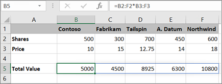
In the following example, the formula multiples shares by price in each column, and the formula lives in the selected cells in row 5.
-
Press Enter (if you have a current Microsoft 365 Subscription); otherwise press Ctrl+Shift+Enter.
When you press Ctrl+Shift+Enter, Excel automatically inserts the formula between { } (a pair of opening and closing braces).
Note: If you have a current version of Microsoft 365, then you can simply enter the formula in the top-left-cell of the output range, then press ENTER to confirm the formula as a dynamic array formula. Otherwise, the formula must be entered as a legacy array formula by first selecting the output range, entering the formula in the top-left-cell of the output range, and then pressing CTRL+SHIFT+ENTER to confirm it. Excel inserts curly brackets at the beginning and end of the formula for you. For more information on array formulas, see Guidelines and examples of array formulas.
If you need to include new data in your array formula, see Expand an array formula. You can also try:
-
Rules for changing array formulas (they can be finicky)
-
Delete an array formula (you press Ctrl+Shift+Enter there, too)
-
Use array constants in array formulas (they can be handy)
-
Name an array constant (they can make constants easier to use)
If you want to play around with array constants before you try them out with your own data, you can use the sample data here.
The workbook below shows examples of array formulas. To best work with the examples, you should download the workbook to your computer by clicking the Excel icon in the lower-right corner, and then open it in the Excel desktop program.
Copy the table below and paste it into Excel in cell A1. Be sure to select cells E2:E11, enter the formula =C2:C11*D2:D11, and then press Ctrl+Shift+Enter to make it an array formula.
|
Salesperson |
Car Type |
Number Sold |
Unit Price |
Total Sales |
|---|---|---|---|---|
|
Barnhill |
Sedan |
5 |
2200 |
=C2:C11*D2:D11 |
|
Coupe |
4 |
1800 |
||
|
Ingle |
Sedan |
6 |
2300 |
|
|
Coupe |
8 |
1700 |
||
|
Jordan |
Sedan |
3 |
2000 |
|
|
Coupe |
1 |
1600 |
||
|
Pica |
Sedan |
9 |
2150 |
|
|
Coupe |
5 |
1950 |
||
|
Sanchez |
Sedan |
6 |
2250 |
|
|
Coupe |
8 |
2000 |
Create a multi-cell array formula
-
In the sample workbook, select cells E2 through E11. These cells will contain your results.
You always select the cell or cells that will contain your results before you enter the formula.
And by always, we mean 100-percent of the time.
-
Enter this formula. To enter it in a cell, just start typing (press the equal sign) and the formula appears in the last cell you selected. You can also enter the formula in the formula bar:
=C2:C11*D2:D11
-
Press Ctrl+Shift+Enter.
Create a single-cell array formula
-
In the sample workbook, click cell B13.
-
Enter this formula using either method from step 2 above:
=SUM(C2:C11*D2:D11)
-
Press Ctrl+Shift+Enter.
The formula multiplies the values in the cell ranges C2:C11 and D2:D11, then adds the results to calculate a grand total.
In Excel for the web, you can view array formulas if the workbook you open already has them. But you won’t be able to create an array formula in this version of Excel by pressing Ctrl+Shift+Enter, which inserts the formula between a pair of opening and closing braces({ }). Manually entering these braces won’t turn the formula into an array formula either.
If you have the Excel desktop application, you can use the Open in Excel button to open the workbook and create an array formula.
Need more help?
You can always ask an expert in the Excel Tech Community or get support in the Answers community.
Need more help?
Содержание
- Array formulas
- Want more?
- Create an array formula
- Array
- Related terminology
- Example
- Array syntax
- Delimiters in other languages
- Arrays in formulas
- Array formulas
- Dynamic arrays
- Working with Excel array formula examples
- Types of Excel functions
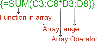
- Array formulas syntax
- Working functions with Excel array
Array formulas

Create array formulas, often called Ctrl+Shift+Enter or CSE formulas, to perform calculations that generate single or multiple results. Watch this video to learn more.
Why use array formulas?
Array formulas are often referred to as CSE (Ctrl+Shift+Enter) formulas because instead of just pressing Enter, you press Ctrl+Shift+Enter to complete the formula.
If you have an experience using formulas in Excel, you know that you can perform some fairly sophisticated operations. For example, you can calculate the total cost of a loan over any given number of years. You can use array formulas to do complex tasks, such as:
Count the number of characters that are contained in a range of cells.
Sum only numbers that meet certain conditions, such as the lowest values in a range or numbers that fall between an upper and lower boundary.
Sum every nth value in a range of values.
Enter an array formula
Select the cells where you want to see your results.
Enter your formula.
Press Ctrl+Shift+Enter. Excel fills each of the cells you selected with the result.
Want more?
You want to calculate the total of a large range of cells, such as the value of these Stocks.
You could type = sign, B2 (the number of Contoso shares), asterisk to multiply, B3, the share price, the + sign to add, C2, asterisk, C3, and so on.
But it would take forever with a large series, and it would be easy to make a mistake, and not notice it.
An easier way? Use an array formula. An array is a series of data in a row, column, or a combination of rows and columns.
You have probably used them before. B2:F2 is an array, also commonly referred to as a range of cells.
An array formula performs calculations on the data in one or more arrays, returning either a single or multiple results.
With an array formula, you type = sign, SUM, opening parenthesis, select the cells in the Shares row (this is the first array in the array formula), then an asterisk to multiply, select the cells in the Price row (this is the second array in the array formula).
And this is the key difference when you enter an array formula, you press Ctrl+Shift+Enter, not just Enter.
If you press just Enter, you’ll get either an incorrect value, if the regular function is valid, or a value error, if it is not.
I didn’t type a closing parenthesis in the formula, pressing Ctrl+Shift+Enter does this for you.
The array formula multiplies each cell in the Shares row by the respective cell in the Price row and then sums, or adds these and returns the total of $14,421.87.
In the Formula Bar, the formula is enclosed in braces, < >, meaning that it is an array formula.
This is automatically done when you press Ctrl+Shift+Enter. Don’t type these braces. If you do, Excel will interpret your formula as text, not as a formula.
Up next: Use SUM, AVERAGE, and MAX in array formulas.
Источник
Create an array formula
Array formulas are powerful formulas that enable you to perform complex calculations that often can’t be done with standard worksheet functions. They are also referred to as «Ctrl-Shift-Enter» or «CSE» formulas, because you need to press Ctrl+Shift+Enter to enter them. You can use array formulas to do the seemingly impossible, such as
Count the number of characters in a range of cells.
Sum numbers that meet certain conditions, such as the lowest values in a range or numbers that fall between an upper and lower boundary.
Sum every nth value in a range of values.
Excel provides two types of array formulas: Array formulas that perform several calculations to generate a single result and array formulas that calculate multiple results. Some worksheet functions return arrays of values, or require an array of values as an argument. For more information, see Guidelines and examples of array formulas.
Note: If you have a current version of Microsoft 365, then you can simply enter the formula in the top-left-cell of the output range, then press ENTER to confirm the formula as a dynamic array formula. Otherwise, the formula must be entered as a legacy array formula by first selecting the output range, entering the formula in the top-left-cell of the output range, and then pressing CTRL+SHIFT+ENTER to confirm it. Excel inserts curly brackets at the beginning and end of the formula for you. For more information on array formulas, see Guidelines and examples of array formulas.
This type of array formula can simplify a worksheet model by replacing several different formulas with a single array formula.
Click the cell in which you want to enter the array formula.
Enter the formula that you want to use.
Array formulas use standard formula syntax. They all begin with an equal sign (=), and you can use any of the built-in Excel functions in your array formulas.
For example, this formula calculates the total value of an array of stock prices and shares, and places the result in the cell next to «Total Value.»
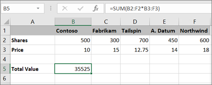
The formula first multiplies the shares (cells B2 – F2) by their prices (cells B3 – F3), and then adds those results to create a grand total of 35,525. This is an example of a single-cell array formula because the formula lives in just one cell.
Press Enter (if you have a current Microsoft 365 Subscription); otherwise press Ctrl+Shift+Enter.
When you press Ctrl+Shift+Enter, Excel automatically inserts the formula between (a pair of opening and closing braces).
Note: If you have a current version of Microsoft 365, then you can simply enter the formula in the top-left-cell of the output range, then press ENTER to confirm the formula as a dynamic array formula. Otherwise, the formula must be entered as a legacy array formula by first selecting the output range, entering the formula in the top-left-cell of the output range, and then pressing CTRL+SHIFT+ENTER to confirm it. Excel inserts curly brackets at the beginning and end of the formula for you. For more information on array formulas, see Guidelines and examples of array formulas.
To calculate multiple results by using an array formula, enter the array into a range of cells that has the exact same number of rows and columns that you’ll use in the array arguments.
Select the range of cells in which you want to enter the array formula.
Enter the formula that you want to use.
Array formulas use standard formula syntax. They all begin with an equal sign (=), and you can use any of the built-in Excel functions in your array formulas.
In the following example, the formula multiples shares by price in each column, and the formula lives in the selected cells in row 5.
Press Enter (if you have a current Microsoft 365 Subscription); otherwise press Ctrl+Shift+Enter.
When you press Ctrl+Shift+Enter, Excel automatically inserts the formula between (a pair of opening and closing braces).
Note: If you have a current version of Microsoft 365, then you can simply enter the formula in the top-left-cell of the output range, then press ENTER to confirm the formula as a dynamic array formula. Otherwise, the formula must be entered as a legacy array formula by first selecting the output range, entering the formula in the top-left-cell of the output range, and then pressing CTRL+SHIFT+ENTER to confirm it. Excel inserts curly brackets at the beginning and end of the formula for you. For more information on array formulas, see Guidelines and examples of array formulas.
If you need to include new data in your array formula, see Expand an array formula. You can also try:
Delete an array formula (you press Ctrl+Shift+Enter there, too)
Name an array constant (they can make constants easier to use)
Источник
Array

An array in Excel is a structure that holds a collection of values. Arrays can be mapped perfectly to ranges in a spreadsheet, which is why they are so important in Excel. An array can be thought of as a row of values, a column of values, or a combination of rows and columns with values. All cell references like A1:A5 and C1:F5 have underlying arrays, though the array structure is invisible in most contexts.
Example
In the example above, the three ranges map to arrays in a «row by column» scheme like this:
If we display the values in these ranges as arrays, we have:
Notice arrays must represent a rectangular structure.
Array syntax
All arrays in Excel are wrapped in curly brackets <> and the delimiters between array elements indicate rows and/or columns. In the US version of Excel, a comma (,) separates columns and a semicolon (;) separates rows. For example, both arrays below contain numbers 1-3, but one is horizontal and one is vertical:
Text values in an array appear in double quotes («») like this:
To «see» the array associated with a range, start a formula with an equal sign (=) and select the range. Then use the F9 key to inspect the underlying array. You can also use the ARRAYTOTEXT function to show how columns and rows are represented. Set format to 1 (strict) to see the complete array.
Delimiters in other languages
In other language versions of Excel, the delimiters for rows and column can vary. For example, the Spanish version of Excel uses a backslash () for columns and a semicolon (;) for rows:
Arrays in formulas
Since arrays map directly to ranges, all formulas work with arrays in some way, though it isn’t always obvious. A simple example is a formula that uses the SUM function to sum the range A1:A5, which contains 10,15,20,25,30. Inside SUM, the range resolves to an array of values. SUM then sums all values in the array and returns a single result of 100:
Note: you can use the F9 key to «see» arrays in your Excel formulas. See this video for a demo on using F9 to debug.
Array formulas
Array formulas involve an operation that delivers an array of results. For example, here is a simple array formula that returns the total count of characters in the range A1:A5:
Inside the LEN function, A1:A5 is expanded to an array of values. The LEN function then generates a character count for each value and returns an array of 5 results. The SUM function then returns the sum of all items in the array.
Dynamic arrays
With the introduction of Dynamic Array formulas in Excel, arrays have become more important, since it is easier than ever to write formulas that work with multiple results at the same time.
Источник
Working with Excel array formula examples
The array of Excel functions allows you to solve complex tasks in automatically at the same time. We cannot complete the same tasks through the usual functions.
In fact, this is a group of functions that simultaneously process a group of data and immediately produce a result. Let’s consider in detail work with arrays of functions in Excel.
Types of Excel functions
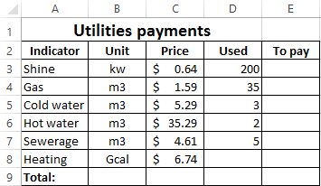
Array is a data grouped together. In this case, the group is an array of functions in Excel. Any table that we compose and fill in Excel can be called an array. Example:
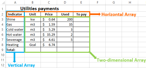
Depending on the location of the elements, the arrays are distinguished:
- One-dimensional (data is in ONE line or in ONE column);
- Two-dimensional (SEVERAL lines and columns, matrix).
One-dimensional arrays are:
- Horizontal (data in a row);
- Vertical (data in a column).
Note. Two-dimensional Excel arrays can take several sheets at once (these are hundreds and thousands of data).
Array formula allows you to process data from this array. It can return one value or result in an array (set) of values.
With the help of array formulas it is real to:
- Count the number of characters in a certain range;
- Summarize only those numbers that correspond to the given condition;
- Summarize all n values in a certain range.
When we use array formulas, Excel takes into account the range of values not as individual cells, but as a single data block.
Array formulas syntax
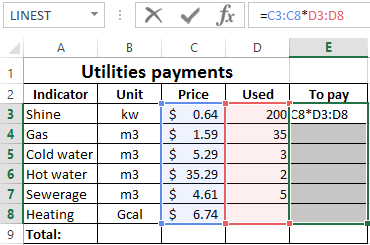
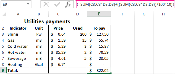
We use the formula of an array with a range of cells and with a separate cell. In the first case, we find the subtotals for the «To pay» «» column. In the second — the total amount of utility payments.
- We select the range E3: E8.
- Enter the following formula in the formula row: = C3: C8 * D3: D8.
- Press the keys simultaneously: Ctrl + Shift + Enter. The subtotals are calculated:
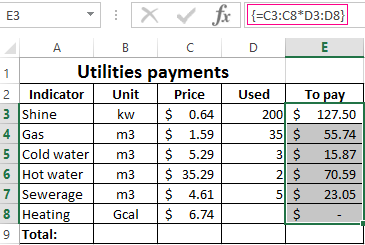
The formula after pressing Ctrl + Shift + Enter was in curly brackets. It was automatically inserted into each cell of the selected range.
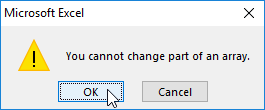
If you try to change the data in any cell in the «To pay» column, nothing happens. The formula in the array protects range values from changes. A corresponding entry appears on the screen:
Consider other examples of using the functions of an Excel array — calculate the total amount of utility payments using a single formula.
- Select the cell E9 (opposite the «Total»).
- We introduce a formula of the form:
- Press the key combination: Ctrl + Shift + Enter. Result:
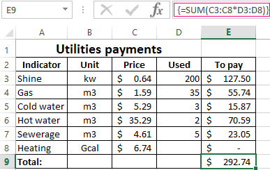
The formula of the array in this case replaced two simple formulas. This is a shortened version, which contains all the necessary information for solving a complex problem.
Arguments for a function are one-dimensional arrays. The formula looks at each of them individually, performs user-defined operations, and generates a single result.
Consider the syntax:
Working functions with Excel array
Let’s guess that it is planned to increase utility payments in 10% the next month. If we introduce the usual formula for the total is =SUM((C3:C8*D3:D8)+10%), then we are unlikely to get the expected result. We need each argument to increase in 10%. For the program to understand this, we use the function as an array.
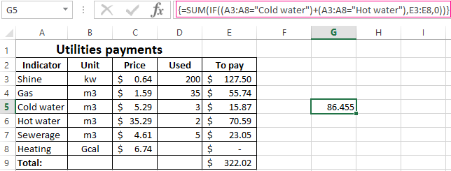
- Let’s have a look how the «И» «AND» operator works in the array function. We need to find out how much we pay for the water, hot and cold. Function: The total is 86.46$.
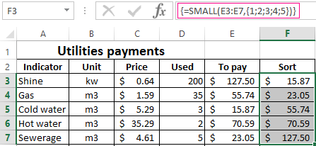
- The Sort functions in the array formula. Sort the amounts to be paid in ascending order. For the sorted data list, create a range. Let’s select it (F3:F7). In the formula bar, we enter Press Ctrl + Shift + Enter.
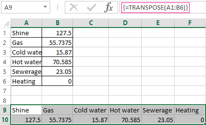
- The transported matrix. There is a special Excel function for working with two-dimensional arrays. The «ТРАНСП» function returns several values at once. It converts a horizontal matrix to a vertical matrix and vice versa. Select the range of cells where the number of rows equals to the number of columns in the table with the original data. And the number of columns equals to the number of rows in the source array. Select range A9:F10. We introduce the formula: Press Ctrl + Shift + Enter. This results in an «inverted» data set.
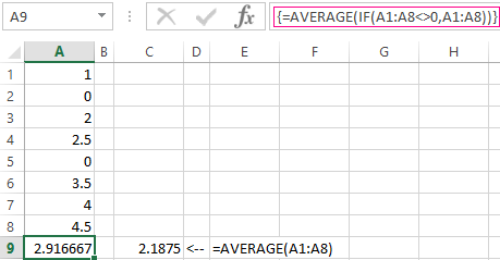
- Search for the average without taking into account zeros. If we use the standard «AVERAGE» function, we get «0» as a result. And it will be correct. Therefore, we insert an additional condition into the formula:
0,A1:A8))’ >
A common mistake when working with arrays of functions is NOT to press the code combination «Ctrl + Shift + Enter» (never forget this key combination). This is the most important thing to remember when processing large amounts of information. Correctly entered function performs the most complicated tasks.
Источник
Asked by: Hermann Hayes DVM
Score: 4.5/5
(39 votes)
Enter an array formula
- Select the cells where you want to see your results.
- Enter your formula.
- Press Ctrl+Shift+Enter. Excel fills each of the cells you selected with the result.
How do you create an array in Excel?
Creating an Array Formula
- You need to click on cell in which you want to enter the array formula.
- Begin the array formula with the equal sign and follow the standard formula syntax and use mathematical operators or built in functions in Excel formula, as required. …
- Press Ctrl+Shift+Enter to produce the desired result.
How does array formula work in Excel?
In Excel, an Array Formula allows you to do powerful calculations on one or more value sets. The result may fit in a single cell or it may be an array. An array is just a list or range of values, but an Array Formula is a special type of formula that must be entered by pressing Ctrl+Shift+Enter.
How do I array multiple cells in Excel?
Multi-cell array formulas have unique characteristics: All cells display the same formula (relative references don’t change)
…
Steps to enter a multi-cell array formula
- Select multiple cells (cells that will contain the formula)
- Enter an array formula in the formula bar.
- Confirm formula with Control + Shift + Enter.
What does {} do in Excel?
Entering An Array Formula
Press CTRL+SHIFT+ENTER to confirm this formula (instead of just pressing ENTER). This will produce curly brackets {} around the formula. These curly brackets are how Excel recognises an array formula. They cannot be entered manually, they must be produced by pressing CTRL+SHIFT+ENTER.
30 related questions found
What is Excel array?
An array in Excel is a structure that holds a collection of values. Arrays can be mapped perfectly to ranges in a spreadsheet, which is why they are so important in Excel. An array can be thought of as a row of values, a column of values, or a combination of rows and columns with values.
What does a $1 mean in Excel?
A$1. Allows the column reference to change, but not the row reference. $A$1. Allows neither the column nor the row reference to change. There is a shortcut for placing absolute cell references in your formulas!
How do I resize an array in Excel?
Here’s what you need to do.
- Select the range of cells that contains your current array formula, plus the empty cells next to the new data.
- Press F2. Now you can edit the formula.
- Replace the old range of data cells with the new one. …
- Press Ctrl+Shift+Enter.
What is array formula?
An array formula is a formula that can perform multiple calculations on one or more items in an array. You can think of an array as a row or column of values, or a combination of rows and columns of values. Array formulas can return either multiple results, or a single result.
What is array give the example?
An array is a data structure that contains a group of elements. Typically these elements are all of the same data type, such as an integer or string. … For example, a search engine may use an array to store Web pages found in a search performed by the user.
What is an array value?
An array is a table (consisting of rows and columns) of values. If you want to group the values of your cells together in a particular order, you can use arrays in your spreadsheet. … For example, IMPORTRANGE returns an array of values by importing the specified range from another spreadsheet.
What is Ctrl enter in Excel?
If we hold the Ctrl key while pressing Enter, the selection will NOT move to the next cell. Instead, the cell that we just edited will remain selected. The cell we are editing is referred to as the active cell. So, Ctrl+Enter keeps the selection on the active cell after entering data or a formula.
How do you create an array?
An array is a sequence of values; the values in the array are called elements. You can make an array of int s, double s, or any other type, but all the values in an array must have the same type. To create an array, you have to declare a variable with an array type and then create the array itself.
How do you write a Countif criteria?
Use COUNTIF, one of the statistical functions, to count the number of cells that meet a criterion; for example, to count the number of times a particular city appears in a customer list. In its simplest form, COUNTIF says: =COUNTIF(Where do you want to look?, What do you want to look for?)
Are array formulas faster?
But if you want to use them for the same task, array formulas can be a bit faster, but a bit more difficult for editing. For example, you can expand range of array formula by mouse, but you cannot shrink it etc. As a side effect, you can’t easily overwrite array formula ranges.
How do you use an array?
Obtaining an array is a two-step process. First, you must declare a variable of the desired array type. Second, you must allocate the memory that will hold the array, using new, and assign it to the array variable. Thus, in Java all arrays are dynamically allocated.
What are dynamic arrays in Excel?
Dynamic Arrays are resizable arrays that calculate automatically and return values into multiple cells based on a formula entered in a single cell. Through over 30 years of history, Microsoft Excel has undergone many changes, but one thing remained constant — one formula, one cell.
How do you fill down an array in Excel?
Use ‘Edit’ > ‘Fill’ > ‘Down’ (default shortcut: Ctrl+D) after selecting the range to fill. You may also press Ctrl in addition to dragging the «little square».
How do you autofill an array formula in Excel?
Enter an array formula
Enter your formula. Press Ctrl+Shift+Enter. Excel fills each of the cells you selected with the result.
How do you shrink an array?
An array cannot be resized dynamically in Java.
- One approach is to use java. util. ArrayList(or java. util. Vector) instead of a native array.
- Another approach is to re-allocate an array with a different size and copy the contents of the old array to the new array.
WHAT IS A in Excel formula?
COUNT(A:A) – Counts all values that are numerical in A column. However, you must adjust the range inside the formula to count rows. COUNT(A1:C1) – Now it can count rows. Image: CFI’s Excel Courses.
What does F9 do in Excel?
F9: Calculates all worksheets in all open workbooks. Shift+F9: Calculates the active worksheet. Ctrl+Alt+F9: Calculates all worksheets in all open workbooks, regardless of whether they have changed since the last calculation.
What does a $2 mean in Excel?
The $ tells Excel to NOT interpret the cell reference literally, but to always use exactly this location. For example, if you were to copy this formula down the column you would always see $A$2 and A$2. If your original formula were: =WEEKDAY(A2 + VALUE(A2)-1,1) = 7.
What is difference between range and array?
An array is an object that’s a collection of arbitrary elements. A range is an object that has a «start» and an «end», and knows how to move from the start to the end without having to enumerate all the elements in between.
What is a table array?
And Table Array is the combination of two or more than two tables which has data and values linked and related to one another. Although headers may be a quite different relation of those data with each other will be seen.
In Excel, an Array Formula allows you to do powerful calculations on one or more value sets. The result may fit in a single cell or it may be an array. An array is just a list or range of values, but an Array Formula is a special type of formula that must be entered by pressing Ctrl+Shift+Enter. The formula bar will show the formula surrounded by curly brackets {=…}.
Array formulas are frequently used for data analysis, conditional sums and lookups, linear algebra, matrix math and manipulation, and much more. A new Excel user might come across array formulas in other people’s spreadsheets, but creating array formulas is typically an intermediate-to-advanced topic.
Download the Example File (ArrayFormulas.xlsx)
Topics and Examples in This Article:
- Entering an Array Formula
- Using Array Constants
- A Simple Array Formula Example
- Entering a Multi-Cell Array Formula
- Nested IF Array Formulas
- COUNTIF Alternative: SUM-Boolean Array Formulas
- Multi-Criteria Boolean Array Formulas
- Sequential Number Arrays (1,2,3,…)
- Formulas for Matrices: MUNIT, MMULT, TRANSPOSE, etc.
- Other Array Formula Examples
Watch the Intro Video
Entering and Identifying an Array Formula
- When using an Array Formula, you press Ctrl+Shift+Enter instead of just Enter after entering or editing the formula. This is why array formulas are often called CSE formulas.
- An Array Formula will show curly brackets or braces around the formula in the Formula Bar like this: {=SUM(A1:A5*B1:B5)}
- Array Constants (arrays «hard-coded» into formulas) are enclosed in braces { } and use commas to separate columns, and semi-colons to separate rows, like this 2×3 array: {1, 1, 1; 2, 2, 2}
- If an Array Formula returns more than one value (a multi-cell array formula), first select a range of cells equal to size of the returned array, then enter your formula.
- To select all the cells within a multi-cell array: Press F5 > Special > Current Array.
! Every time you edit an Array Formula, you must remember to press Ctrl+Shift+Enter afterward. If you forget to, the formula may return an error without you realizing it.
NOTE Google Sheets uses the ARRAYFORMULA function instead of showing the formula surrounded by braces. It is not necessary to press Ctrl+Shift+Enter in Google Sheets, but if you do, ARRAYFORMULA( is added to the beginning of the formula.
Using Array Constants in Formulas
Many functions allow you use array constants like {1,2,6,12} as arguments within formulas. An example that I often use in my yearly calendar templates returns the weekday abbreviation for a given date. The nice thing about this formula is that you can choose whether to display a single character or two characters.
=INDEX({"Su";"M";"Tu";"W";"Th";"F";"Sa"},WEEKDAY(theDate,1))
This formula is not technically an Array Formula because you don’t enter it using Ctrl+Shift+Enter. Using a hard-coded array within a formula does not necessarily require using Ctrl+Shift+Enter.
TIP If you are going to use the array constant in multiple formulas, you may want to first create a Named Constant. Go to Formulas > Name Manager > New Name, enter a descriptive name like payment_frequency and enter ={1,2,6,12} into the Refers To field. You can use the name within your formulas. If you ever want to change the values within that array constant, you only need to change it one place (within the Name Manager).
A Simple Array Formula Example
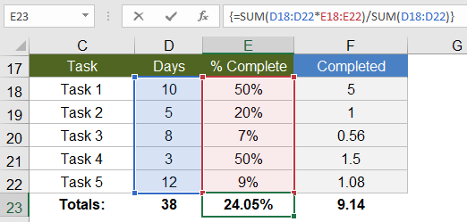
To start out, I will show how an array formula works using a very basic example. Let’s say that I have a list of tasks, the number of days each of those tasks will take, and a column for the percent complete. I want to know the total number of days that have been completed.
Without an array formula, you would create another column called «Completed» and multiply the number of days by the % complete, and copy the formula down. Then I would use SUM to total the number of days completed, like the image below:
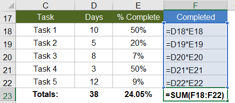
With an array formula, you can do essentially the same thing without having to create the extra column. Within a single cell, you can calculate the total days completed as =SUM(D18:D22*E18:E22), remembering to press Ctrl+Shift+Enter because it is an array formula.
{ =SUM(D18:D22*E18:E22) }

Evaluation Steps
Step 1: =SUM( {10;5;8;3;12} * {0.5;0.2;0.07;0.5;0.09} )
Step 2: =SUM( {10*0.5;5*0.2;8*0.7;3*0.5;12*0.09} )
Step 3: =SUM( {5;1;0.56;1.5;1.08} )
Step 4: =9.14
In this and other examples, I’ve shown the evaluation steps below the formula so that you can see how the formula works. You don’t actually type the curly brackets { }, but in this article I will surround all array formulas with brackets to indicate that they are entered as CSE formulas.
In the evaluation steps shown in the above example, you’ll see that Excel is multiplying each element of the first array by the corresponding element in the second array, and then SUM adds the results.
NOTE It turns out that this particular example can be used to show how the SUMPRODUCT function works, but the SUMPRODUCT function deserves its own article.
To take this example just a bit further, if all we wanted to know was the Total Percent Complete for the entire project, we can divide the total days completed (9.14) by the total days (38) all within a single array formula, and we don’t need column F at all (as shown in the image below).
This example is an example of a single-cell array formula, meaning that the formula is entered into a single cell.
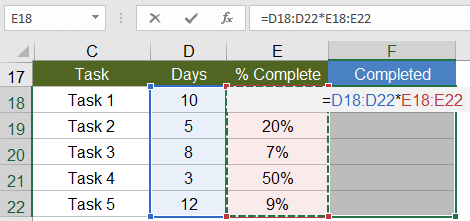
Entering a Multi-Cell Array Formula
Whenever your array formula returns more than one value, if you want to display more than just the first value, you need to select the range of cells that will contain the resulting array before entering your formula. Doing this will result in a multi-cell array formula, meaning that the result of the formula is a multi-cell array.
Using the same example as above, we could use an array formula in the Completed column to calculate Days * Percent Complete. First, select cells F18:F22, then press = and enter the formula, followed by Ctrl+Shift+Enter (CSE). The image below is what it will look like just before you press CSE.
You can edit a multi-cell array formula by selecting any of the cells in the array and then updating the formula and pressing Ctrl+Shift+Enter when you are done. However, you can’t use this technique to modify the size of the array.
«You can’t change part of an array» — This is the warning or error you will get if you try to insert rows or columns or change individual cells within a multi-cell array.
Using multi-cell array formulas can make it more difficult to customize a spreadsheet because to change the size of the array requires that you (1) delete the formula (after selecting all the cells of the array), (2) select the new range of cells, and (3) re-enter the array formula. TIP: Make sure to copy your original formula before deleting it. Then, when you re-enter the formula, you can paste it and modify the ranges.
Nested IF Array Formulas
A nested IF array formula can be very powerful and is probably one of the more common uses for array formulas in Excel. Although Excel provides the SUMIF and COUNTIF and AVERAGEIF functions, they don’t allow as much freedom as a nested IF array formula.
MAX-IF Array Formula
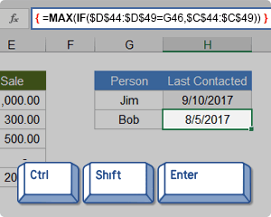
Older versions of Excel do not have the MAXIFS or MINIFS functions, so let’s create our own MAX-IF formula. When we use hyphens to name a formula, it usually means that we’re nesting the functions (IF within MAX in this case).
Let’s say that I have the following contact and sales log and I want a formula that will tell me when I last contacted Bob (cell H51).
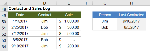
Using MAX on the date range will give me that latest date (9/10/2017), but I only want to include the rows where the contact is Bob. So, I’ll use the MAX-IF array formula:
{ =MAX(IF(contact_range="Bob",date_range)) }

Evaluation Steps
Step 1: =MAX(IF({"Jim";"Bob";"Jim";"Bob";"Jim"}="Bob", date_range ))
Step 2: =MAX(IF({FALSE;TRUE;FALSE;TRUE;FALSE}, date_range ))
Step 3: =MAX( {FALSE,2/25/2017,FALSE,8/5/2017,FALSE} )
Step 4: =8/5/2017
LARGE-IF Array Formula
The LARGE and SMALL functions come in handy when you want to find the value that is perhaps the 2nd largest or 2nd smallest.
The following function will return the second largest sale where the contact is Jim.
{ =LARGE(IF(contact_range="Jim",sale_range),2) }
SMALL-IF Array Formula
This function returns the second smallest sale where the contact is Jim.
{ =SMALL(IF(contact_range="Jim",date_range),2) }
The LARGE and SMALL functions can be used for sorting arrays. More on that later. Hopefully, Excel will introduce a SORT function soon (Google Sheets has already done that).
The SMALL-IF formula can be used in combination with INDEX to do a lookup a value based on the Nth Match.
SUM-IF Array Formula
Yes, there is already a SUMIF function that is generally better than using an array formula, but we’ll be getting into more advanced SUM-IF array formulas, so it’s useful to see the simple example:
{ =SUM(IF(contact_range="Jim",sales_range)) }
More Reading: Chip Pearson provides some great examples of ways to use nested IF functions within the SUM and AVERAGE functions to ignore errors and zero values. See Chip Pearson’s article.
COUNTIF Alternative: SUM-Boolean Array Formulas
Although there is already a COUNTIF function, the criteria available in the COUNTIF family of functions is limited. An alternative method is to do a SUM of boolean (TRUE/FALSE) results that have been converted to 0s and 1s (FALSE=0, TRUE=1). Boolean results can be converted to 0s and 1s by adding +0, multiplying by *1 and by using double negation.
SUM-ISERROR: Count the number of Error values in a range
{ =SUM(1*ISERROR(range)) }
{ =SUM(0+ISERROR(range)) }
{ =SUM(--ISERROR(range)) }

Evaluation Steps
Step 1: =SUM( 1*{FALSE,TRUE,TRUE,FALSE,TRUE} )
Step 2: =SUM( {0,1,1,0,1} )
Step 3: =3
SUM-ISBLANK: Count the number of Blank values in a range
{ =SUM(--ISBLANK(range)) }
Remember: A formula that returns an empty «» string is considered NOT blank.
SUM-NOT-ISBLANK: Count the number of Non-Blank values in a range
{ =SUM(--NOT(ISBLANK(range)) }
Multi-Criteria Boolean Array Formulas
The AND and OR functions return only a single value, even when they contain multiple arrays, so we don’t generally use them within array formulas.
For multiple-criteria logical array formulas, such as SUM-IF between two dates, you need to do the boolean logic by adding boolean values for «or» conditions and by multiplying boolean values for «and» conditions.
SUM-IF Between Two Dates
Yes, SUMIFS would be easier, but let’s assume we are using an older version of Excel. Referring back to the Contact and Sales log, we’ll sum all of the Sales between 2/1/2017 and 9/1/2017, meaning that Date >= 2/1/2017 AND Date <= 9/1/2017.
{ =SUM(IF((date_range>=start)*(date_range<=end), sum_range) ) }

Evaluation Steps
Step 1: SUM(IF({FALSE,TRUE,TRUE,TRUE,TRUE}*{TRUE,TRUE,TRUE,TRUE,FALSE},sum_range))
Step 2: SUM(IF({0,1,1,1,0},sum_range))
Step 3: SUM({FALSE,300,500,0,FALSE})
Step 4: 800
In this case we don’t need to use 1*(…) to convert the boolean values, because the boolean values are converted to 0s and 1s automatially when we multiply the two arrays together. The IF function in Excel treats the value 0 as FALSE and all other values as TRUE.
Overlapping OR Conditions
To demonstrate a logical OR condition, we’ll sum the sales where Name = «Bob» OR Date > 7/1/2017. An «or» condition is true when one or more of the conditions is true, so we check whether the sum of the expressions is greater than 0.
{ =SUM(IF( ((contact_range="Bob")+(date_range>=date))>0, sum_range) ) }

Evaluation Steps
Step 1: SUM(IF(({FALSE,TRUE,FALSE,TRUE,FALSE}+{FALSE,FALSE,TRUE,TRUE,TRUE})>0,sum_range))
Step 2: SUM(IF({0,1,1,2,1}>0,sum_range))
Step 3: SUM(IF({FALSE,TRUE,TRUE,TRUE,TRUE},sum_range))
Step 4: SUM({FALSE,300,500,0,200})
Step 5: 1000
Using this approach, you can create multiple-criteria equivalents for MAX-IF, LARGE-IF, and other array formulas.
Sequential Number Arrays
For many array formulas, you will need to use an array of sequential numbers like {1; 2; 3; … n}. You can return a sequential number array from 1 to n using this formula:
{ =ROW(1:n) }
-or-
{ =ROW(OFFSET($A$1,0,0,n,1)) }
Important: Although it doesn’t matter what is contained in cell A1, if you delete the cell (by removing row 1 or column A for example), insert a row above or a column to the left of cell A1, or cut and paste cell A1 to a different location, your array formula will be messed up. To avoid this problem, use the INDIRECT function:
{ =ROW(INDIRECT("1:"&n)) }
-or-
{ ROW(OFFSET(INDIRECT("A1"),0,0,n,1)) }
NOTE The OFFSET and INDIRECT function are volatile functions. If calculation speed becomes a problem due to these formulas, you could either use ROW(1:n) and risk having row 1 removed, or you could reference a hidden or protected worksheet using =ROW(Sheet4!1:n)
Variant #1: Create a Sequence of Whole Numbers from i to j
If you want to hard-code the values for i and j into the formula, an array formula such as ROW(4:8) may work fine to create the array {4;5;6;7;8}. If you want the formula to use cell references for i and j, you can use INDIRECT like this:
A1 = 4
B1 = 8
{ =ROW(INDIRECT(A1&":"&B1)) }

Result: {4;5;6;7;8}
Variant #2: Create an n x 1 Vector of Whole Numbers Starting From s
You can use this technique when you want to specify the length of the number array instead of the end value. To create the array {s; s+1; s+2; … s+n-1} use
s = 4
n = 7
{ =s+ROW(OFFSET(INDIRECT("A1"),0,0,n,1))-1 }
   -or-
{ =ROW(INDIRECT(s&":"&s+n-1)) }

Result: {4;5;6;7;8;9;10}
Variant #3: Sequence of Dates Between START and END (inclusive)
To create an array of dates from start through end (assuming start and end are cells containing date values), remember that date values are stored as whole numbers. If they are indeed date values and not date-time values, you can use:
start_date = 1/1/2018
end_date = 1/5/2018
{ =ROW(INDIRECT(start_date&":"&end_date)) }

Result: {43101;43102;43103;43104;43105}
The result shows the numeric values for 1/1/2018, 1/2/2018, etc. You can format the results using whatever date format you want. If your start and end dates might be date-time values, then strip the time portion off of the number like this:
{ =ROW(INDIRECT(INT(start_date)&":"&INT(end_date)) }
Variant #4: Create an n x 1 Vector of Sequential Powers of 10
To create the array {1; 10; 100; 1000; … 10^(n-1)} use
{ =10^(ROW(OFFSET(INDIRECT("A1"),0,0,n,1))-1) }
-or-
{ =10^(ROW(INDIRECT("1:"&n))-1) }
Formulas for Matrices
Excel contains some key functions for working with matrices:
- MUNIT(m): Creates an Identity matrix of size m x m
- MMULT(A,B): Uses matrix multiplication to multiply an n x k matrix A by a k x m matrix B resulting in an array of size n x m.
- TRANSPOSE(A): Switches rows to columns or vice versa, and can be used for more than just numbers.
- MDETERM(A): Calculates the determinant of a matrix A.
- MINVERSE(A): Calculates the inverse of the matrix A (if possible).
- INDEX(A,n) or INDEX(A,0,m): Returns either row n or column m of matrix A.
NOTE Excel does a great job of displaying data, but if you need to do a lot of statistical analysis and linear algebra, other tools such as Python, R, and Matlab may be better.
Element-Wise Multiplication of 2 Matrices
You can perform element-wise multiplication of 2 matrices by simply multiplying two ranges and entering the function as an Array Formula. For example, the formula ={1,2;3,4}*{a,b;c,d} would return the array {1*a,2*b;3*c,4*d}. If one matrix has more columns or rows than the other, those values will be truncated from the result.
Creating the ONES Vector and ONES Matrix
The ones vector j={1;1;1…} and the ones matrix J={1,1;1,1} are very useful in linear algebra and array formulas. The image below shows an example using the MUNIT function to create the Identity matrix I, the ones vector j, and the ones matrix J.
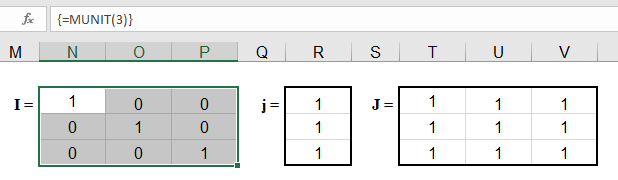
A simple way to create an n x n ones matrix (J) is to multiply the identity matrix by 0 and add 1, like this:
{ =1+0*MUNIT(n) }
The ones vector (j) of size n x 1 can be created by using INDEX to return the first column of the ones matrix, like this:
{ =INDEX(1+0*MUNIT(n),0,1) }
In older versions of Excel that don’t support the MUNIT function, you can create the ones vector, ones matrix and identity matrix using these formulas:
j =(1+0*ROW(INDIRECT("1:"&n)))
J =IF(ISERROR(OFFSET(INDIRECT("A1"),0,0,n,n)),1,1)
I =IF( ROW(OFFSET(INDIRECT("A1"),0,0,n,n)) = COLUMN(OFFSET(INDIRECT("A1"),0,0,n,n)), 1, 0)
Repeating Rows or Columns to Create a Matrix
Sometimes you may need to form a matrix by repeating a row or column. This can be done using MMULT and the ones vector.
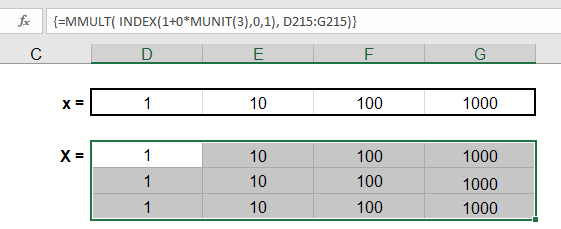
If you want to create a matrix with n rows by repeating row={1, 2, 3}, use the array formula =MMULT(j,row) where j is size n x 1.
{ =MMULT( INDEX(1+0*MUNIT(n),0,1), row) }
If you want to create a matrix with k columns by repeating col={1;2;3}, use the array formula =MMULT(col,TRANSPOSE(j)) where j is size k x 1.
{ =MMULT(col, TRANSPOSE(INDEX(1+0*MUNIT(k),0,1)) ) }
ROW or COLUMN Sums using the ONES Vector
It turns out that the ONES vector is very important in statistics for performing a very simple matrix operation: summing the rows or columns. Let’s say you have a range of size n (rows) x k (columns). You could either use the SUM function separately for each row or column, or you could use array formulas.
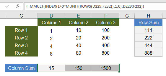
Column-Sum: To the sum the values within each COLUMN of the matrix and return the sums as a 1 x n array (or row vector), use
ones_vector =INDEX(1+0*MUNIT(ROWS(range)),0,1)
column_sum =MMULT(TRANSPOSE(ones_vector),range)
Row-Sum: To sum the values within each ROW of the matrix and return the sums as a k x 1 array (or column vector), use
ones_vector =INDEX(1+0*MUNIT(COLUMNS(range)),0,1)
row_sum =MMULT(range,ones_vector)
Creating a DIAGONAL Matrix
Element-wise multiplication of matrices can be used to create a Diagonal matrix. A Diagonal matrix is a special matrix where all of the off-diagonal terms are zeros. To create the Diagonal matrix, you multiply the matrix by the Identity matrix of the same size:
Diagonal =A*MUNIT(ROWS(A))
Many programs (but not Excel) include a function like diag(matrix) which returns an n x 1 vector containing the diagonal terms of an n x n matrix. To return the diagonal as a vector, you can use the row-sum operation on the Diagonal like this:
diag(A) =MMULT(A*MUNIT(ROWS(A)),(1+0*ROW(INDIRECT("1:"&ROWS(A)))))
Find the TRACE of a Square Matrix
The trace of a square matrix is just the sum of the diagonal elements. Therefore, the formula for calculating the trace is just:
trace(A) =SUM( A*MUNIT(ROWS(A)) )
Other Array Formula Examples
Linear Regression
The trend lines in an Excel chart allow you to do simple linear regression, but you can also do linear regression in Excel using matrix and array functions. It’s much easier to just use the LINEST function, but for fun I give the general formula for calculating the b matrix (the least squares estimators) when you have the y and X matrix. Or in other words, if you want to solve for b starting from y=Xb, you can do that using the formula b=(X‘X)-1X‘y which in Excel is:
{ =MMULT(MMULT(MINVERSE(MMULT(TRANSPOSE(x),x)),TRANSPOSE(x)),y) }
Alternate XNPV Function
If for some reason you don’t like Excel’s XNPV function or for some reason you need to use 360 days in a year instead of 365, you can use the following array formula in place of XNPV, where r is the discount rate.
{ =SUM(values_range/((1+r)^((date_range-INDEX(date_range,1))/365))) }
Running XIRR Formula
My Investment Tracker calculates an annualized compounded rate of return using a running XIRR array formula.
Some References for Array Formulas in Excel
- Guidelines and Examples of Array Formulas at support.office.com
- Array Formulas at cpearson.com — Some detailed information about using array formulas in Excel, along with some example array functions.
- Matrix Functions in Excel at bettersolutions.com — Examples showing the use of MDETERM, MINVERSE, MMULT, and TRANSPOSE.
- Using Excel to find Eigenvalues and Eigenvectors
- A.C.Rencher, Methods of Multivariate Analysis, John Wiley & Sons, Inc.: New York, 1995.
An array in Excel is a structure that holds a collection of values. Arrays can be mapped perfectly to ranges in a spreadsheet, which is why they are so important in Excel. An array can be thought of as a row of values, a column of values, or a combination of rows and columns with values. All cell references like A1:A5 and C1:F5 have underlying arrays, though the array structure is invisible in most contexts.
Example
In the example above, the three ranges map to arrays in a «row by column» scheme like this:
B5:D5 // 1 row x 3 columns
B8:B10 // 3 rows x 1 column
B13:D14  // 2 rows x 3 columns
If we display the values in these ranges as arrays, we have:
B5:D5={"red","green","blue"}
B8:B10={"red";"green";"blue"}
B13:D14={10,20,30;40,50,60}
Notice arrays must represent a rectangular structure.
Array syntax
All arrays in Excel are wrapped in curly brackets {} and the delimiters between array elements indicate rows and/or columns. In the US version of Excel, a comma (,) separates columns and a semicolon (;) separates rows. For example, both arrays below contain numbers 1-3, but one is horizontal and one is vertical:
{1,2,3} // columns (horizontal)
{1;2;3} // rows (vertical)
Text values in an array appear in double quotes («») like this:
{"a","b","c"}
To «see» the array associated with a range, start a formula with an equal sign (=) and select the range. Then use the F9 key to inspect the underlying array. You can also use the ARRAYTOTEXT function to show how columns and rows are represented. Set format to 1 (strict) to see the complete array.
Delimiters in other languages
In other language versions of Excel, the delimiters for rows and column can vary. For example, the Spanish version of Excel uses a backslash () for columns and a semicolon (;) for rows:
{123} // columns
{1;2;3} // rows
Arrays in formulas
Since arrays map directly to ranges, all formulas work with arrays in some way, though it isn’t always obvious. A simple example is a formula that uses the SUM function to sum the range A1:A5, which contains 10,15,20,25,30. Inside SUM, the range resolves to an array of values. SUM then sums all values in the array and returns a single result of 100:
=SUM(A1:A5)
=SUM({10;15;20;25;30})
=100
Note: you can use the F9 key to «see» arrays in your Excel formulas. See this video for a demo on using F9 to debug.
Array formulas
Array formulas involve an operation that delivers an array of results. For example, here is a simple array formula that returns the total count of characters in the range A1:A5:
=SUM(LEN(A1:A5))
Inside the LEN function, A1:A5 is expanded to an array of values. The LEN function then generates a character count for each value and returns an array of 5 results. The SUM function then returns the sum of all items in the array.
Dynamic arrays
With the introduction of Dynamic Array formulas in Excel, arrays have become more important, since it is easier than ever to write formulas that work with multiple results at the same time.