
Excel for Microsoft 365 Excel for Microsoft 365 for Mac Excel for the web Excel 2021 Excel 2021 for Mac Excel 2019 Excel 2019 for Mac Excel 2016 Excel 2016 for Mac Excel 2013 Excel 2010 Excel 2007 Excel for Mac 2011 Excel Starter 2010 More…Less
You use the SUMIF function to sum the values in a range that meet criteria that you specify. For example, suppose that in a column that contains numbers, you want to sum only the values that are larger than 5. You can use the following formula: =SUMIF(B2:B25,»>5″)

This video is part of a training course called Add numbers in Excel.
Tips:
-
If you want, you can apply the criteria to one range and sum the corresponding values in a different range. For example, the formula =SUMIF(B2:B5, «John», C2:C5) sums only the values in the range C2:C5, where the corresponding cells in the range B2:B5 equal «John.»
-
To sum cells based on multiple criteria, see SUMIFS function.
Important: The SUMIF function returns incorrect results when you use it to match strings longer than 255 characters or to the string #VALUE!.
Syntax
SUMIF(range, criteria, [sum_range])
The SUMIF function syntax has the following arguments:
-
range Required. The range of cells that you want evaluated by criteria. Cells in each range must be numbers or names, arrays, or references that contain numbers. Blank and text values are ignored. The selected range may contain dates in standard Excel format (examples below).
-
criteria Required. The criteria in the form of a number, expression, a cell reference, text, or a function that defines which cells will be added. Wildcard characters can be included — a question mark (?) to match any single character, an asterisk (*) to match any sequence of characters. If you want to find an actual question mark or asterisk, type a tilde (~) preceding the character.
For example, criteria can be expressed as 32, «>32», B5, «3?», «apple*», «*~?», or TODAY().
Important: Any text criteria or any criteria that includes logical or mathematical symbols must be enclosed in double quotation marks («). If the criteria is numeric, double quotation marks are not required.
-
sum_range Optional. The actual cells to add, if you want to add cells other than those specified in the range argument. If the sum_range argument is omitted, Excel adds the cells that are specified in the range argument (the same cells to which the criteria is applied).
Sum_range
should be the same size and shape as range. If it isn’t, performance may suffer, and the formula will sum a range of cells that starts with the first cell in sum_range but has the same dimensions as range. For example:
range
sum_range
Actual summed cells
A1:A5
B1:B5
B1:B5
A1:A5
B1:K5
B1:B5
Examples
Example 1
Copy the example data in the following table, and paste it in cell A1 of a new Excel worksheet. For formulas to show results, select them, press F2, and then press Enter. If you need to, you can adjust the column widths to see all the data.
|
Property Value |
Commission |
Data |
|---|---|---|
|
$100,000 |
$7,000 |
$250,000 |
|
$200,000 |
$14,000 |
|
|
$300,000 |
$21,000 |
|
|
$400,000 |
$28,000 |
|
|
Formula |
Description |
Result |
|
=SUMIF(A2:A5,»>160000″,B2:B5) |
Sum of the commissions for property values over $160,000. |
$63,000 |
|
=SUMIF(A2:A5,»>160000″) |
Sum of the property values over $160,000. |
$900,000 |
|
=SUMIF(A2:A5,300000,B2:B5) |
Sum of the commissions for property values equal to $300,000. |
$21,000 |
|
=SUMIF(A2:A5,»>» & C2,B2:B5) |
Sum of the commissions for property values greater than the value in C2. |
$49,000 |
Example 2
Copy the example data in the following table, and paste it in cell A1 of a new Excel worksheet. For formulas to show results, select them, press F2, and then press Enter. If you need to, you can adjust the column widths to see all the data.
|
Category |
Food |
Sales |
|---|---|---|
|
Vegetables |
Tomatoes |
$2,300 |
|
Vegetables |
Celery |
$5,500 |
|
Fruits |
Oranges |
$800 |
|
Butter |
$400 |
|
|
Vegetables |
Carrots |
$4,200 |
|
Fruits |
Apples |
$1,200 |
|
Formula |
Description |
Result |
|
=SUMIF(A2:A7,»Fruits»,C2:C7) |
Sum of the sales of all foods in the «Fruits» category. |
$2,000 |
|
=SUMIF(A2:A7,»Vegetables»,C2:C7) |
Sum of the sales of all foods in the «Vegetables» category. |
$12,000 |
|
=SUMIF(B2:B7,»*es»,C2:C7) |
Sum of the sales of all foods that end in «es» (Tomatoes, Oranges, and Apples). |
$4,300 |
|
=SUMIF(A2:A7,»»,C2:C7) |
Sum of the sales of all foods that do not have a category specified. |
$400 |
Top of Page
Need more help?

See also
SUMIFS function
COUNTIF function
Sum values based on multiple conditions
How to avoid broken formulas
VLOOKUP function
Need more help?
Adding up all the numbers in a single column or row in Excel is easy — the SUM function will work just fine. But what if you only want to sum cells that meet a certain condition – for example, to calculate the total sales generated by a specific product? In this case, Excel has a useful function called SUMIF to help you with the job!
Now, let’s go over what the SUMIF function is and how to use it with various examples, so you can see just how helpful this tool can be!
What is the SUMIF function in Excel?
The SUMIF function is a perfect choice when you’re looking for an easy way to aggregate certain data quickly. Unlike pivot tables, which may require more advanced knowledge in order to use correctly, SUMIF is relatively easy to get started with.
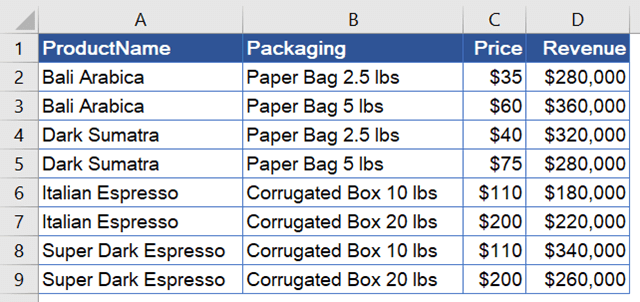
Here we have a spreadsheet that shows how much revenue was generated by each product and its packaging:
As you’re looking at the above data, the following questions might cross your mind:
- What is the total revenue generated by Bali Arabica?
- What is the total revenue generated from products with prices under $50?
- What is the total revenue generated from products packaged in paper bags?
The SUMIF function can help you answer those questions quickly. With it, you can sum values based on a single criteria, like those specified by the above questions.
Can I use SUMIF with multiple criteria?
SUMIF does not support multiple criteria. For example, you can’t use it to answer questions like: “What is the total revenue generated by products with paper bag packaging AND prices under $50?“. To work around this limitation, you’ll need to use the SUMIFS function, which is the more advanced version of SUMIF.
So, while SUMIF in Excel is powerful and easy to use, it does have its limitations. For that reason, you will find several examples in this article using SUMIFS as well as other functions as a workaround for solving cases that cannot be solved using SUMIF.
Excel SUMIF syntax and parameters
Syntax
=SUMIF(critera_range, criteria, [sum_range])Parameters or arguments
| Parameters | Description |
|---|---|
criteria_range |
Required. The range of cells that contains the criteria. |
criteria |
Required. The criteria used to determine which cells to add. It can be in the form of a number, expression, cell reference, text, or function.
Note: You need to use double quotation marks around any text criteria that include logical or mathematical symbols. If the criteria are numeric, you don’t need double quotes. You can also use logical operators as well as wildcards for partial matching, which makes the function powerful. Wildcards: – An asterisk ( – A tilde ( |
[sum_range] |
Optional. The range of cells to add. If you don’t specify this argument, Excel adds the cells that are specified in the criteria_range argument. |
How to use SUMIF in Excel: Basic usage
To have a good understanding of how to use the SUMIF function in Excel, let’s take a look at an example below. Suppose you want to find the total revenue generated by Bali Arabica, and want to store the result in G3.

To do that, follow the steps below:
Step 1: Position your cursor on G3 and start entering the formula.
=SUMIF(
Step 2: Enter the range of cells that contains the criteria, which is A2:A9.
=SUMIF(A2:A9
Step 3: Set your criteria in the second argument by typing "Bali Arabica".
=SUMIF(A2:A9,"Bali Arabica"
Note: You can type
"bali arabica"or"BALI ARABICA"because SUMIF is not case-sensitive. You can also add the “=” operator in the criteria ("=Bali Arabica"), but the equal sign (=) is not necessarily required when creating the “is equal to” criteria.
Step 4: Select a range of cells that you want to sum, which is D2:D9. After that, close the parentheses and press Enter.
=SUMIF(A2:A9,"Bali Arabica", D2:D9)

Let’s see what exactly happened:
- Excel searched for the word “Bali Arabica” in the range A2:A9
- If any row had that word, Excel added the revenue value in column D of the same row.
- In the end, you get the sum of all revenue for Bali Arabica.
Note: If your spreadsheet has many rows, using this formula that refers to the entire column may be more convenient:
=SUMIF(A:A,"Bali Arabica",D:D)
Now, if you’d like, try to calculate the revenue generated from Dark Sumatra, Italian Espresso, and Super Dark Espresso. You can follow the same steps as above (Step 1-4).
Alternatively, you can insert the SUMIF formula from the ribbon menu. To do that, click Formula, and then in the Function Library section, click Math & Trig. Look for the SUMIF function in the list and select it.

A popup will appear, allowing you to enter the function arguments. See the following arguments for Dark Sumatra. When done, click the OK button.

Excel SUMIF vs. SUMIFS
When talking about SUMIF, we really must also discuss SUMIFS. Both functions allow you to sum data based on certain conditions. The difference? SUMIF only supports a single criteria, whereas SUMIFS can handle multiple criteria.
SUMIFS syntax
=SUMIFS(sum_range, criteria_range1, criteria1, [criteria_range2, criteria2], …)The syntax is different from SUMIF in that you need to include the sum_range argument before any other arguments. Also, sum_range is a required argument, not optional like in the SUMIF function. Following the sum_range argument is the pair of the first criteria range and criteria (criteria_range1 and criteria1), and this pair of parameters is also required.
You can use SUMIFS even for one criteria (like SUMIF). You can add as many criteria as necessary, up to the limit of 127 pairs.
The basics of how to use these parameters are the same as SUMIF, so we won’t repeat the same explanation here. That means you won’t have to read a longer 😉
How to use SUMIF in Excel if your data is from different sources
Have you ever wanted to analyze data using Microsoft Excel, but your data is stored in external sources such as Jira, PipeDrive, Shopify, etc.? If yes, but you just couldn’t figure out how, our integration tool, Coupler.io, can help you. With this tool, you can import and combine data from different sources into Excel without coding. You can even automate the process on a schedule!
It’s important to note that your destination file needs to be an Excel Online file on OneDrive. If you want to use a file shared by another user, ensure you have edit access to the file.
To start using Coupler.io, sign up to it (it’s easy and no credit card is required). Then, all you need to do is create a new importer. A wizard will help you configure these three details:
- Source — You can take data from Airtable, Xero, Slack, Trello, and more.

- Destination — Select Microsoft Excel.

- Schedule— If you’d like, you can set up automatic data refresh on a schedule: hourly, daily, or monthly.

Pretty easy, right?! Once you finish setting up the importer and run it, your Excel file will be updated. Check out the available Excel integrations.
After that, you can start analyzing your data using Excel. 🙂
Common examples of how to use the SUMIF function in Excel
Understanding the basic use of SUMIF is one thing. But it’s better to be aware that there are many different ways to use this function. Now, let’s look at some common examples so we can get an idea of other fun things we can do with this function.
#1: Excel SUMIF if cells are equal to a value in another cell
With the data below, suppose you want to find out how many items were sold at $200. You can use this formula:
=SUMIF(B2:B9,200,C2:C9)
But instead of typing 200 manually as the second parameter, you can just refer to E3, as shown in the following formula:
=SUMIF(B2:B9,E3,C2:C9)

#2: If cells are not equal to
To calculate using the “not equal to” criteria, use the “<>” operator (with double quotes).
Now, assume that you want to calculate the total sales generated by products other than Rose in E3 and other than Daisy in E4. Use the following formulas:
- Not equal to Rose (E4):
=SUMIF(A2:A6,"<>Rose",B2:B6)
- Not equal to Daisy (E5):
=SUMIF(A2:A6,"<>"&D4,B2:B6)
Notice that for Daisy, we use a cell reference in the formula.

#3: If cells are less than / less than or equal to a number
Use the “<” operator to mean “less than” and “<=” to mean “less than or equal to“. The following example calculates the quantities of flowers with prices per stem that are:
- Less than $0.45 (F5):
=SUMIF(B2:B9,"<0.45",C2:C9)
- Less than or equal to $0.45 (F6):
=SUMIF(B2:B9,"<=0.45",C2:C9)

#4: If cell contains text
To sum if cells contain a specific text, you need to use a wildcard when specifying the criteria in the SUMIF function.
The following example calculates the total quantities of flowers with names containing “white“. Notice again that SUMIF is not case-sensitive. The formula in F5:
=SUMIF(A2:A9,"*white*",C2:C9)

#5: Excel SUMIF if cells contain an asterisk
Asterisks themselves are wildcards. So, to find text that contains an asterisk, you’ll need to use a tilde (~) to treat the character literally (not as a wildcard). The following example shows how to sum the amount for items that:
- Contain * (F5):
=SUMIF(B2:B9, "*~**", C2:C9)
- Contain * at the end (F6):
=SUMIF(B2:B9,"*~*",C2:C9)

#6: Excel SUMIF to sum values based on cells that are blank
Use double quotes without any space in between ("") in the criteria if you want to sum based on cells that are blank. Blank means empty or zero character length.
For the following spreadsheet, suppose you want to calculate the total bill for works that are still ongoing (not finished yet). To do that, you calculate the sum based on the finish dates that are blank using the following formula:
=SUMIF(C2:C11,"", D2:D11)

#7: Excel SUMIF to sum values based on cells that are not blank
Use the “not equal to” operator enclosed with double quotes (“<>“) in the criteria if you want to sum based on cells that are not blank.
Now, suppose you want to calculate the total bill only for works that are done (finish dates are not empty), use the following formula:
=SUMIF(C2:C11,"<>",D2:D11)

#8: If date is greater than, greater than or equal to
Use the “>” operator for greater than and “>=” for greater than or equal to. The following example sums the total bill for works that started:
- After Jun 5, 2021 (F5):
=SUMIF(B2:B11,">6/5/2021",C2:C11)
- On or after Jun 5, 2021 (F6):
=SUMIF(B2:B11,">="&DATE(2021,6,5),C2:C11)
Notice the formula in F6. You can also use the DATE function in the criteria.

Check out our guide dedicated to Excel SUMIF with Date Criteria.
#9: Excel SUMIF to sum values with the time format
Excel time values are actually numbers and you can sum them up using the SUMIF function like other numeric values. All you need to do is ensure that your data is in the correct time format. But how to set the correct time format? Well, it’s easy. Here’s an example:
Suppose you want to format Duration (column C) so that it uses the “h:mm:ss” format as shown in the following screenshot:

Follow the simple steps below:
Step 1: Select the entire column C (or only C2:C14 if you want to select this range only).
Step 2: Right-click and select Format Cells.
Step 3: Click Custom in the category list, then select h:mm:ss on the right.
Step 4: Click OK.
Now, let’s say you want to sum the total duration for Specialization 2. You can use the following formula:
=SUMIF(A2:A14,E4,C2:C14)

Note: When the sum of time can be greater than 24 hours, you should format the result cells to [h]:mm:ss to avoid the wrong total hours displayed in the results. That’s because for the normal time format like “h:mm:ss”, hours will reset to zero every 24 hours.
#10: With multiple OR criteria
To sum numbers based on other cells being equal to either one value or another, one of the solutions is by using multiple SUMIF functions in one formula.
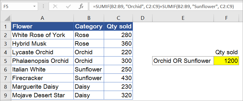
With the following table, suppose you want to sum the quantity sold for either Orchid OR Sunflower. To do that, you can use the following formula:
=SUMIF(B2:B9,"Orchid",C2:C9)+SUMIF(B2:B9,"Sunflower",C2:C9)
The solution here is very simple, and when there are only a few criteria, it often gets the job done quickly. However, if you want to sum values with more than three OR conditions (let’s say), then the formula will become long and complex. To avoid this problem, check out example #11 below, which uses a more advanced method that does not require adding up all of those different parts separately in order to get your total value.
Advanced examples of how to use the SUMIF function in Excel + without Excel SUMIF
Here are some more examples you may find helpful when summing values with criteria.
#11: Excel SUMIF with an array as the criteria argument
With the following data, suppose you want to sum the quantity sold for either Orchid OR Sunflower.

Notice that it uses multiple OR criteria, like in example #10. But this time, we’ll use an array in the criteria by following the steps below:
Step 1: List each condition separated by a comma and then enclose with curly brackets: {"Orchid","Sunflower"}
Step 2: Write the complete SUMIF formula using the array:
=SUMIF(B2:B9, {"Orchid","Sunflower"},C2:C9)
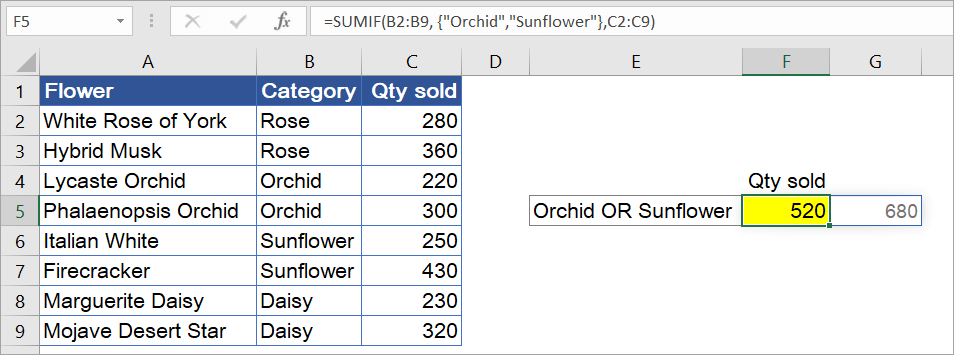
However, when you look at the result, the value is not correct. It only sums the total for Orchid, which is 520. And you’ll also see 680 next to it, which is the total for Sunflower. Why?
The SUMIF formula takes on an array argument that consists of two values. This forces the formula to return two results separately: 520 and 680. Since we put the formula in cell F5, the function only returns one result for this cell — i.e., the total for Orchid.
For this technique to work, you have to use one more step:
Step 3: Wrap your SUMIF formula in a SUM function, as follows:
=SUM(SUMIF(B2:B9, {"Orchid","Sunflower"},C2:C9))
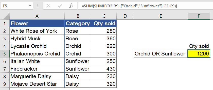
As you can see, the array criteria make the formula much more compact compared to multiple SUMIFs, as seen in example #10. You can also use arrays with numbers, but you don’t need to double-quote them.
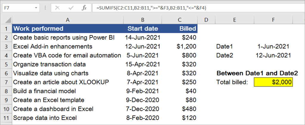
#12: With date range criteria (between two dates)
Unfortunately, the SUMIF Excel formula does not work for this case. Instead, you have to use SUMIFS.
With the following data, suppose you want to sum the total bill for works started between 1-Jun-2021 (cell F3) and 12-Jun-2021 (cell F4). Use the formula below:
=SUMIFS(C2:C11,B2:B11,">="&F3,B2:B11,"<="&F4)
#13: Excel SUMIF by month
Suppose you have the following table and want to find the total bill for works that started in June 2001. To get the result, you can use a SUMIFS function with these two criteria: start dates >= first day of June AND start dates <= last day of June.

Follow the steps below:
Step 1: Type the first date of June 2021 in E3.

Step 2: Change the format of E3 to “mmmm” to display the month name.

Step 3: Write the following formula to F3, then press Enter. Note: The EOMONTH function helps you to find the last day of the month.
=SUMIFS(C2:C11, B2:B11, ">="&E3,B2:B11,"<="&EOMONTH(E3,0))

#14: Excel SUMIF by year
Still using the same data with the previous example, suppose you want to find the total bill for works that started in 2020. To get the result, use SUMIFS with these two criteria: start dates >= first day of 2020 AND start dates <= last day of 2020.
=SUMIFS(C2:C11, B2:B11, ">="&DATE(E3,1,1),B2:B11,"<="&DATE(E3,12,31))

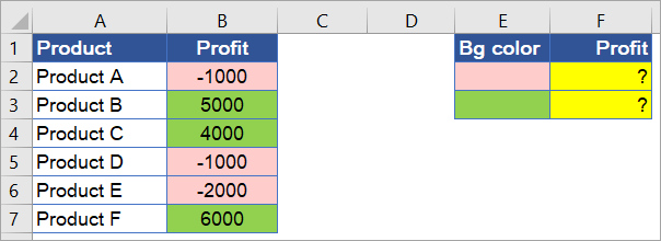
#15: Sum values based on background color
Suppose you have the following profit/loss data and want to sum based on the background color. In Excel, there is no default function to do that. But you can create an Excel VBA function to return the color index of a cell, and then use that index as the criteria in SUMIF.
Follow the steps below:
Step 1: Press Alt+F11 to open the Visual Basic Editor (VBE).
Step 2: Click Insert > Module.

Step 3: Copy-paste the following function to the editor:
Function ColorIndex(CellColor As Range)
    ColorIndex = CellColor.Interior.ColorIndex
End Function

Step 4: Type “Bg Color” as the header of column C. Then, type =ColorIndex(B2) in C2 and copy the formula down to C7.

Step 5: Use SUMIF to calculate the total profit based on the background color, as follows:
- Formula in F2:
=SUMIF(C2:C7, 19, B2:B7)
- Formula in F3:
=SUMIF(C2:C7, 43, B2:B7)

Read our guide on Excel SUMIFS VBA.
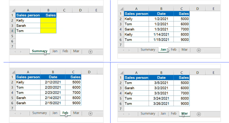
#16: Excel SUMIF to sum across multiple sheets
Suppose you have identical ranges in separate worksheets and want to summarize the total in the first worksheet, as shown in the following screenshot:
To do that, you can use the SUMIF function with INDIRECT, wrapped in SUMPRODUCT.
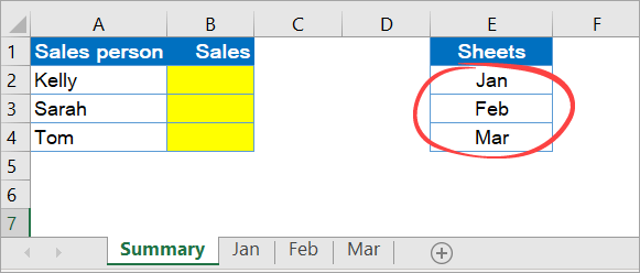
See the below steps to calculate the summary for the first salesperson (Kelly):
Step 1: List all the sheet names that are going to be summed in the Summary sheet. For example, in E2:E4 as shown below:
Step 2: Write a SUMIF formula for one sheet only – for example, Jan.
=SUMIF(Jan!A2:A6,Summary!A2,Jan!C2:C6)

Step 3: Nest the formula inside SUMPRODUCT.
=SUMPRODUCT(SUMIF(Jan!A2:A6,Summary!A2,Jan!C2:C6))
Step 4: Replace the sheet reference with a list of sheet names. In this case,
- Replace
Jan!A2:A6withINDIRECT("'"&E2:E4&"'!"&"A2:A6") - Replace
Jan!C2:C6withINDIRECT("'"&E2:E4&"'!"&"C2:C6")
The complete formula will be:
=SUMPRODUCT(SUMIF(INDIRECT("'"&E2:E4&"'!"&"A2:A6"),Summary!A2,INDIRECT("'"&E2:E4&"'!"&"C2:C6")))

#17: Sum multiple columns using one criteria
With the following data, suppose you want to calculate how many roses were sold in three months — Jan, Feb, and Mar. You can’t use either SUMIF or SUMIFS in this case. One alternative is to use the SUMPRODUCT function, as follows:
=SUMPRODUCT((A3:A11="Rose")*(B3:D11))

The first expression checks the range A3:A11 and returns an array of TRUE and FALSE. If any cell equals “Rose“, it will return TRUE, otherwise FALSE:
{TRUE;FALSE;FALSE;FALSE;FALSE;TRUE;TRUE;FALSE;FALSE}
The result above is then multiplied by the values in range B3:D11:
{500,400,300;400,500,200;500,300,400;300,400,500;400,200,500;400,500,200;600,200,300;400,300,200;400,500,300}
The SUMPRODUCT function will calculate the following values, which finally returns 3400.
=SUMPRODUCT({500,400,300;0,0,0;0,0,0;0,0,0;0,0,0;400,500,200;600,200,300;0,0,0;0,0,0})
Limitations of the Excel SUMIF function
After looking at these examples, we are sure you have your own conclusion about the limitations of the SUMIF function. But anyway, here’s the summary:
- You can’t use Excel SUMIF with multiple AND criteria. SUMIF is designed to handle one criteria only. As shown in example #10, you can use SUMIF + SUMIF for multiple OR conditions. However, you can’t use it with multiple AND criteria. For this case, use SUMIFS instead.
- You can’t use Excel SUMIF to sum multiple columns at once. As demonstrated in example #17, you can’t use either SUMIF and SUMIFS to sum multiple columns using one criteria. One of the solutions is to use the SUMPRODUCT function.
- You can’t use Excel SUMIF with an array as its range argument. In example #11, you can see that SUMIF accepts an array in its criteria argument. However, for its range argument, SUMIF requires a cell range. Because of this, you can’t use a formula that returns an array in its range argument — here’s an example:
Suppose you have the following table and want to sum the total bill for works that started in 2020; you can’t use this formula:
=SUMIF(TEXT(B2:B11,"yyyy"),"2020",C2:C11)

Why? That’s because the TEXT function in the above formula will return an array, which SUMIF doesn’t support.
What to do when your Excel SUMIF function is not working
There are times when you’ll find that your SUMIF formula in Excel is not working, or returns inaccurate results. There can be many reasons for that. Most of them have to do with incorrect ranges and defining criteria incorrectly. Thus, we recommend checking the following points:
- Check the order of the arguments used in the formula. For example, if you use three arguments, remember the first argument is the range that contains criteria, not the range you want to sum. You might have confused this with the SUMIFS formula.
- Check the range of cells you use, especially if you copy-pasted the formula from another cell. These include the range you want to sum as well as the range that contains the criteria.
- Ensure that you use double quotation marks (“”) for any criteria other than numeric.
- Check the format of the values involved in the calculation. For example, if you sum values with the time format, ensure you use the correct time format for your range values and the result cells.
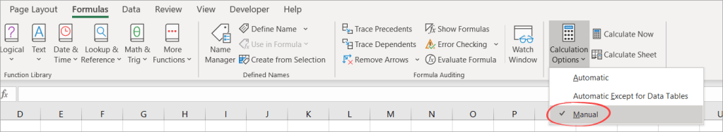
- You are sure that you’ve written the correct formula. Still, when you update the sheet, the SUMIF function doesn’t return the updated value? Well, in this case, check the formula calculation option in your spreadsheet. If it’s set to manual, press the F9 key to recalculate the sheet.
Finally, you’ve learned about the SUMIF function, including what it is, its syntax, how to use it, and its differences with SUMIFS. We also have covered various examples, as well as what to do when your function is not working.
We hope this article helped you, but if it didn’t, let us know if you have any comments or suggestions in the comments section below.
-

Senior analyst programmer

Back to Blog
Focus on your business
goals while we take care of your data!
Try Coupler.io
The SUMIF function sums cells in a range that meet a single condition, referred to as criteria. The SUMIF function is a common, widely used function in Excel, and can be used to sum cells based on dates, text values, and numbers. Note that SUMIF can only apply one condition. To sum cells using multiple criteria, see the SUMIFS function.
Syntax
The generic syntax for SUMIF looks like this:
=SUMIF(range,criteria,[sum_range])The SUMIF function takes three arguments. The first argument, range, is the range of cells to apply criteria to. The second argument, criteria, is the criteria to apply, along with any logical operators. The last argument, sum_range, is the range that should be summed. Note that sum_range is optional. If sum_range is not provided, SUMIF will sum cells in the first argument, range.
Examples: Basic Usage | Criteria in another cell | Not equal to | Blank cells | Dates | Wildcards | Videos
Applying criteria
The SUMIF function supports logical operators (>,<,<>,=) and wildcards (*,?) for partial matching. The tricky part about using the SUMIF function is the syntax needed to apply criteria. This is because SUMIF is in a group of eight functions that split logical criteria into two parts, range and criteria. Because of this design, operators need to be enclosed in double quotes («»). The table below shows examples of the syntax needed for common criteria:
| Target | Criteria |
|---|---|
| Cells greater than 75 | «>75» |
| Cells equal to 100 | 100 or «100» |
| Cells less than or equal to 100 | «<=100» |
| Cells equal to «Red» | «red» |
| Cells not equal to «Red» | «<>red» |
| Cells that are blank «» | «» |
| Cells that are not blank | «<>» |
| Cells that begin with «X» | «x*» |
| Cells less than A1 | «<«&A1 |
| Cells less than today | «<«&TODAY() |
Notice the last two examples involve concatenation with the ampersand (&) character. Any time you are using a value from another cell, or using the result of a formula in criteria with a logical operator like «<«, you will need to concatenate. This is because Excel needs to evaluate cell references and formulas to get a value before that value can be joined with an operator.
Limitations
There are a couple of limitations with SUMIF that you should be aware of. First, SUMIF only supports a single condition. If you need to sum cells using multiple criteria, use the SUMIFS function. Second, the SUMIF function requires an actual range for the range argument; you can’t substitute an array. This means you can’t do things like extract the year from a range that contains dates inside the SUMIF function. If you need to manipulate values that appear in the argument before applying criteria, the SUMPRODUCT function is a flexible solution.
Basic usage
With numbers in the range A1:A10, you can use SUMIF to sum cells greater than 5 like this:
=SUMIF(A1:A10,">5")If the range B1:B10 contains color names like «red», «blue», and «green», you can use SUMIF to sum numbers in A1:A10 when the color in B1:B10 is «red» like this:
=SUMIF(B1:B10,"red",A1:A10)Notice A1:A10 is now entered as the sum_range, because it is different from range, which contains only color names. To recap: criteria is applied to cells in range. When cells in range meet criteria, corresponding cells in sum_range are summed. The sum_range argument is optional. If sum_range is omitted, the cells in range are summed instead.
Worksheet example
In the worksheet shown, there are three SUMIF formulas. In the first formula (G5), SUMIF returns total Sales where Name = «jim». In the second formula (G6), SUMIF returns total Sales where State = «ca» (California). In the third formula (G7), SUMIF returns the total of Sales > 100:
=SUMIF(B5:B15,"jim",D5:D15) // name = "jim"
=SUMIF(C5:C15,"ca",D5:D15) // state = "ca"
=SUMIF(D5:D15,">100") // sales > 100
Notice the equals sign (=) is not required when constructing «is equal to» criteria. Also notice SUMIF is not case-sensitive; you can use «jim» or «Jim». Finally, notice that the last formula does not include sum_range, so range is summed instead.
Criteria in another cell
A value from another cell can be included in criteria using concatenation. In the example below, SUMIF will return the sum of all sales over the value in G4. Notice the greater than operator (>), which is text, must be enclosed in quotes. The formula in G5 is:
=SUMIF(D5:D9,">"&G4) // sum if greater than G4

Not equal to
To express «not equal to» criteria, use the «<>» operator surrounded by double quotes («»):

=SUMIF(B5:B9,"<>red",C5:C9) // not equal to "red"
=SUMIF(B5:B9,"<>blue",C5:C9) // not equal to "blue"
=SUMIF(B5:B9,"<>"&E7,C5:C9) // not equal to E7
Again notice SUMIF is not case-sensitive.
Blank cells
SUMIF can calculate sums based on cells that are blank or not blank. In the example below, SUMIF is used to sum the amounts in column C depending on whether column D contains «x» or is empty:

=SUMIF(D5:D9,"",C5:C9) // blank
=SUMIF(D5:D9,"<>",C5:C9) // not blank
Dates
The best way to use SUMIF with dates is to refer to a valid date in another cell, or use the DATE function. The example below shows both methods:

=SUMIF(B5:B9,"<"&DATE(2019,3,1),C5:C9)
=SUMIF(B5:B9,">="&DATE(2019,4,1),C5:C9)
=SUMIF(B5:B9,">"&E9,C5:C9)
Notice we must concatenate an operator to the date in E9. To use more advanced date criteria (i.e. all dates in a given month, or all dates between two dates) you’ll want to switch to the SUMIFS function, which can handle multiple criteria.
Wildcards
The SUMIF function supports wildcards, as seen in the example below:

=SUMIF(B5:B9,"mi*",C5:C9) // begins with "mi"
=SUMIF(B5:B9,"*ota",C5:C9) // ends with "ota"
=SUMIF(B5:B9,"????",C5:C9) // contains 4 characters
The tilde (~) is an escape character to allow you to find literal wildcards. For example, to match a literal question mark (?), asterisk(*), or tilde (~), add a tilde in front of the wildcard (i.e. ~?, ~*, ~~).
Average range caution
SUMIF makes certain assumptions about the size of sum_range, essentially resizing it when necessary to match the range argument, using the upper left cell in the range as an origin. In some cases, this behavior can create a result that seems reasonable but is in fact incorrect. For an example of this problem, see this article.
Notes
- SUMIF only supports one condition. Use the SUMIFS function for multiple criteria.
- When sum_range is omitted, the cells in range will be summed.
- Non-numeric criteria must be enclosed in double quotes (i.e. «<100», «>32», «TX»)
- Cell references in criteria are not enclosed in quotes, i.e. «<«&A1
- The wildcard characters ? and * can be used in criteria. A question mark matches any one character and an asterisk matches any sequence of characters (zero or more).
- To match a literal question mark(?) or asterisk (*), use a tilde (~) like (~?, ~*).
- SUMIF requires a range, you can’t substitute an array.

This Excel tutorial explains how to use the Excel SUMIF function with syntax and examples.
Description
The SUMIF function is a worksheet function that adds all numbers in a range of cells based on one criteria (for example, is equal to 2000).
The SUMIF function is a built-in function in Excel that is categorized as a Math/Trig Function. It can be used as a worksheet function (WS) in Excel. As a worksheet function, the SUMIF function can be entered as part of a formula in a cell of a worksheet.
To add numbers in a range based on multiple criteria, try the SUMIFS function.
![]() Subscribe
Subscribe
If you want to follow along with this tutorial, download the example spreadsheet.
Download Example
Syntax
The syntax for the SUMIF function in Microsoft Excel is:
SUMIF( range, criteria, [sum_range] )
Parameters or Arguments
- range
- The range of cells that you want to apply the criteria against.
- criteria
- The criteria used to determine which cells to add.
- sum_range
- Optional. It is the range of cells to sum together. If this parameter is omitted, it uses range as the sum_range.
Returns
The SUMIF function returns a numeric value.
Applies To
- Excel for Office 365, Excel 2019, Excel 2016, Excel 2013, Excel 2011 for Mac, Excel 2010, Excel 2007, Excel 2003, Excel XP, Excel 2000
Type of Function
- Worksheet function (WS)
Example (as Worksheet Function)
Let’s explore how to use SUMIF as a worksheet function in Microsoft Excel.
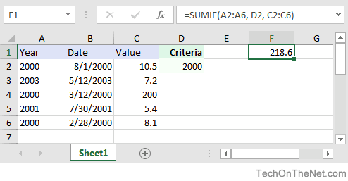
Based on the Excel spreadsheet above, the following SUMIF examples would return:
=SUMIF(A2:A6, D2, C2:C6)
Result: 218.6   'Criteria is the value in cell D2

=SUMIF(A:A, D2, C:C)
Result: 218.6   'Criteria applies to all of column A (ie: A:A)

=SUMIF(A2:A6, 2003, C2:C6)
Result: 7.2     'Criteria is the number 2003

=SUMIF(A2:A6, ">=2001", C2:C6)
Result: 12.6    'Criteria is greater than or equal to 2001

=SUMIF(C2:C6, "<100")
Result: 31.2    'Adds values in C2:C6 that are less than 100 (3rd parameter is omitted)
Now, let’s look at the example =SUMIF(A2:A6, D2, C2:C6) that returns a value of 218.6 and take a closer look why.
First Parameter
The first parameter in the SUMIF function is the range of cells that you want to apply the criteria against.
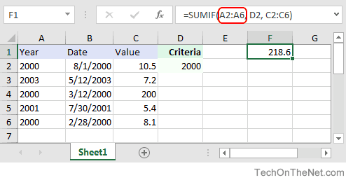
In this example, the first parameter is A2:A6. This is the range of cells that will be tested to determine if they meet the criteria.
Second Parameter
The second parameter in the SUMIF function is the criteria that will be applied against the range, A2:A6.
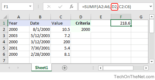
In this example, the second parameter is D2. This is a reference to the cell D2 which contains the numeric value, 2000. The SUMIF function will test each value in A2:A6 to see if it is equal to 2000.
Third Parameter
The third parameter in the SUMIF function is the range of numbers that will potentially be added together.
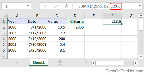
In this example, the third parameter is C2:C6. For every value in A2:A6 that matches D2, the corresponding value in C2:C6 will be summed.
Using Named Ranges
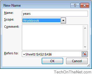
You can also use a named range in the SUMIF function. A named range is a descriptive name for a collection of cells or range in a worksheet. If you are unsure of how to setup a named range in your spreadsheet, read our tutorial on Adding a Named Range.
For example, if we created a named range called years in our spreadsheet that refers to cells A2:A6 in Sheet1 (Notice that the named range is an absolute reference that refers to =Sheet1!$A$2:$A$6 in the image below):
We could use this named range in our current example.
This would allow us to replace A2:A6 as the first parameter with the named range called years, as follows:
=SUMIF(A2:A6, D2, C2:C6)    'First parameter uses a standard range
Result: 218.6

=SUMIF(years, D2, C2:C6)    'First parameter uses a named range called years
Result: 218.6
Frequently Asked Questions
Question: I have a question about how to write the following formula in Excel.
I have a few cells, but I only need the sum of all the negative cells. So if I have 8 values, A1 to A8 and only A1, A4 and A6 are negative then I want B1 to be sum(A1,A4,A6).
Answer: You can use the SUMIF function to sum only the negative values as you described above. For example:
=SUMIF(A1:A8,"<0")
This formula would sum only the values in cells A1:A8 where the value is negative (ie: <0).
Question:In Microsoft Excel I’m trying to achieve the following with IF function:
If a value in any cell in column F is «food» then add the value of its corresponding cell in column G (eg a corresponding cell for F3 is G3). The IF function is performed in another cell altogether. I can do it for a single pair of cells but I don’t know how to do it for an entire column. Could you help?
At the moment, I’ve got this:
=IF(F3="food"; G3; 0)
Answer:This formula can be created using the SUMIF formula instead of using the IF function:
=SUMIF(F1:F10,"=food",G1:G10)
This will evaluate the first 10 rows of data in your spreadsheet. You may need to adjust the ranges accordingly.
I notice that you separate your parameters with semi-colons, so you might need to replace the commas in the formula above with semi-colons.
In this article, we will learn How to use the SUMIF function in Excel.
What is the SUMIF function ?
In Excel we calculate the sum having given criteria. For Example finding the sum of salaries which are greater than 50k or finding the sum of scores obtained by Jackie in Exams. This is usually a useful function when the given criteria is only one. Criteria range can be the same as sum range or can be different depending upon the situation.
SUMIF Function in Excel
=SUMIF(condition_range,condition,sum range)
Pro Notes:
- Conditions must be given using the double quotes («>15000»).
- If your sum range and condition range are the same, you can omit the sum_range variable in the SUMIF function. =SUMIF(E2:E10,»>15000″) and =SUMIF(E2:E10,»>15000″,E2:E10) will produce the same result, 56163.
- Text values are encapsulated in double quotes, but numbers do not. =SUMIF(C2:C10,103,E2:E10) this will work fine and will return 28026. However while working with logical operators you need to use double quotes. Like our example =SUMIF(D2:D10,»>70″,E2:E10)
- It can check only one condition. For multiple conditions we use the SUMIFS function in Excel.
Example :
All of these might be confusing to understand. Let’s understand how to use the function using an example. Here we will try out the SUMIF function. As the name suggests, the SUMIF formula in Excel sums values in a range on a given condition.
Generic Excel SUMIF Formula:
=SUMIF(condition_range,condition,sum range)
Let’s jump into an example. But theory…, Ah! We will cover it later.
Use SUMIF To Sum Values On One Condition
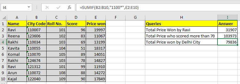
For this example I have prepared this data.
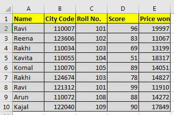
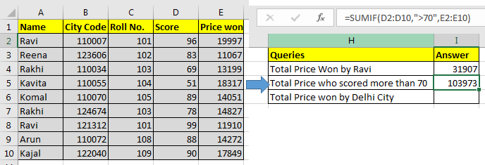
Based on this data we need to answer these questions:
Let’s start with the first question.
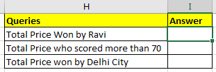
SUMIF with Text Condition
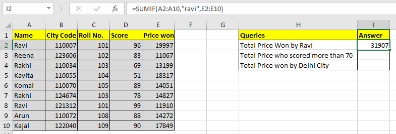
We need to tell the sum of the price won by Ravi.
So our condition range will be name range and that is A2:A10.
Our condition is Ravi and
Sum range is E2:E10.
So in cell I2 we will write:
=SUMIF(A2:A10,»ravi»,E2:E10)
Note that ravi is in double quotes. Text conditions are always written in double quotes. This is not the case with numbers.
Note that ravi is written in all smalls. Since SUMIF is not case sensitive, hence it doesn’t matter.
The above SUMIF formula will return 31907 as shown in the image below.
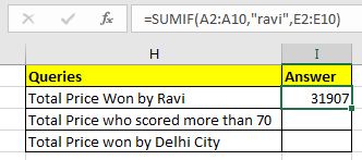
SUMIF with Logical Operators
For the second question, our condition range will be D2:D10.
Condition is >70 and
The sum range is the same as before.
=SUMIF(D2:D10,»>70″,E2:E10)
The above SUMIF formula will return 103973 as shown in the image below.
SUMIF with Wild Card Operators
In the third question, our condition is Delhi. But we don’t have a city column. Hmmm… So what do we have? Aha! City code. This will work.
We know that all Delhi city codes start from 1100. City codes are in 6 digits. So we know it is 1100??. “?” operator is used when we know number of characters but don’t know the character. As here we know that there are two more numbers after 1100. They can be anything, so we used “?”. If didn’t know the number of characters, we would use “*”.
Remember wild card operators only work with text values. Hence you need to convert city code into text.
You can concatenate numbers with “” to make them text value.
(formula to convert number into text) = number & “” or =CONCATENATE(number,””)
Now in cell I2 write this formula
=SUMIF(B2:B10,»1100??»,E2:E10)
This will return the sum of the price whose city code starts with 1100. In our example it is 79836.
Here are all the observational notes when error is given SUMIF function in Excel
Notes :
- If SUMIF is returning #N/A error or any other error, evaluate the formula. There is 80% chance that you will get your formula working. To evaluate formulas, select the formula cell and go to the Formula tab in ribbon. Here find Evaluate Formula option. You will find it in the Auditing section.
- If you are writing the correct formula and when you update the sheet, the SUMIF function doesn’t return an updated value. It is possible that you have set formula calculation to manual. Press F9 key to recalculate the sheet.
- Check the format of the values involved in the calculation. It is very likely to have unexpected formats if you have imported data from other sources.
Hope this article about How to use the SUMIF function in Excel is explanatory. Find more articles on calculating values and related Excel formulas here. If you liked our blogs, share it with your friends on Facebook. And also you can follow us on Twitter and Facebook. We would love to hear from you, do let us know how we can improve, complement or innovate our work and make it better for you. Write to us at info@exceltip.com.
Related Articles :
How to use the SUMPRODUCT function in Excel: Returns the SUM after multiplication of values in multiple arrays in excel.
SUM if date is between : Returns the SUM of values between given dates or period in excel.
Sum if date is greater than given date: Returns the SUM of values after the given date or period in excel.
2 Ways to Sum by Month in Excel: Returns the SUM of values within a given specific month in excel.
How to Sum Multiple Columns with Condition: Returns the SUM of values across multiple columns having condition in excel
How to use wildcards in excel : Count cells matching phrases using the wildcards in excel
Popular Articles :
How to use the IF Function in Excel : The IF statement in Excel checks the condition and returns a specific value if the condition is TRUE or returns another specific value if FALSE.
How to use the VLOOKUP Function in Excel : This is one of the most used and popular functions of excel that is used to lookup value from different ranges and sheets.
How to use the SUMIF Function in Excel : This is another dashboard essential function. This helps you sum up values on specific conditions.
How to use the COUNTIF Function in Excel : Count values with conditions using this amazing function. You don’t need to filter your data to count specific values. Countif function is essential to prepare your dashboard.