
SUM function
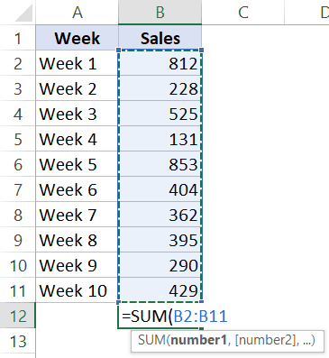
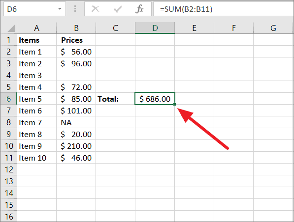
The SUM function adds values. You can add individual values, cell references or ranges or a mix of all three.
For example:
-
=SUM(A2:A10) Adds the values in cells A2:10.
-
=SUM(A2:A10, C2:C10) Adds the values in cells A2:10, as well as cells C2:C10.

SUM(number1,[number2],…)
|
Argument name |
Description |
|---|---|
|
number1 Required |
The first number you want to add. The number can be like 4, a cell reference like B6, or a cell range like B2:B8. |
|
number2-255 Optional |
This is the second number you want to add. You can specify up to 255 numbers in this way. |
This section will discuss some best practices for working with the SUM function. Much of this can be applied to working with other functions as well.
The =1+2 or =A+B Method – While you can enter =1+2+3 or =A1+B1+C2 and get fully accurate results, these methods are error prone for several reasons:
-
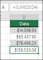
Typos – Imagine trying to enter more and/or much larger values like this:
-
=14598.93+65437.90+78496.23
Then try to validate that your entries are correct. It’s much easier to put these values in individual cells and use a SUM formula. In addition, you can format the values when they’re in cells, making them much more readable then when they’re in a formula.

-
-
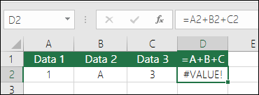
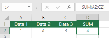
#VALUE! errors from referencing text instead of numbers
If you use a formula like:
-
=A1+B1+C1 or =A1+A2+A3
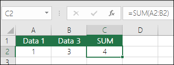
Your formula can break if there are any non-numeric (text) values in the referenced cells, which will return a #VALUE! error. SUM will ignore text values and give you the sum of just the numeric values.
-
-
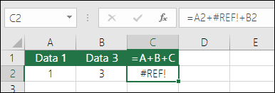
#REF! error from deleting rows or columns
If you delete a row or column, the formula will not update to exclude the deleted row and it will return a #REF! error, where a SUM function will automatically update.
-
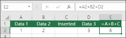
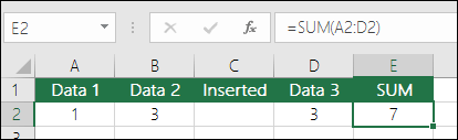
Formulas won’t update references when inserting rows or columns
If you insert a row or column, the formula will not update to include the added row, where a SUM function will automatically update (as long as you’re not outside of the range referenced in the formula). This is especially important if you expect your formula to update and it doesn’t, as it will leave you with incomplete results that you might not catch.
-
SUM with individual Cell References vs. Ranges
Using a formula like:
-
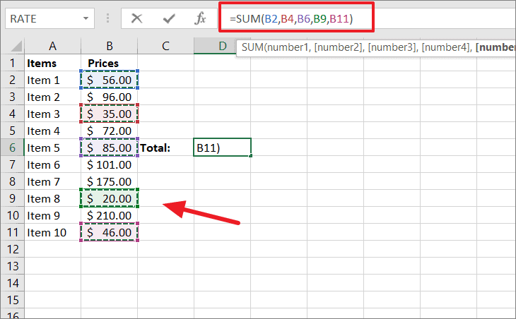
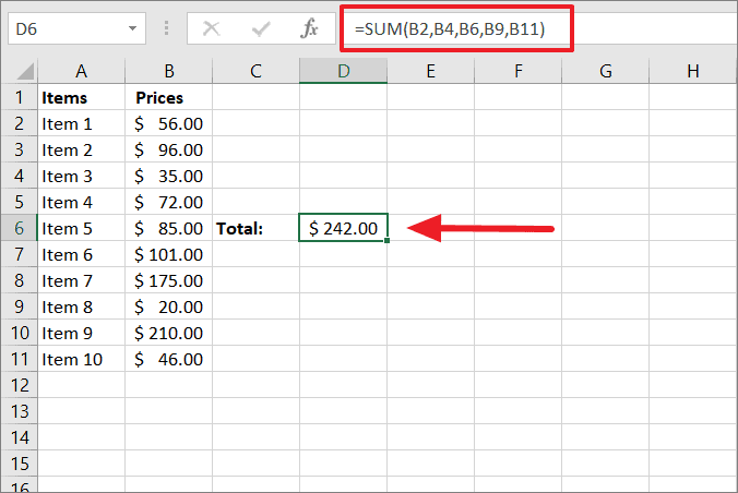
=SUM(A1,A2,A3,B1,B2,B3)
Is equally error prone when inserting or deleting rows within the referenced range for the same reasons. It’s much better to use individual ranges, like:
-
=SUM(A1:A3,B1:B3)
Which will update when adding or deleting rows.
-
-
I just want to Add/Subtract/Multiply/Divide numbers See this video series on Basic Math in Excel, or Use Excel as your calculator.
-
How do I show more/less decimal places? You can change your number format. Select the cell or range in question and use Ctrl+1 to bring up the Format Cells Dialog, then click the Number tab and select the format you want, making sure to indicate the number of decimal places you want.
-
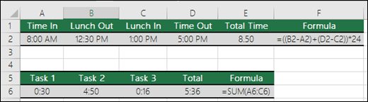
How do I add or subtract Times? You can add and subtract times in a few different ways. For example, to get the difference between 8:00 AM — 12:00 PM for payroll purposes you would use: =(«12:00 PM»-«8:00 AM»)*24, taking the end time minus the start time. Note that Excel calculates times as a fraction of a day, so you need to multiply by 24 to get the total hours. In the first example we’re using =((B2-A2)+(D2-C2))*24 to get the sum of hours from start to finish, less a lunch break (8.50 hours total).
If you’re simply adding hours and minutes and want to display that way, then you can sum and don’t need to multiply by 24, so in the second example we’re using =SUM(A6:C6) since we just need the total number of hours and minutes for assigned tasks (5:36, or 5 hours, 36 minutes).
For more information, see: Add or subtract time.
-
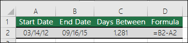
How do I get the difference between dates? As with times, you can add and subtract dates. Here’s a very common example of counting the number of days between two dates. It’s as simple as =B2-A2. The key to working with both Dates and Times is that you start with the End Date/Time and subtract the Start Date/Time.
For more ways to work with dates see: Calculate the difference between two dates.
-
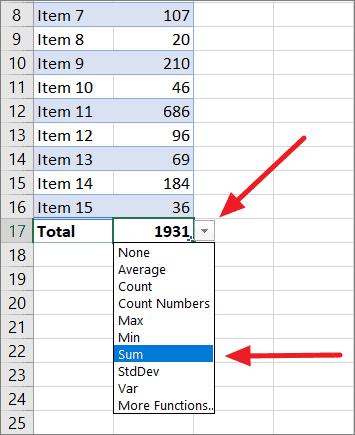
How do I sum just visible cells? Sometimes, when you manually hide rows or use AutoFilter to display only certain data you also only want to sum the visible cells. You can use the SUBTOTAL function. If you’re using a total row in an Excel table, any function you select from the Total drop-down will automatically be entered as a subtotal. See more about how to Total the data in an Excel table.
Need more help?
You can always ask an expert in the Excel Tech Community or get support in the Answers community.

See Also
Learn more about SUM
The SUMIF function adds only the values that meet a single criteria
The SUMIFS function adds only the values that meet multiple criteria
The COUNTIF function counts only the values that meet a single criteria
The COUNTIFS function counts only the values that meet multiple criteria
Overview of formulas in Excel
How to avoid broken formulas
Find and correct errors in formulas
Math & Trig functions
Excel functions (alphabetical)
Excel functions (by Category)
Need more help?
Содержание
- SUM function
- Need more help?
- Sum entire column
- Related functions
- Summary
- Generic formula
- Explanation
- Full column references
- Example
- Advantages and risks
- Alternatives
- How to Sum a Column in Excel (5 Really Easy Ways)
- Select and Get the SUM of the Column in Status Bar
- Get the SUM of a Column with AutoSum (with a Single-click/Shortcut)
- AutoSum Keyboard Shortcut
- Using the SUM Function to Manually calculate the Sum
- Sum Only the Visible Cells in a Column
- Convert Tabular Data to Excel Table to Get the Sum of Column
- Get the Sum of Column Based on a Criteria
SUM function
The SUM function adds values. You can add individual values, cell references or ranges or a mix of all three.
=SUM(A2:A10) Adds the values in cells A2:10.
=SUM(A2:A10, C2:C10) Adds the values in cells A2:10, as well as cells C2:C10.
The first number you want to add. The number can be like 4, a cell reference like B6, or a cell range like B2:B8.
This is the second number you want to add. You can specify up to 255 numbers in this way.
This section will discuss some best practices for working with the SUM function. Much of this can be applied to working with other functions as well.
The =1+2 or =A+B Method – While you can enter =1+2+3 or =A1+B1+C2 and get fully accurate results, these methods are error prone for several reasons:
Typos – Imagine trying to enter more and/or much larger values like this:
Then try to validate that your entries are correct. It’s much easier to put these values in individual cells and use a SUM formula. In addition, you can format the values when they’re in cells, making them much more readable then when they’re in a formula.
#VALUE! errors from referencing text instead of numbers
If you use a formula like:
Your formula can break if there are any non-numeric (text) values in the referenced cells, which will return a #VALUE! error. SUM will ignore text values and give you the sum of just the numeric values.
#REF! error from deleting rows or columns
If you delete a row or column, the formula will not update to exclude the deleted row and it will return a #REF! error, where a SUM function will automatically update.
Formulas won’t update references when inserting rows or columns
If you insert a row or column, the formula will not update to include the added row, where a SUM function will automatically update (as long as you’re not outside of the range referenced in the formula). This is especially important if you expect your formula to update and it doesn’t, as it will leave you with incomplete results that you might not catch.
SUM with individual Cell References vs. Ranges
Using a formula like:
Is equally error prone when inserting or deleting rows within the referenced range for the same reasons. It’s much better to use individual ranges, like:
Which will update when adding or deleting rows.
I just want to Add/Subtract/Multiply/Divide numbers See this video series on Basic Math in Excel, or Use Excel as your calculator.
How do I show more/less decimal places? You can change your number format. Select the cell or range in question and use Ctrl+1 to bring up the Format Cells Dialog, then click the Number tab and select the format you want, making sure to indicate the number of decimal places you want.
How do I add or subtract Times? You can add and subtract times in a few different ways. For example, to get the difference between 8:00 AM — 12:00 PM for payroll purposes you would use: =(«12:00 PM»-«8:00 AM»)*24, taking the end time minus the start time. Note that Excel calculates times as a fraction of a day, so you need to multiply by 24 to get the total hours. In the first example we’re using =((B2-A2)+(D2-C2))*24 to get the sum of hours from start to finish, less a lunch break (8.50 hours total).
If you’re simply adding hours and minutes and want to display that way, then you can sum and don’t need to multiply by 24, so in the second example we’re using =SUM(A6:C6) since we just need the total number of hours and minutes for assigned tasks (5:36, or 5 hours, 36 minutes).
For more information, see: Add or subtract time.
How do I get the difference between dates? As with times, you can add and subtract dates. Here’s a very common example of counting the number of days between two dates. It’s as simple as =B2-A2. The key to working with both Dates and Times is that you start with the End Date/Time and subtract the Start Date/Time.
How do I sum just visible cells? Sometimes, when you manually hide rows or use AutoFilter to display only certain data you also only want to sum the visible cells. You can use the SUBTOTAL function. If you’re using a total row in an Excel table, any function you select from the Total drop-down will automatically be entered as a subtotal. See more about how to Total the data in an Excel table.
Need more help?
You can always ask an expert in the Excel Tech Community or get support in the Answers community.
Источник
Sum entire column

Summary
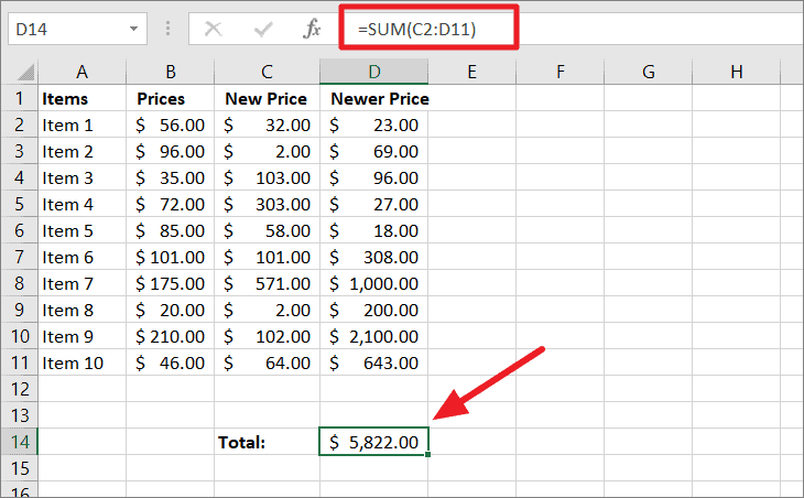
To sum an entire column without providing a specific range, you can use the SUM function with a full column reference. In the example shown, the formula in F5 is:
The result is the sum of all numbers in column D. As data is added to the table, the formula will continue to return a correct total.
Generic formula
Explanation
In this example, the goal is to return the total for an entire column in an Excel worksheet. One way to do this is to use a full column reference.
Full column references
Excel supports «full column» like this:
You can see how this works yourself by typing A:A or C:C into the name box (left of the formula bar) and hitting return. You will see Excel select the entire column.
Example
To solve the problem in the example worksheet, we can use a full column reference to column D with the SUM function like this:
The result is the sum of all numeric values in column D. One advantage to full column references is that they will automatically include new data. As entries are added to the table, the formula will automatically include the new amounts.
Advantages and risks
The main advantage to full column references is simplicity. Simple and very compact, a full column reference will automatically include all data in a column, even as data is added or removed. However, full column references come with certain risks. One risk is that you may accidentally include extra data in a calculation. For example, if you use =SUM(A:A) to sum numbers in column A, you are targeting over 1 million cells. If column A includes forgotten dates somewhere far below in the worksheet, the numeric value of these dates will be included, and SUM will return an incorrect result. Another risk is performance. Because so many cells are included, full column references can cause severe performance problems in certain worksheets or formulas.
Alternatives
There are good alternatives to full column references. If you need to target data that may change in size, a good solution is an Excel Table, which will automatically adapt to changing data. Another option is to use a dynamic named range.
Источник
How to Sum a Column in Excel (5 Really Easy Ways)
To get the sum of an entire column is something most of us have to do quite often. For example, if you have the sales data to date, you may want to quickly know the total sum in the column to the sales value till the present day.
You may want to quickly see what the total sum is or you may want is as a formula in a separate cell.
This Excel tutorial will cover a couple of quick and fast methods to sum a column in Excel.
This Tutorial Covers:
Select and Get the SUM of the Column in Status Bar
Excel has a status bar (at the bottom right of the Excel screen) which displays some useful statistics about the selected data, such as Average, Count, and SUM.
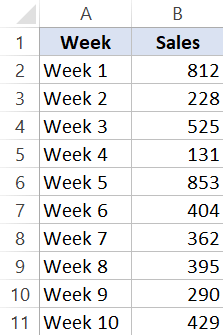
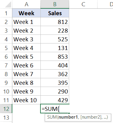
Suppose you have a dataset as shown below and you want to quickly know the sum of the sales for the given weeks.
To do this, select the entire Column B (you can do that by clicking on the B alphabet at the top of the column).
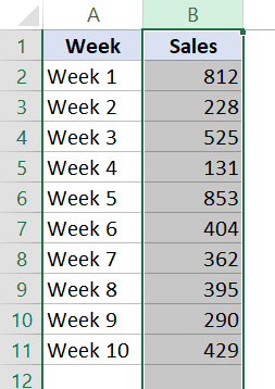
As soon as you select the entire column, you will notice that the status bar shows you the SUM of the column.

This is a really quick and easy way to get the sum of an entire column.
The good thing about using the status bar to get the sum of the column is that it ignores the cells that have the text and only considers the numbers. In our example, cell B1 has the text title, which is ignored and the sum of the column is displayed in the status bar.
In case you want to get the sum of multiple columns, you can make the selection, and it will show you the total sum value of all the selected columns.
In case you don’t want to select the entire column, you can make a range selection, and the status bar will show the sum of the selected cells only.
If you want, you can customize the status bar and get more data such as the maximum or the minimum value from the selection. To do this, right-click on the status bar and make the customizations.
Get the SUM of a Column with AutoSum (with a Single-click/Shortcut)
Autosum is a really awesome tool that allows you to quickly get the sum of an entire column with a single click.
Suppose you have the dataset as shown below and you want to get the sum of the values in column B.
Below are the steps to get the sum of the column:
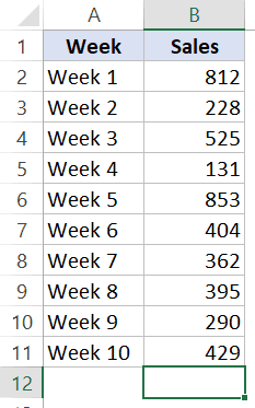
- Select the cell right below the last cell in the column for which you want the sum
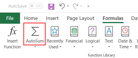
- Click the Formula tab
- In the Function Library group, click on the Autosum option
The above steps would instantly give you the sum of the entire column in the selected cell.
You can also use the Auto-sum by selecting the column that has the value and hitting the auto-sum option in the formula tab. As soon as you do this, it will give you the auto-sum in the cell below the selection.
Note: Autosum automatically detects the range and includes all the cells in the SUM formula. If you select the cell which has the sum and look at the formula in it, you will notice that it refers to all the cells above it in the column.
One minor irritant when using Autosum is that it would not identify the correct range in case there are any empty cells in the range or any cell has the text value. In the case of the empty cell (or text value), the auto-sum range would start below this cell.
AutoSum Keyboard Shortcut
While using the Autosum option in the Formula tab is fast enough, you can make getting the SUM even faster with a keyboard shortcut.
To use the shortcut, select the cell where you want the sum of the column and use the below shortcut:
Using the SUM Function to Manually calculate the Sum
While the auto-sum option is fast and effective, in some cases, you may want to calculate the sum of columns (or rows) manually.
One reason for doing this could be when you don’t want the sum of the entire column, but only of some of the cells in the column.
In such a case, you can use the SUM function and manually specify the range for which you want the sum.
Suppose you have a dataset as shown below and you want the sum of the values in column B:
Below are the steps to use the SUM function manually:
- Select the cell where you want to get the sum of the cells/range
- Enter the following: =SUM(
- Select the cells that you want to sum. You can use the mouse or can use the arrow key (with arrow keys, hold the shift key and then use the arrow keys to select range of cells).
- Hit the Enter key.
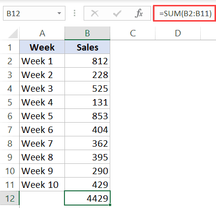
The above steps would give you the sum of the selected cells in the column.
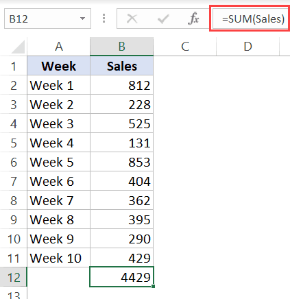
You can also create and use named ranges in the SUM function to quickly get the sum value. This could be useful when you have data spread on a large spreadsheet and you want to quickly get the sum of a column or range. You would first need to create a named range and then you can use that range name to get the sum.
Below is an example where I have named the range – Sales. The below formula also gives me the sum of the sales column:
Note that when you use the SUM function to get the sum of a column, it will also include the filtered or hidden cells.
In case you want the hidden cells to not be included when summing a column, you need to use the SUBTOTAL or AGGREGATE function (covered later in this tutorial).
Sum Only the Visible Cells in a Column
In case you have a dataset where you have filtered cells or hidden cells, you can not use the SUM function.
Below is an example of what can go wrong:
In the above example, when I sum the visible cells, it gives me the result as 2549, while the actual result of the sum of visible cells would be 2190.
The reason we get the wrong result is that the SUM function also takes the filtered/hidden cells when calculating the sum of a column.
In case you only want to get the sum of visible cells, you can’t use the SUM function. In this case, you need to use the AGGREGATE or SUBTOTAL function.
Below is the formula you can use to get the sum of only the visible cells in a column:
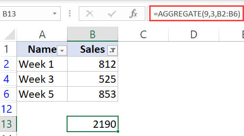
The Aggregate function takes the following arguments:
- function_num: This is a number that tells the AGGREGATE function the calculation that needs to be done. In this example, I have used 9 as I want the sum.
- options: In this argument, you can specify what you want to ignore when doing the calculation. In this example, I have used 3, which ‘Ignores hidden row, error values, nested SUBTOTAL, and AGGREGATE functions’. In short, it only uses the visible cells for the calculation.
- array: This is the range of cells for which you want to get the value. In our example, this is B2:B6 (which also has some hidden/filtered rows)
In case you’re using Excel 2007 or prior versions, you can use the following Excel formula:
Below is a formula where I show how to sum a column when there are filtered cells (using the SUBTOTAL function)
Convert Tabular Data to Excel Table to Get the Sum of Column
When you convert tabular data to an Excel Table, it becomes really easy to get the sum of columns.
I always recommend converting data into an Excel table, as it offers a lot of benefits. And with new tools such as Power Query, Power Pivot, and Power BI working so well with tables, it’s one more reason to use it.
To convert your data into an Excel table, follow the below steps:
- Select the data that you want to convert to an Excel Table
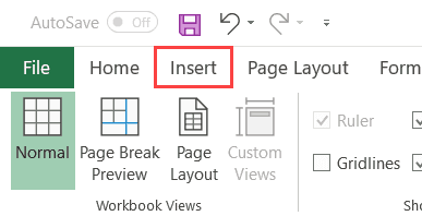
- Click the Insert tab
- Click on the Table icon
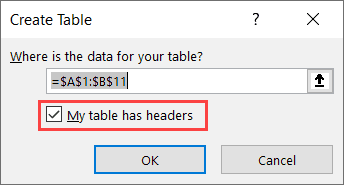
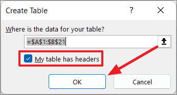
- In the Create Table dialog box, make sure the range is correct. Also, check the option ‘My table has headers’ in case you have headers in your data.
- Click Ok.
The above steps would convert your tabular data into an Excel Table.
Once you have the table in place, you can easily get the sum of all the columns.
Below are the steps to get the sum of the columns in an Excel Table:
- Select any cell in the Excel table
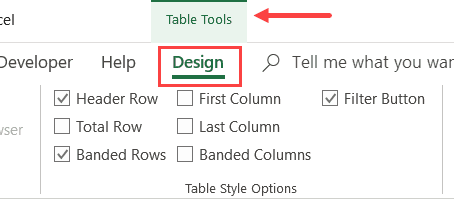
- Click the Design tab. This is a contextual tab that only appears when you select a cell in the Excel table.
- In the ‘Table Style Options’ group, check the ‘Total Row’ option
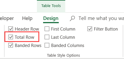
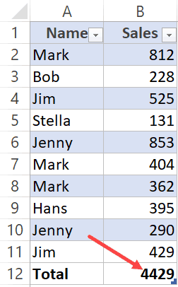
The above steps would instantly add a totals row at the bottom of the table and give the sum of all the columns.
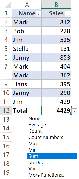
Another thing to know about using an Excel table is that you can easily change the value from the SUM of the column to Average, Count, Min/Max, etc.
To do this, select a cell in the totals rows and use the drop-down menu to select the value you want.
Get the Sum of Column Based on a Criteria
All the methods covered above would give you the sum of the entire column.
In case you want to only get the sum of those values that satisfy a criterion, you can easily do that with a SUMIF or SUMIFS formula.
For example, suppose you have the dataset as shown below and you only want to get the sum of those values that are more than 500.
You can easily do this using the below formula:
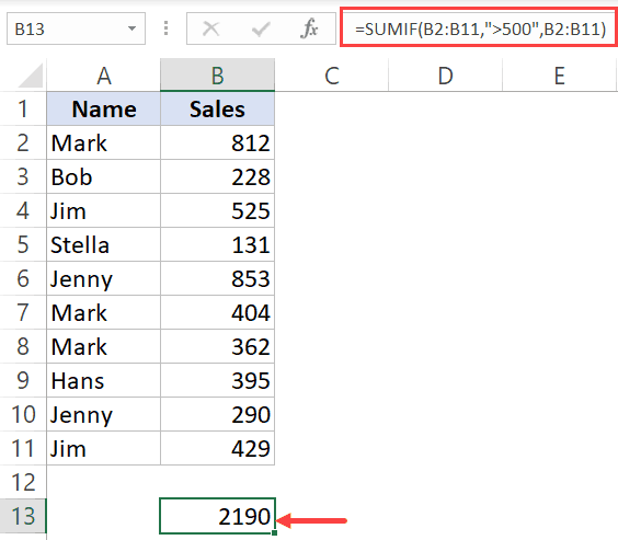
With the SUMIF formula, you can use a numeric condition as well as a text condition.
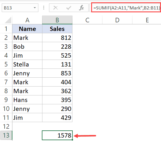
For example, suppose you have a dataset as shown below and you want to get the SUM of all the sales done by Mark.
In this case, you can use column A as the criteria range and “Mark” as the criteria, and the formula will give you the sum of all the values for Mark.
The below formula will give you the result:
You may also like the following Excel tutorials:
Источник
-
1
Определите какую колонку цифр или слов вы хотите сложить.
-
2
Выберите клетку для результата суммы.
-
3
Напишите знак равно и потом SUM. Вот так: =SUM
-
4
Напишите ссылку на первую клетку, потом двоеточие и ссылку на последнюю клетку. Вот так: =Sum(B4:B7).
-
5
Нажмите enter. Excel сложит номера в клетках B4 на B7
Реклама


-
1
Если у вас есть колонка с цифрами, используйте автосумму. Нажмите на клетку в конце списка, который вы хотите сложить (под цифрами).
- В Windows, нажмите Alt + = одновременно.
- На Mac, нажмите Command + Shift + T одновременно.
- Или на любом компьютере, вы можете нажать на кнопку Автосумма в меню/ленте Excel.
-
2
Убедитесь, что выделенные клетки – это те, которые вы хотите просуммировать.
-
3
Нажмите Enter для результата.
Реклама


-
1
Если у вас есть несколько колонок для сложения, наведите курсор на правую нижнюю часть клетки с результатом. Курсор изменит вид на крестик.
-
2
Удерживайте левую кнопки мышки и перетяните ее на клетки аналогичных колонок, сумму которых вы хотите получить.
-
3
Наведите мышку на последнюю клетку и отпустите. Excel автоматически заполнит результаты сумм выбранных колонок!
Реклама


Советы
- Как только вы начнете писать после знака =, Excel покажет выпадающий список доступных функций. Нажмите на функцию, которую хотите использовать, в нашем случае, на SUM.
- Представьте, что двоеточие – это слово НА, например, B4 НА B7.
Реклама
Об этой статье
Эту страницу просматривали 12 332 раза.
Была ли эта статья полезной?
Adding up columns or rows of numbers is something most of us are required to do quite often. For example, if you store crucial data such as sales records or price lists in the cells of a single column, you may want to quickly know the total of that column. So it’s necessary to know how to sum a column in Excel.
There are several ways you can sum or total a column/row in Excel including, using a single click, the AutoSum feature, SUM function, filter feature, SUMIF function, and by converting a dataset into a table. In this article, we will see the different methods for adding up a column or row in Excel.
SUM a Column with One Click using Status Bar
The easiest and quickest way to calculate the total value of a column is to click on the letter of the column with the numbers and check the ‘Status’ bar at the bottom. Excel has a Status bar at the bottom of the Excel window, which displays various information about an Excel worksheet including average, count, and sum value of the selected cells.
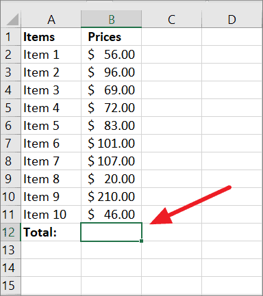
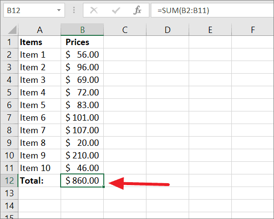
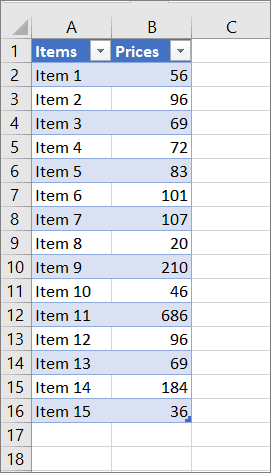
Let us assume you have a table of data as shown below and you want to find the total of the prices in column B.
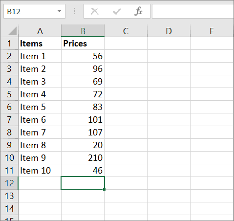
All you have to do is select the entire column with the numbers you want to sum (Column B) by clicking on the letter B at the top of the column and look at the Excel Status bar (next to the zoom control).
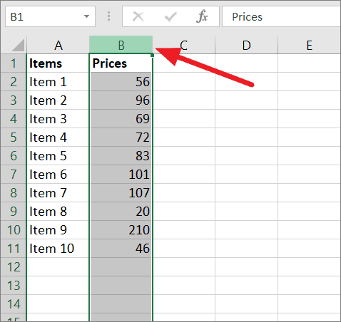
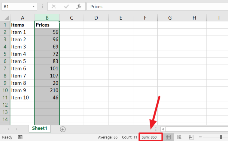
There you will see the total of the selected cells along with the average and count values.
You can also select data range B2 to B11 instead of the whole column and see the Status bar to know the total. You can also find the total of numbers in a row by selecting the row of values instead of a column.
The benefit of using this method is that it automatically ignores the cells with text values and only sums the numbers. As you can see above, when we selected the whole column B including cell B1 with a text title (Price), it only summed up the numbers in that column.
SUM a Column with AutoSum Function
Another quickest way to sum up a column in Excel is by using the AutoSum feature. AutoSum is a Microsoft Excel feature that allows you to quickly add up a range of cells (column or row) containing numbers/integers/decimals using the SUM function.
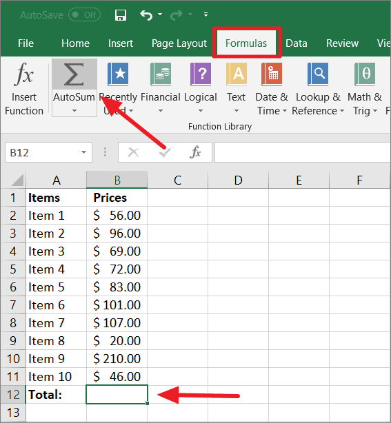
There is an ‘AutoSum’ command button on both the ‘Home’ and ‘Formula’ tab of the Excel ribbon that will insert the ‘SUM function’ in the selected cell when pressed.
Suppose you have the table of data as shown below and you want to sum up the numbers in column B. Select an empty cell right below the column or the right end of a row of data (to sum a row) you need to sum.
Then, select the ‘Formula’ tab and click on the ‘AutoSum’ button in the Function Library group.
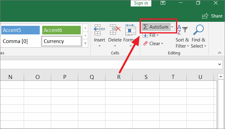
Or, go to the ‘Home’ tab and click on the ‘AutoSum’ button in the Editing group.
Either way, once you click the button, Excel will automatically insert the ‘=SUM()’ in the selected cell and highlights the range with your numbers (marching ants around the range). Check to see if the selected range is correct and if it’s not the correct range, you can change it by selecting another range. And the parameters of the function will auto-adjust according to that.
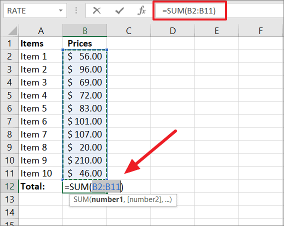
Then, just press Enter on your keyboard to see the sum of the entire column in the selected cell.
You can also invoke the AutoSum function using a keyboard shortcut.
To do that, select the cell, which is just below the last cell in the column for which you want the total, and use the below shortcut:
Alt+= (Press and hold the Alt key and press the equal sign = keyAnd it will automatically insert the SUM function and select the range for it. Then press Enter to total the column.
AutoSum lets you quickly sum a column or row with a single click or press of a keyboard shortcut.
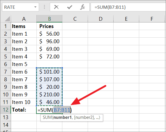
However, there is a certain limitation to the AutoSum function, it would not detect and select the correct range in case there are any empty cells in the range or any cell that has a text value.
As you can see in the above example, cell B6 is empty. And when we entered the AutoSum function in cell B12, it only selects 5 cells above. It’s because the function perceives that cell B7 is the end of the data and returns only 5 cells for the total.
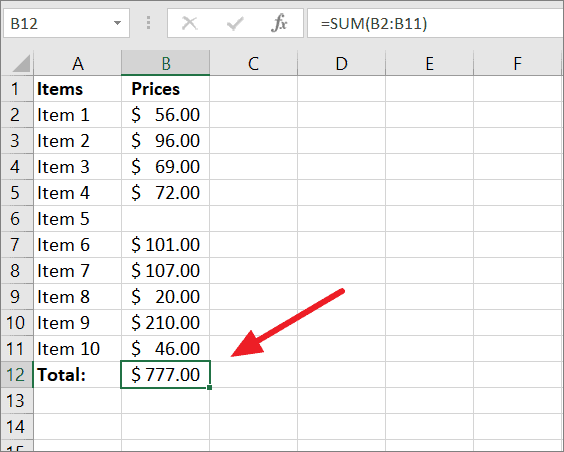
To fix this, you need to change the range by clicking-and-dragging with the mouse or type the correct cell references manually to highlight the whole column and press Enter. And, you will get the right result.
To avoid this, you can also enter the SUM function manually to calculate the sum.
SUM a Column by Entering the SUM Function Manually
Although the AutoSum command is quick and easy to use, sometimes, you may need to enter the SUM function manually to calculate the sum of a column or row in Excel. Especially, if you only want to add up some of the cells in your column or if your column contains any blanks cells or cells with a text value.
Also, if you want to show your sum value in any of the cells in the worksheet other than the cell right below the column or the cell after the row of numbers, you can use the SUM function. With the SUM function, you can calculate the sum or total of cells anywhere in the worksheet.
The Syntax of SUM Function:
=SUM(number1, [number2],...).number1(required) is the first numeric value to be added.number 2(optional) is the second additional numeric value to be added.
While number 1 is the required argument, you can sum up to a maximum of 255 additional arguments. The arguments can be the numbers you want to add up or cell references to the numbers.
Another benefit of using the SUM function manually is that you add up numbers in non-adjacent cells of a column or row as well as multiple columns or rows. Here’s how you use the SUM function manually:
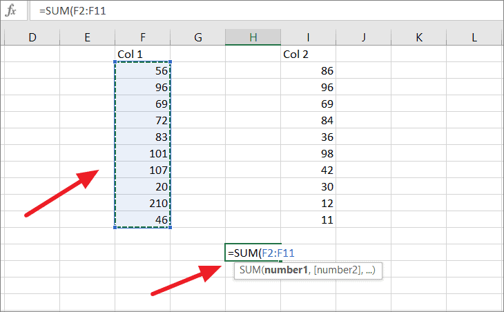
First, select the cell where you want to see the total of a column or row anywhere on the worksheet. Next, start your formula by typing =SUM( in the cell.
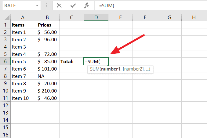
Then, select the range of cells with the numbers you want to sum or type the cell references for the range you want to sum in the formula.
You can either click-and-drag with the mouse or hold the shift key and then use the arrow keys to select a range of cells. If you want to enter cell reference manually, then type the cell reference of the first cell of the range, followed by a colon, followed by the cell reference of the last cell of the range.

After you entered the arguments, close the bracket and press the Enter key to get the result.
As you can see, even though the column has an empty cell and a text value, the function gives you the sum of all the selected cells.
Summing Non-Continous Cells in a Column
Instead of summing up a range of continuous cells, you can also sum up non-continuous cells in a column. To select non-adjacent cells, hold the Ctrl key and click the cells you want to add up or type cell references manually and separate them with comms (,) in the formula.
This will display the sum of only the selected cells in the column.
Summing Multiple Columns
If you want the sum of multiple columns, select multiple columns with the mouse or enter the cell reference of the first in the range, followed by a colon, followed by the last cell reference of the range for the arguments of the function.
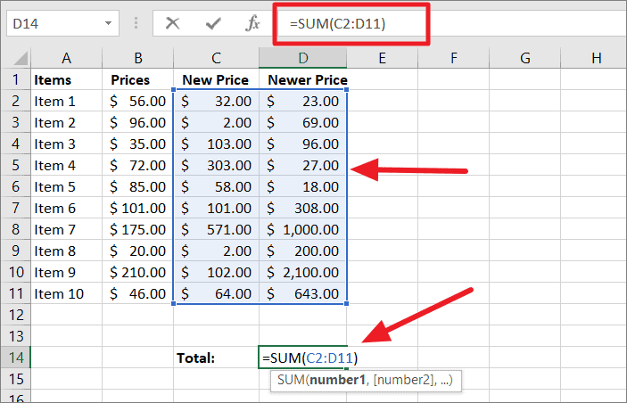
After you entered the arguments, close the bracket and press the Enter key to see the result.
Summing Non-Adjacent Columns
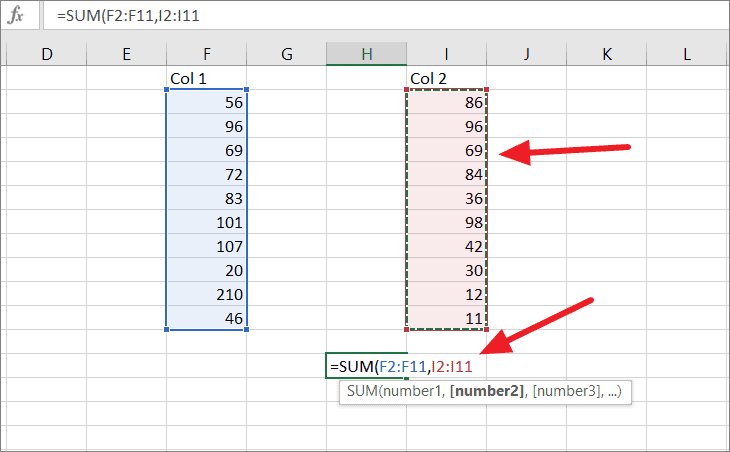
You can also sum non-adjacent columns using the SUM function. Here’s how:
Select any cell in the worksheet where you want to show the total of the non-adjacent columns. Then, start the formula by typing the function =SUM( in that cell. Next, select the first column range with the mouse or type the range reference manually.
Then, add a comma and select the next range or type the second range reference. You can add as many ranges as you want in this way and separate each of them with a comma (,).
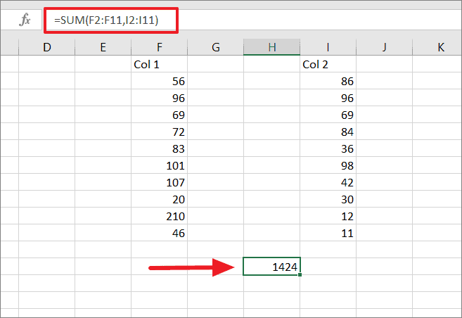
After the arguments, close the bracket, and press Enter to get the result.
Summing Column using Named Range
If you have a large worksheet of data and you want to quickly calculate the total of numbers in a column, you can use named ranges in the SUM function to find the total. When you create Named Ranges, you can use these names instead of the cell references which makes it easy to refer to data sets in Excel. It is easy to use named range in the function instead of scrolling down hundreds of rows to select the range.
Another good thing about using Named range is that you can refer to a data set (range) in another worksheet in the SUM argument and get the sum value in the current worksheet.
To use a named range in a formula, first, you need to create one. Here’s how you create and use a named range in the SUM function.
First, select the range of cells (without headers) for which you want to create a Named Range. Then, head to the ‘Formulas’ tab and click on the ‘Define Name’ button in the Defined Names group.
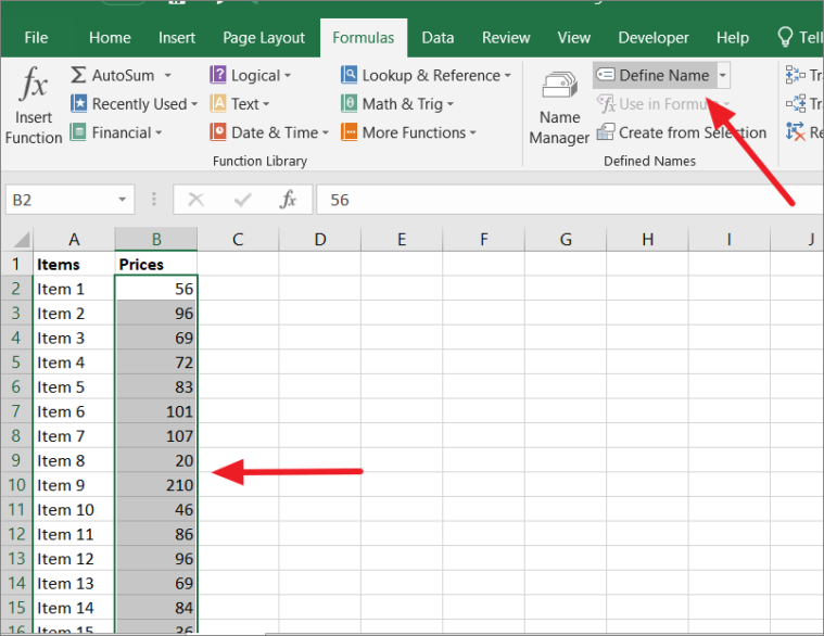
In the New Name dialogue box, specify the name you want to give to the selected range in the ‘Name:’ field. In the ‘Scope:’ field, you can change the scope of the named range as the whole Workbook or a specific worksheet. The scope specifies whether the named range would be available to the entire workbook or only a specific sheet. Then, click the ‘OK’ button.
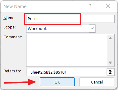
You can also change the reference of the range in the ‘Refers to’ field.
Alternatively, you can also name a range by using the ‘Name’ box. To do this, select the range, go to the ‘Name’ box on the left of the Formula bar (just above the letter A) and enter the name you wish to assign to the selected date range. Then, press Enter.
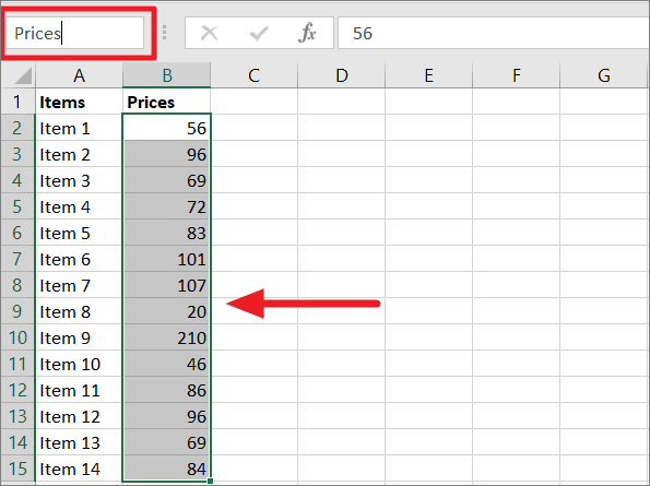
But when you create a named range using the Name box, it automatically sets the scope of the named range to the whole workbook.
Now, you can use the named range you created to quickly find the sum value.
To do this, select any empty cell anywhere on the workbook where you want to display the Sum result. And the type the SUM formula with the named range as is its arguments and press Enter:
=SUM(Prices)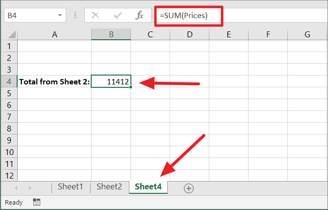
In the above example, the formula in Sheet 4 refers to the column named ‘Prices’ in Sheet 2 to get the sum of a column.
Sum Only the Visible Cells in a Column Using SUBTOTAL Function
If you have filtered cells or hidden cells in a data set or column, using the SUM function to total a column is not ideal. Because the SUM function includes filtered or hidden cells in its calculation.
The below example shows what happens when you sum a column with hidden or filtered rows:
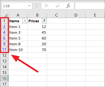
In the above table, we have filtered column B by prices that are less than 100. As a result, we have some filtered rows. You can notice that there are filtered/hidden rows in the table by the missing row numbers.
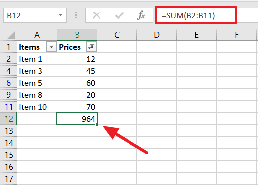
Now, when you sum the visible cells in column B using the SUM function, you should be getting ‘207’ as the sum value but instead, it shows ‘964’. Its because the SUM function also takes the filtered cells into account when calculating the sum.
This is why you cannot use the SUM function when filtered or hidden cells are involved.
If you don’t want the filtered/hidden cells to be included in the calculation when totaling a column and you only want to sum the visible cells, then you need to use the SUBTOTAL function.
SUBTOTAL Function
The SUBTOTAL is a powerful built-in function in Excel that allows you to perform various calculations (SUM, AVERAGE, COUNT, MIN, VARIANCE, and others) on a range of data and returns a total or an aggregate result of the column. This function only summarizes data in the visible cells while ignoring filtered or hidden rows. SUBTOTAL is a versatile function that can perform 11 different functions in visible cells of a column.
The Syntax of SUBTOTAL function:
=SUBTOTAL (function_num, ref1, [ref2], ...)Arguments:
function_num(required) – It is a function number that specifies which function to use for calculating the total. This argument can take any value from 1 to 11 or 101 to 111. Here, we need to sum the visible cells while ignoring filtered-out cells. For that, we need to use ‘9’.ref1(required) – The first named range or reference that you want to subtotal.ref2(optional) – The second named range or reference that you want to subtotal. After the first reference, you can add up to 254 additional references.
Summing a Column using SUBTOTAL Function
If you want to sum visible cells and exclude filtered or hidden cells, then follow these steps to use the SUBTOTAL function to sum a column:
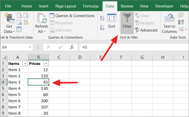
First, you need to filter your table. To do that, click on any cell within your data set. Then, navigate to the ‘Data’ tab and click the ‘Filter’ icon (funnel icon).
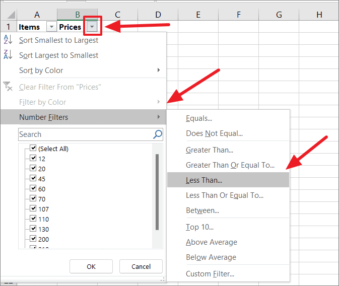
The arrows will appear next to column headers. Click on the arrow next to the column header with which you want to filter the table. Then, choose the filter option you wish to apply to your data. In the below example we want to filter column B with numbers less than 100.
In the Custom AutoFilter dialog box, we’re entering ‘100’ and clicking ‘OK’.
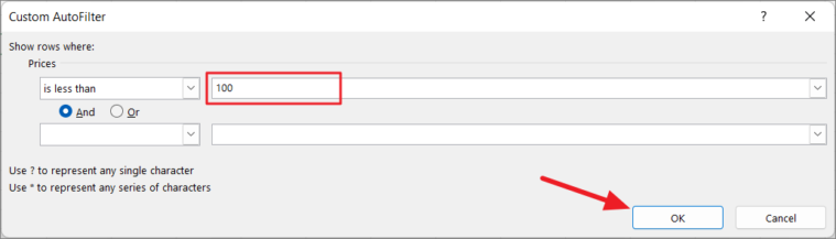
The numbers in the column are filtered by values less than 100.
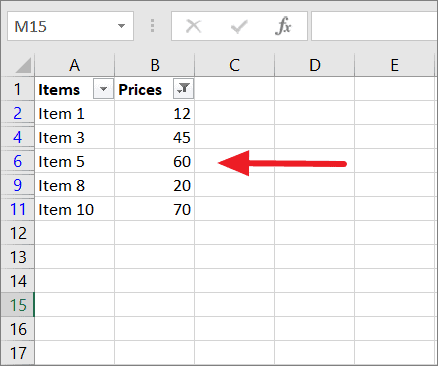
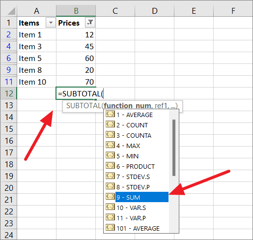
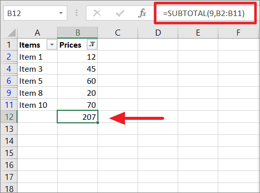
Now, select the cell where you wish to show the sum value and start typing the SUBTOTAL function. Once you open the SUBTOTAL function and type the bracket, you would see a list of functions you can use in the formula. Click ‘9 – SUM’ in the list or type ‘9’ manually as the first argument.
Then, select the range of cells you wish to sum or type the range reference manually and close the bracket. Then, press Enter.
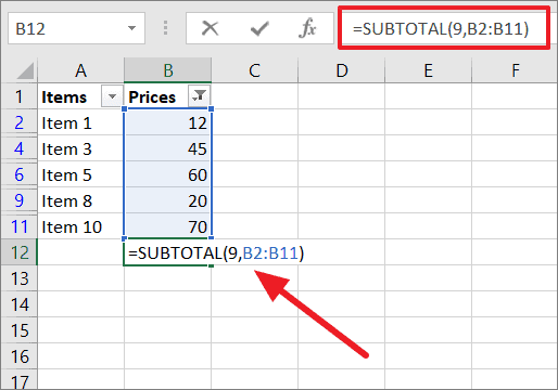
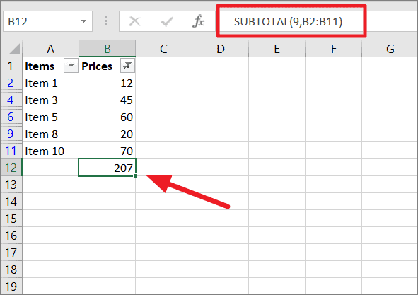
Now, you would get the sum (subtotal) of only the visible cells – ‘207’
Alternatively, you can also select the range (B2:B11) with the numbers that you wish to add up and click ‘AutoSum’ under the ‘Home’ or ‘Formulas’ tab.
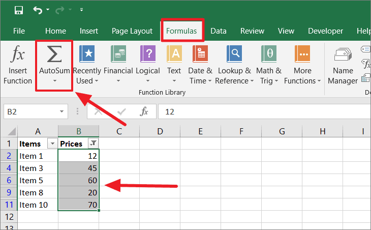
It will automatically add the SUBTOTAL function at the end of the table and sums up the result.
Convert Your Data into an Excel Table to Get the Sum of Column
Another easy way that you can use to sum your column is by converting your spreadsheet data into an Excel table. By converting your data into a table, you can not only sum your column but can also perform many other functions or operations with your list.
If your data is not already in a table format, you need to convert it into an Excel table. Here’s how you convert your data into an Excel table:
First, select any cell within the data set that you want to convert to an Excel Table. Then, go to the ‘Insert’ tab and click the ‘Table’ icon
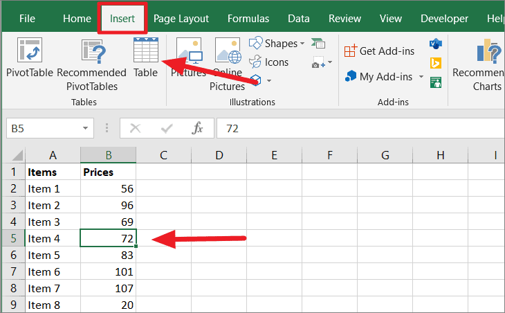
Or, you can press the shortcut Ctrl+T to convert the range of cells into an Excel Table.
In the Create Table dialog box, confirm the range and click ‘OK’. If your table has headers, leave the ‘My table has headers’ option checked.
This will convert your data set into an Excel Table.
Once, the table is ready, select any cell within the table. Then, navigate to the ‘Design’ tab which only appears when you select a cell in the table and check the box that says ‘Total Row’ under the ‘Table Style Options’ group.
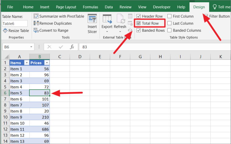
Once you have checked the ‘Total Row’ option, a new row would immediately appear at the end of your table with values at the end of each column (as shown below).
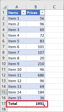
And when you click on a cell in that new row, you would see a drop-down next to that cell from which you can apply a function to get total. Select the cell at the last row (new row) of the column you want to sum, click the drop-down next to it, and make sure the ‘SUM’ function is selected from the list.
You can also change the function to Average, Count, Min, Max, and others to see their respective values in the new row.
Sum a Column Based on a Criteria
All the previous methods showed you how to calculate the total of the entire column. But what if you want to sum only specific cells that meet criteria rather than all of the cells. Then, you have to use the SUMIF function instead of the SUM function.
The SUMIF function looks for a specific condition in a range of cells (column) and then sums up the values that meet the given condition (or values corresponding to the cells that meet the condition). You can sum values based on number condition, text condition, date condition, wildcards as well as based on empty and non-empty cells.
Syntax of SUMIF Function:
=SUMIF(range, criteria, [sum_range])Arguments/Parameters:
range– The range of cells where we look for the cells that meet the criteria.criteria– The criteria that determine which cells need to be summed up. The criterion can be a number, text string, date, cell reference, expression, logical operator, wildcard character as well as other functions.sum_range(optional) – It is the data range with values to sum if the corresponding range entry matches the condition. If this argument is not specified, then the ‘range’ is summed instead.
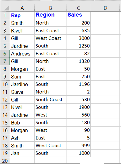
Suppose you have the below data set that contains sales data of each Rep from different regions and you only want to sum the sales amount from the ‘South’ region.
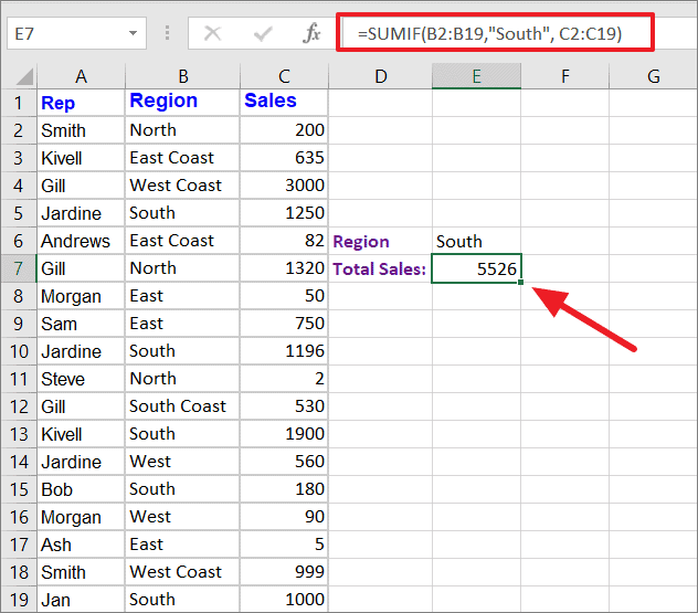
You can easily do that with the following formula:
=SUMIF(B2:B19,"South",C2:C19)Select the cell where you want to display the result and type this formula. The above SUMIF formula looks for the value ‘South’ in column B2:B19 and adds up the corresponding Sales amount in column C2:C19. Then displays the result in cell E7.
You can also refer to the cell that contains text condition instead of directly using the text in the criteria argument:
=SUMIF(B2:B19,E6,C2:C19)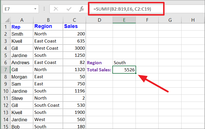
That’s it.