
Create, load, or edit a query in Excel (Power Query)
Excel for Microsoft 365 Excel 2021 Excel 2019 Excel 2016 Excel 2013 Excel 2010 More…Less
Power Query offers several ways to create and load Power queries into your workbook. You can also set default query load settings in the Query Options window.
Tip To tell if data in a worksheet is shaped by Power Query, select a cell of data, and if the Query context ribbon tab appears, then the data was loaded from Power Query.
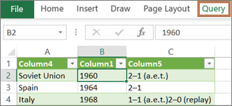
Know which environment you’re in Power Query is well-integrated into the Excel user interface, especially when you import data, work with connections, and edit Pivot Tables, Excel tables, and named ranges. To avoid confusion, it’s important to know which environment you are currently in, Excel or Power Query, at any point in time.
|
The familiar Excel worksheet , ribbon, and grid |
The Power Query Editor ribbon and data preview |
|
|
For example, manipulating data in an Excel worksheet is fundamentally different than Power Query. Furthermore, the connected data that you see in an Excel worksheet, may or may not have Power Query working behind the scenes to shape the data. This only occurs when you load the data to a worksheet or Data Model from Power Query.
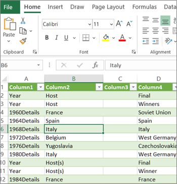
Rename worksheet tabs It’s a good idea to rename worksheet tabs in a meaningful way, especially if you have a lot of them. It’s particularly important to clarify the difference between a worksheet of data, and a worksheet loaded from the Power Query Editor. Even if you have only two worksheets, one with an Excel table, called Sheet1, and the other a query created by importing that Excel table, called Table1, it’s easy to get confused. It’s always good practice to change the default names of worksheet tabs to names that make more sense to you. For example, rename Sheet1 to DataTable and Table1 to QueryTable. Now it’s clear which tab has the data and which tab has the query.
You can either create a query from imported data or create a blank query.
Create a query from imported data
This is the most common way to create a query.
-
Import some data. For more information, see Import data from external data sources.
-
Select a cell in the data and then select Query > Edit.
Create a blank query
You may want to just start from scratch. There are two ways to do this.
-
Select Data > Get Data > From Other Sources > Blank Query.
-
Select Data > Get Data > Launch Power Query Editor.
At this point, you can manually add steps and formulas if you know the Power Query M formula language well.
Or you can select Home and then select a command in the New Query group. Do one of the following.
-
Select New Source to add a data source. This command is just like the Data > Get Data command in the Excel ribbon.
-
Select Recent Sources to select from a data source you have been working with. This command is just like the Data > Recent Sources command in the Excel ribbon.
-
Select Enter Data to manually enter data. You might choose this command to try out the Power Query Editor independent of an external data source.
Assuming your query is valid and has no errors, you can load it back to a worksheet or Data Model.
Load a query from the Power Query Editor
In the Power Query Editor, do one of the following:
-
To load to a worksheet, select Home > Close & Load > Close & Load.
-
To load to a Data Model, select Home > Close & Load > Close & Load To.
In the Import Data dialog box, select Add this data to the Data Model.
Tip Sometimes the Load To command is dimmed or disabled. This can occur the first time you create a query in a workbook. If this occurs, select Close & Load, in the new worksheet, select Data > Queries & Connections > Queries tab, right click the query, and then select Load To. Alternatively, on the Power Query Editor ribbon select Query > Load To.
Load a query from the Queries and Connections pane
In Excel, you may want to load a query into another worksheet or Data Model.
-
In Excel, select Data > Queries & Connections, and then select the Queries tab.
-
In the list of queries, locate the query, right click the query, and then select Load To. The Import Data dialog box appears.
-
Decide how you want to import the data, and then select OK. For more information about using this dialog box, select the question mark (?).
There are several ways to edit a query loaded to a worksheet.
Edit a query from data in Excel worksheet
-
To edit a query, locate one previously loaded from the Power Query Editor, select a cell in the data, and then select Query > Edit.
Edit a query from the Queries & Connections pane
You may find the Queries & Connections pane is more convenient to use when you have many queries in one workbook and you want to quickly find one.
-
In Excel, select Data > Queries & Connections, and then select the Queries tab.
-
In the list of queries, locate the query, right click the query, and then select Edit.
Edit a query from the Query Properties dialog box
-
In Excel, select Data > Data & Connections > Queries tab, right click the query and select Properties, select the Definition tab in the Properties dialog box, and then select Edit Query.
Tip If you are in a worksheet with a query, select Data > Properties, select the Definition tab in the Properties dialog box, and then select Edit Query.
A Data Model typically contains several tables arranged in a relationship. You load a query to a Data Model by using the Load To command to display the Import Data dialog box, and then selecting the Add this data to the Data Model check box. For more information about Data Models, see Find out which data sources are used in a workbook data model, Create a Data Model in Excel, and Use multiple tables to create a PivotTable.
-
To open the Data Model, select Power Pivot > Manage.
-
At the bottom of the Power Pivot window, select the worksheet tab of the table you want.
Confirm that the correct table displays. A Data Model can have many tables.
-
Note the name of the table.
-
To close the Power Pivot window, select File > Close. It may take a few seconds to reclaim memory.
-
Select Data > Connections & Properties > Queries tab, right click the query, and then select Edit.
-
When finished making changes in the Power Query Editor, select File > Close & Load.
Result
The query in the worksheet and the table in the Data Model are updated.
If you notice that loading a query to a Data Model takes much longer than loading to a worksheet, check your Power Query steps to see if you are filtering a text column or a List structured column by using a Contains operator. This action causes Excel to enumerate again through the entire data set for each row. Furthermore, Excel can’t effectively use multithreaded execution. As a workaround, try using a different operator such as Equals or Begins With.
Microsoft is aware of this problem and it is under investigation.
You can load a Power Query:
-
To a worksheet. In the Power Query Editor, select Home > Close & Load > Close & Load.
-
To a Data Model. In the Power Query Editor, select Home > Close & Load > Close & Load To.
By default, Power Query loads queries to a new worksheet when loading a single query, and loads multiple queries at the same time to the Data Model. You can change the default behavior for all your workbooks or just the current workbook. When setting these options, Power Query doesn’t change query results in the worksheet or the Data Model data and annotations.
You can also dynamically override the default settings for a query by using the Import dialog box which displays after you select Close & Load To.
Global settings that apply to all your workbooks
-
In the Power Query Editor, select File > Options and settings > Query Options.
-
In the Query Options dialog box, on the left side, under the GLOBAL section, select Data Load.
-
Under the Default Query Load Settings section, do the following:
-
Select Use standard load settings.
-
Select Specify custom default load settings, and then select or clear Load to worksheet or Load to Data Model.
-
Tip At the bottom of the dialog box, you can select Restore Defaults to conveniently return to the default settings.
Workbook settings that only apply to the current workbook
-
In the Query Options dialog box, on the left side, under the CURRENT WORKBOOK section, select Data Load.
-
Do one or more of the following:
-
Under Type Detection, select or clear Detect column types and headers for unstructured sources.
The default behavior is to detect them. Clear this option if you prefer to shape the data yourself.
-
Under Relationships, select or clear Create relationships between tables when adding to the Data Model for the first time.
Before loading to the Data Model, the default behavior is to find existing relationships between tables, such as foreign keys in a relational database and import them with the data. Clear this option if you prefer to do this on your own.
-
Under Relationships, select or clear Update relationships when refreshing queries loaded to the Data Model.
The default behavior is to not update relationships. When refreshing queries already loaded to the Data Model, Power Query finds existing relationships between tables such as foreign keys in a relational database and updates them. This might remove relationships created manually after the data was imported or introduce new relationships. However, if you want to do this, select the option.
-
Under Background Data, select or clear Allow data previews to download in the background.
The default behavior is to download data previews in the background. Clear this option if you can want to see all the data right away.
-
See Also
Power Query for Excel Help
Manage queries in Excel
Need more help?
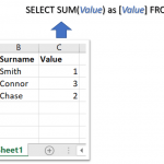
You can use Microsoft Query in Excel to retrieve data from an Excel Workbook as well as External Data Sources using SQL SELECT Statements. Excel Queries created this way can be refreshed and rerun making them a comfortable and efficient tool in Excel.
Microsoft Query allows you use SQL directly in Microsoft Excel, treating Sheets as tables against which you can run Select statements with JOINs, UNIONs and more. Often Microsoft Query statements will be more efficient than Excel formulas or a VBA Macro. A Microsoft Query (aka MS Query, aka Excel Query) is in fact an SQL SELECT Statement. Excel as well as Access use Windows ACE.OLEDB or JET.OLEDB providers to run queries. Its an incredible often untapped tool underestimated by many users!
What can I do with MS Query?
 Using MS Query in Excel you can extract data from various sources such as:
- Excel Files – you can extract data from External Excel files as well as run a SELECT query on your current Workbook
- Access – you can extract data from Access Database files
- MS SQL Server – you can extract data from Microsoft SQL Server Tables
- CSV and Text – you can upload CSV or tabular Text files
Step by Step – Microsoft Query in Excel
In this step by step tutorial I will show you how to create an Microsoft Query to extract data from either you current Workbook or an external Excel file.
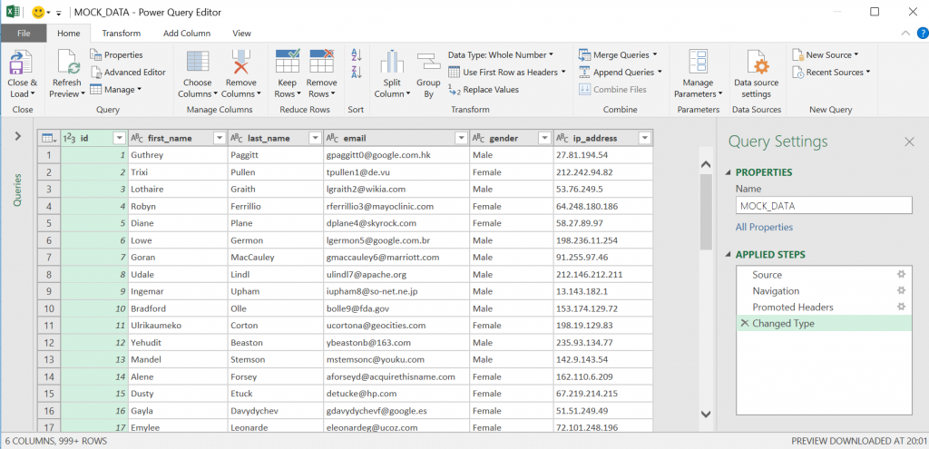
I will extract data from an External Excel file called MOCK DATA.xlsx. In this file I have a list of Male/Female mock-up customers. I will want to create a simple query to calculate how many are Male and how many Female.
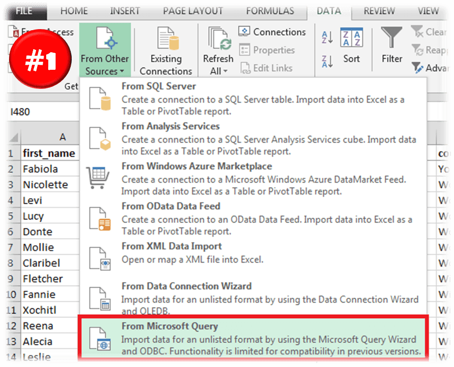
Open the MS Query (from Other Sources) wizard
Go to the DATA Ribbon Tab and click From Other Sources. Select the last option From Microsoft Query.
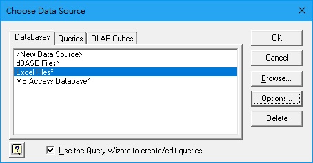
Select the Data Source
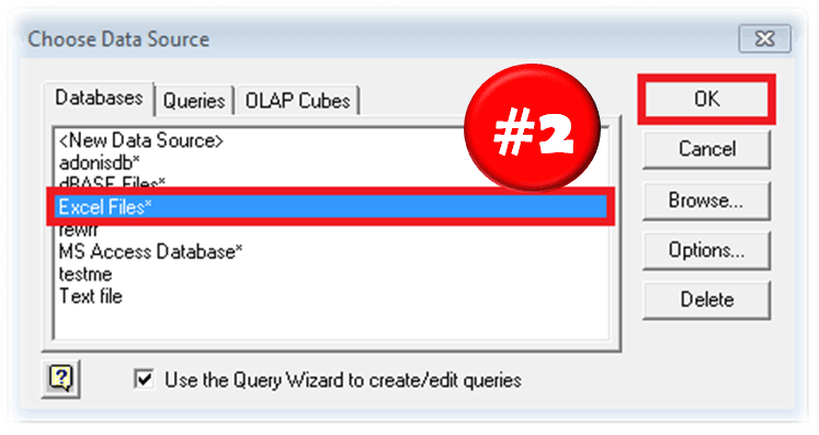 Next we need to specify the Data Source for our Microsoft Query. Select Excel Files to proceed.
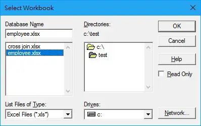
Select Excel Source File
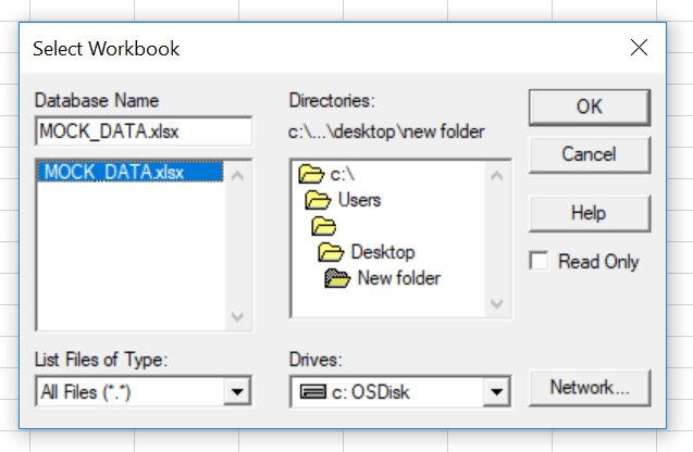 Now we need to select the Excel file that will be the source for our Microsoft Query. In my example I will select my current Workbook, the same from which I am creating my MS Query.
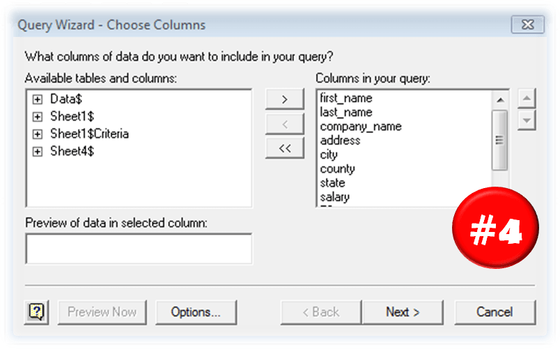
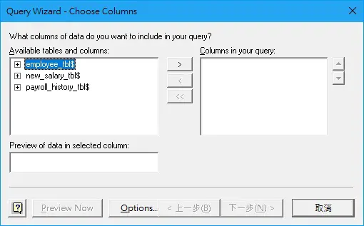
Select Columns for your MS Query
The Wizard now asks you to select Columns for your MS Query. If you plan to modify the MS Query manually later simply click OK. Otherwise select your Columns.
Return Query or Edit Query
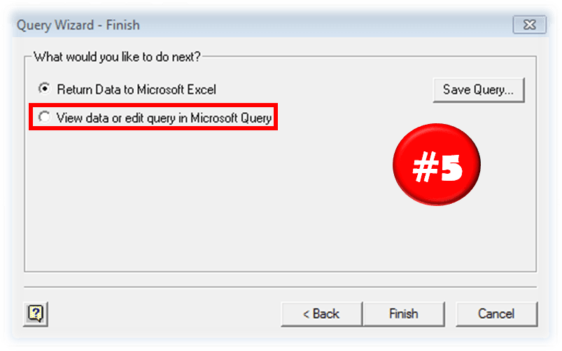 Now you have two options:
- Return Data to Microsoft Excel – this will return your query results to Excel and complete the Wizard
- View data or edit query in Microsoft Query – this will open the Microsoft Query window and allow you to modify you Microsoft Query
Optional: Edit Query
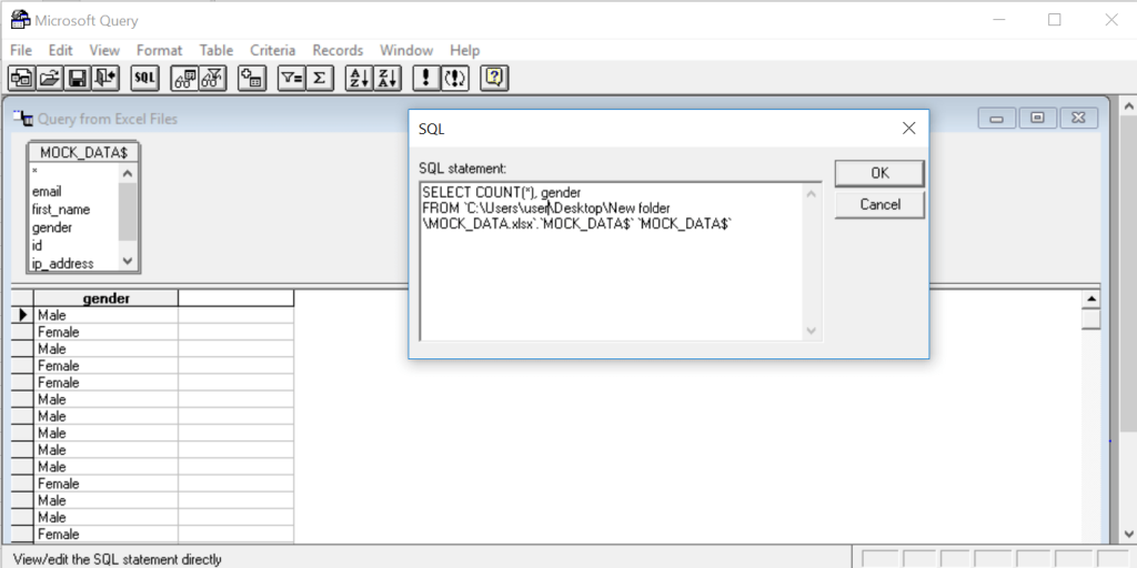 If you select the View data or edit query in Microsoft Query option you can now open the SQL Edit Query window by hitting the SQL button. When you are done hit the return button (the one with the open door).
Import Data
When you are done modifying your SQL statement (as I in previous step). Click the Return data button in the Microsoft Query window.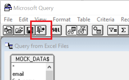
This should open the Import Data window which allows you to select when the data is to be dumped.
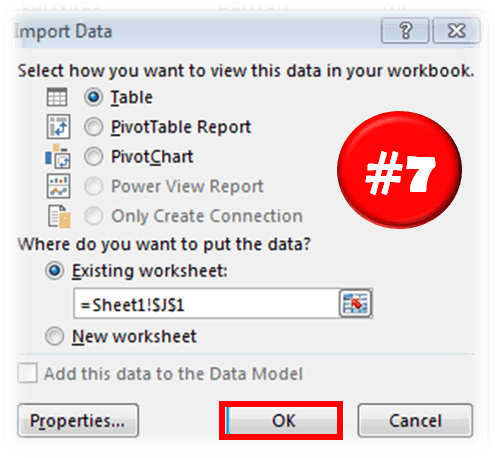 Lastly, when you are done click OK on the Import Data window to complete running the query. You should see the result of the query as a new Excel table:
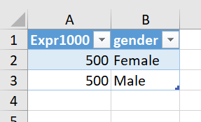
As in the window above I have calculated how many of the records in the original table where Male and how many Female.
AS you can see there are quite a lot of steps needed to achieve something potentially pretty simple. Hence there are a couple of alternatives thanks to the power of VBA Macro….
MS Query – Create with VBA
If you don’t want to use the SQL AddIn another way is to create these queries using a VBA Macro. Below is a quick macro that will allow you write your query in a simple VBA InputBox at the selected range in your worksheet.
Just use my VBA Code Snippet:
Sub ExecuteSQL()
    Attribute ExecuteSQL.VB_ProcData.VB_Invoke_Func = "Sn14"
    'AnalystCave.com
    On Error GoTo ErrorHandl
    Dim SQL As String, sConn As String, qt As QueryTable
    SQL = InputBox("Provide your SQL Query", "Run SQL Query")
    If SQL = vbNullString Then Exit Sub
    sConn = "OLEDB;Provider=Microsoft.ACE.OLEDB.12.0;;Password=;User ID=Admin;Data Source=" & _
        ThisWorkbook.Path & "/" & ThisWorkbook.Name & ";" & _
        "Mode=Share Deny Write;Extended Properties=""Excel 12.0 Xml;HDR=YES"";"
    Set qt = ActiveCell.Worksheet.QueryTables.Add(Connection:=sConn, Destination:=ActiveCell)
    With qt
        .CommandType = xlCmdSql
        .CommandText = SQL
        .Name = Int((1000000000 - 1 + 1) * Rnd + 1)
        .RefreshStyle = xlOverwriteCells
        .Refresh BackgroundQuery:=False
    End With
    Exit Sub
ErrorHandl: MsgBox "Error: " & Err.Description: Err.Clear
End Sub
Just create a New VBA Module and paste the code above. You can run it hitting the CTRL+SHIFT+S Keyboardshortcut or Add the Macro to your Quick Access Toolbar.
Learning SQL with Excel
Creating MS Queries is one thing, but you need to have a pretty good grasp of the SQL language to be able to use it’s true potential. I recommend using a simple Excel database (like Northwind) and practicing various queries with JOINs.
Alternatives in Excel – Power Query
Another way to run queries is to use Microsoft Power Query (also known in Excel 2016 and up as Get and Transform). The AddIn provided by Microsoft does require knowledge of the SQL Language, rather allowing you to click your way through the data you want to tranform.
MS Query vs Power Query Conclusions
MS Query Pros: Power Query is an awesome tool, however, it doesn’t entirely invalidate Microsoft Queries. What is more, sometimes using Microsoft Queries is quicker and more convenient and here is why:
- Microsoft Queries are more efficient when you know SQL. While you can click your way through to Transform Data via Power Query someone who knows SQL will likely be much quicker in writing a suitable SELECT query
- You can’t re-run Power Queries without the AddIn. While this obviously will be a less valid statement probably in a couple of years (in newer Excel versions), currently if you don’t have the AddIn you won’t be able to edit or re-run Queries created in Power Query
MS Query Cons: Microsoft Query falls short of the Power Query AddIn in some other aspects however:
- Power Query has a more convenient user interface. While Power Queries are relatively easy to create, the MS Query Wizard is like a website from the 90’s
- Power Query stacks operations on top of each other allowing more convenient changes. While an MS Query works or just doesn’t compile, the Power Query stacks each transform operation providing visibility into your Data Transformation task, and making it easier to add / remove operations
In short I encourage learning Power Query if you don’t feel comfortable around SQL. If you are advanced in SQL I think you will find using good ole Microsoft Queries more convenient. I would compare this to the Age-Old discussion between Command Line devs vs GUI devs…
26 Sep ’22 by Antonio Nakić-Alfirević
SQL Query function in Excel
If you’re reading this article you probably know that Google Sheets has a QUERY function that allows you to run SQL-like queries against data in the sheet. This function lets you do all sorts of gymnastics with the data in your sheet, be it filtering, aggregating, or pivoting data.
Being a fully-fledged desktop app, Excel tends to be more feature-rich than Google Sheets. This is especially true in the data analytics department where Excel shines with advanced Excel functions as well as Power Query functionality.
However, Excel doesn’t natively have a QUERY function that you can use in cells on the sheet.
In this blog post, I’m going to show you how to add a QUERY function to Excel and give a few examples of how to use it.
First look
Let’s start by taking a look at the function in action.

The function is pretty straightforward. It accepts the SQL query as the first parameter and returns a table with the results of the query.
The results automatically spill to the necessary amount of space. This spilling behavior relies on the dynamic array functionality that’s available in Excel 365 (but isn’t in earlier versions of Microsoft Excel).
Works with Excel tables
In Google Sheets, the QUERY function references data by address (e.g. “A1:B10”) while columns are referenced by letters (e.g. A, B, C…).
This works but has some drawbacks:
- It makes the query sensitive to the location of the data. If the data is moved or if columns are reordered, the query will break.
- It makes the query difficult to read since it uses range addresses and column letters instead of table and column names (e.g. Employees, DateOfBirth…)
- Adding or removing rows can break the query. For example, if the provided range is “A1:H10” the query will only take into account the first 10 rows. If additional rows are added, the query will not take them into account. You can get around this by omitting the end row number (e.g. “A1:H”), but this means that there must be no other content below the data range.
Excel, on the other hand, allows explicitly defining tables (aka ListObjects) that delineate the areas that hold data. Each Excel table has a name, as do its columns. This makes Excel tables very similar to database tables and makes them easier to work with from SQL.

Full SQL syntax support (SQLite)
Under the hood, the Windy.Query function is powered by SQLite – a small but powerful embedded database engine.
When called, the function passes the query to the built-in SQLite engine which has an adapter that lets it use Excel tables as its data source.
This means that the entire SQLite syntax is available for use in queries. In comparison, in Google Sheets, the query syntax is rather limited. It only supports a single table (no joins) and a very small set of built-in functions.
Examples of use
Since the engine under the hood is SQLite, queries can use all operations available in SQLite, including table joins, temp tables, column table expressions, window functions etc… Let’s go over some examples of how to use these in Excel.
Joining tables
Here’s an example of a simple one-to-many join:

The usual way of doing a simple operation such as this one in Excel would be to use xlookup or PowerQuery, but SQL is now another option. And if we needed anything more complex than a simple join, SQL would quickly shine as the most powerful and convenient option of the three.
Merging table rows (union)
Another way we might want to combine two (or more) tables is to combine their rows. We can do this with a SQL UNION operator.
The tables might have some rows in common. If we want to keep only one instance of such rows we would use the regular UNION operator. If we want to keep both versions of rows that are in common, we would use the UNION ALL operator.

Finding differences between two tables
In the previous example, we had two tables that had some rows in common and some rows not. Let’s assume, for example, that the first table contains last year’s list of employees and the second table is the new list of employees.
If we wanted to find out the differences between the two tables, we could easily do that with a bit of SQL.
All of the rows that are in the first table but not in the second one we will mark as “deleted”. All of the rows that are in the second table but not in the first one we will mark as “added”. Here’s what that SQL query looks like:
select
	id, name, 'deleted'
from
	employees e where not exists (select * from Employees_New en where e.id == en.Id)
union
select
	id, name, 'added'
from
	employees_new en where not exists (select * from Employees e where e.id == en.Id)
And here’s what the result looks like:

Ranking rows
Another useful thing we might want to do is rank rows based on some criteria. For example, suppose we have a table with a list of cities. For each city we have its population and the country it belongs to.
Our task is to find the top 3 cities in each country based on population. Here’s how we might do that in SQL.
-- we use this CTE so we can reference the calculated 'rank_pop' column in the where clause
with cte as (
	select
		city,
		country,
		population,
		-- using the RANK() window function
		RANK() OVER (PARTITION BY country ORDER BY population) as rank_pop
	from
		cities c)
select
	*
from
	cte
where
	-- filtering by the 'rank_pop' column from the CTE
	rank_pop <= 3
order by country, rank_pop

This query is a bit more complex than the previous ones. It uses a common table expression and a window function (the rank function), and showcases the ability to write complex SQL in queries.
Queries can also make use of dozens of built-in SQLite functions. Various specialized extended functions such as RegexReplace, GPSDist (GPS distance between two points) and LevDist (fuzzy text matching) are also available.
Updating tables
OK, this next example is a bit of a hack, but a useful one… The query you supply doesn’t need to be a SELECT query. You can do UPDATE/INSERT/DELETE statements as well, and these will modify the data in the target Excel tables.

This can be a handy way to clean and transform data in your tables in place, without having to export/import the data to an external database (e.g. SQL Server, MySql, Postgres…).
This works because the SQLite engine isn’t copying the data. Rather, it’s using an adapter that lets it access live data in the Excel table.
How does the function see Excel tables?
At first glance, it might seem strange that the query can access your workbook tables. After all, we did not pass them in as parameters, and functions normally only work with parameters that are passed to them.
However, the Windy.Query function is aware of the workbook it’s being called from and it can read data from the workbook’s tables without the need for passing them in as parameters. This makes the function much easier to call especially when working with multiple tables.
Column Headers
Results returned by the Windy.Query function can optionally include headers. This is controlled by the second parameter of the function.

The texts in the column headers are determined by the SQL query itself. You can easily rename result columns by aliasing them in the select list.

Automatically refresh results
By default, the SQL query runs as a one-off operation when you enter the formula but does not refresh if the source tables change. However, if you want the query to refresh whenever one of the source tables changes, you can easily do so by setting the autoRefresh argument to true.

Note that the auto-refresh functionality relies on Excel’s RTD (Real-Time Data) server. The RTD server usually throttles updates so functions don’t overwhelm Excel with frequent updates. The default throttle interval is 2s meaning that the function will not update more than once every 2s. To improve responsiveness, you can lower this value to something like 20ms. The simplest way to do this is through the “Configure” dialog in the QueryStorm runtime’s ribbon.

Passing parameters
When needed, SQL queries can use values from cells as parameters. To use a cell as a parameter in a query, start by giving the cell a name (named range).

Once the cell has a name, you can reference it in the query using the @paramName or $paramName syntax.

If automatic refresh is turned on, results will automatically refresh whenever one of the parameter cells changes its value.

Performance
This is all well and good for small tables, you might think, but how does it handle large data sets? Well, it handles them quite well. The function can read source tables of 100k rows and 10 columns within a few milliseconds and can return this amount of data in a second or two. In addition to this, all columns are automatically indexed so searches and joins are extremely performant as well.
This makes the function perform very well, both from the data throughput standpoint as well as from the computational one.
OK, so is this better than the Google Sheets version of the QUERY function?
Yes, dah. Did you read the previous chapters? 😛
Installing the Windy.Query function
So how do you install this function into your Excel? It’s a simple 2-step process.
Step 1 is to install the QueryStorm Runtime add-in (if you don’t already have it). This is a free, 4MB add-in for Excel that lets you install and use various extensions for Excel. It’s basically an app store for Excel.
Step 2 is to click the “Extensions” button in the “QueryStorm” tab in the Excel ribbon, find the Windy.Query package in the “Online” tab, and install it.

What happens if I share the workbook with a user who doesn’t have the function?
Nothing bad. If the other user doesn’t have the function installed, they will see the last results of the query that were returned on your machine. They just won’t be able to refresh the results.
Advanced SQL query editor
Writing SQL queries in the formula bar can get a bit unwieldy. To make queries easier to write, it’s better to use a proper editor, preferably one that offers syntax highlighting and code completion for SQL and knows about the tables in your workbook.
For this purpose, I recommend using the QueryStorm IDE. This is an advanced IDE that lets you use SQL in Excel. You can write the query in the QueryStorm code editor and then paste the query into the Windy.Query function when you’re happy with it (if needed).

The IDE does more than just allow using SQL in Excel. You can use it to create and share functions and addins for Excel. In fact the QueryStorm IDE was used to create the Windy.Query function itself.
The IDE has a free community version for individuals and small companies, while users in larger companies can make use of the free trial license. For paid licenses, check out the pricing page.
You can read more in this blog post that’s dedicated to the QueryStorm SQL IDE.
Video demonstration
For a video demonstration of the Windy.Query function, take a look the following video:
This Microsoft Excel tutorial explains how to create Excel Query, create Join Table, update Query, add Query criteria.
You may also want to read:
Excel automatically select specific columns using Custom Views and Query
Microsoft Excel create Query
Similar to Microsoft Access Query, Excel allows users to create Query through graphical user interface, which means you don’t need to have technical skills to write any SQL statement. Although Microsoft Excel has the capability to do that, Access undeniably provides a much easier way to build Query because
- You can create Expression and apply criteria on it
- You can create SubQuery
- You can build many different relationships with different types of Joins in a single Query
Therefore, if you really want to build complicated Query, you should use Access to link table back to Excel data.
To begin, navigate to Data > From Other Sources > From Microsoft Query

Select Excel Files > OK
Select the workbook that contains the data. You can select Workbook that you are currently opening > OK
Select the worksheet, and then add the fields you need to the right panel (click on the arrow in the middle)
If you cannot see the Worksheet names, click on Options button and check System Tables check box.
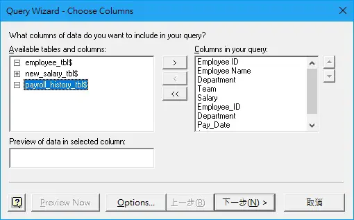
In this example, I have selected all the fields under worksheet employee_tbl and payroll_history_tbl. Click on Next.
The below message box pops up saying you have to join the Table by yourself. It doesn’t matter because I don’t want Excel to guess what I want to join.

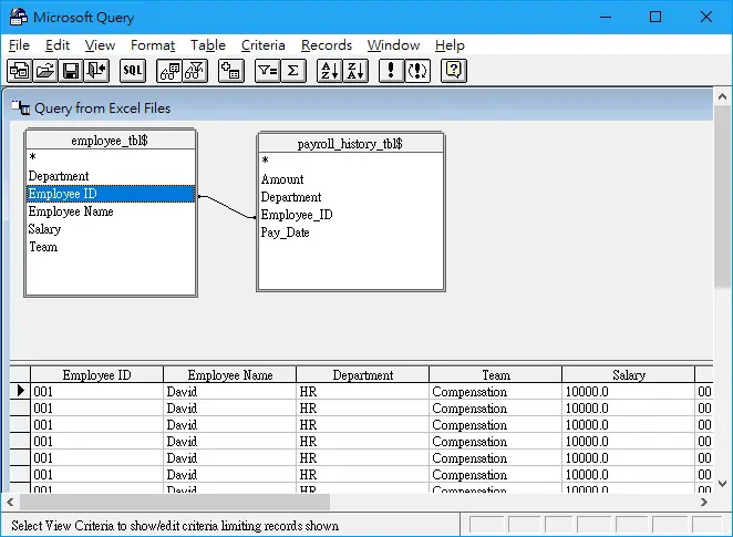
Because Employee ID is the only key in these two Table, I drag the Employee ID field of one Table to Employee ID field of the other Table in order to create an Inner Join.
The result is immediately displayed in the lower table.
In the previous step, I have selected all the fields from two Tables, therefore some fields such as Employee ID and Department are duplicated. Highlight the fields you want to remove from the result, click on Delete button on the keyboard.

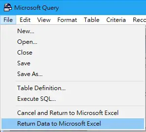
To return Query result, navigate to File > Return Data to Microsoft Excel
Select a Cell you want to return data > OK

Now data is returned. When the data source is updated, you can refresh this table by clicking Data tab > Refresh All

Edit Excel Query
To edit Excel Query, right click on the Table in the worksheet > Table > Edit Query
Go through the Wizard Query to select fields > add criteria > sort data > edit Query
Alternatively, cancel the Wizard Query to directly jump to the Query view.
Add Table and Delete Table in Excel Query
It is possible to join additional tables from another source (must be under the same folder, same file type) by clicking on the Add Table button in the tool bar.

However, if you have more than 2 Tables, you cannot create Left Join or Right Join, you can only create Inner Join.
To delete a Table, click on t he Table and press the Delete button on your keyboard.
Add Criteria to Excel Query
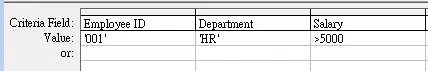
To Add criteria, click on the Show/Hide Criteria button in the tool bar, select the Criteria Field and enter a Value.

If you have more than one criteria, type all criteria in the same Value row if they are AND condition.
Type all criteria in different Value row if they are OR condition.

Create Right Join and Left Join
By default, when you drag one field from one Table to another field, the relationship built is Inner Join (return result where both keys are matched).
Instead of creating Inner Join, you can double click on the relationship line to open the Joins dialog.
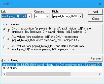
The first option is Inner Join, 2nd option is Left Join, 3rd option is Right Join.
For Inner Join, the relationship line is a straight line without any arrow.
For Left Join, the relationship line will show an arrow pointing from table that includes all fields to another table.
For Right Join, the relationship line will show an arrow pointing to table that includes all fields from another table.
Select an option, then Click on Add button, the SQL statement in the lower box will update accordingly, press Close button to finish editing.
07 Aug 3 Ways to Perform an Excel SQL Query
Posted at 12:08h
in Excel VBA
0 Comments
Howdee! Excel is a great tool for performing data analysis. However, sometimes getting the data we need into Excel can be cumbersome and take a lot of time when going through other systems. You’re also at the mercy of how a disparate system exports data, and may need an additional step between exporting and getting the data into the format you need. If you have access to the database where the data is housed, you can circumvent these steps and create your own custom Excel SQL query.
To follow along with my below demos, you’ll need to have an instance of SQL server installed on your desktop. If you don’t, you can download the trial version, developer version, or free express version here. I’ll be working with the free developer version in this article. I’m also using a sample database that you can download here. The easiest way to install this is using SQL Server Management Studio (SSMS). That download is available here. Once you open SSMS, it should automatically detect your local server instance. You must ensure your SQL Server User is running as the “Local Client” and then you can create a blank database, and restore that database from the backup file. If you have issues accomplishing this, let me know in the comments and I’ll elaborate on how this is done.
If you are familiar enough with SQL and have access to your own data, you can skip these steps and use your data. Otherwise, I recommend downloading these tools before getting started. If you’re new to SQL, I highly recommend the SQL Essential Training courses on Lynda.com. Now, on to why you’re all here…
Excel SQL Query Using Get Data
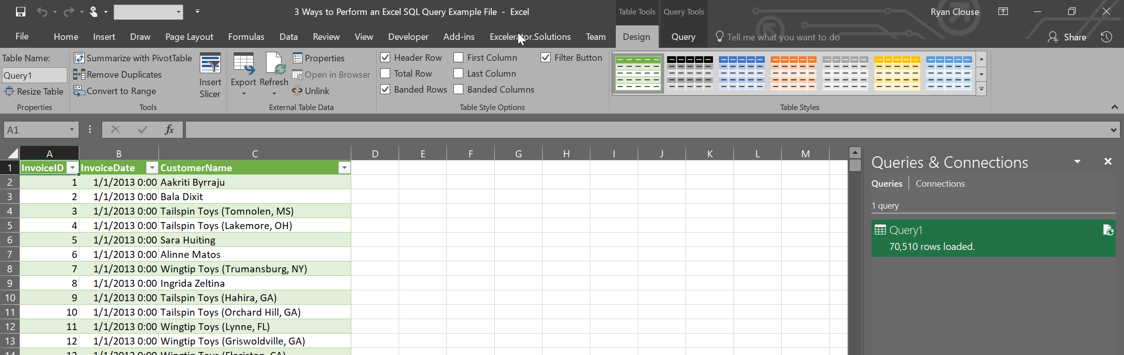
This option is the most straight forward approach to creating an Excel SQL query. However, it is important to note that this approach is only available in Excel 2013 and later and will not currently work on Mac OSX. To get started, select “Get Data” à “From Database” à “From SQL Server Database” as shown in the screen grab. At this point it will pop-up a prompt to enter your server name and the target database you’re wanting to query (you can get this information from SSMS). You can enter this information and then select “OK”. This will allow you to browse available tables from that database to import. You can remove columns and filter tables before importing. If you do not know how to write SQL queries yet, this is one approach you can take.
However, if you select the “Advanced” dropdown arrow, you can create your own custom Excel SQL query. I usually create my query in SSMS or Visual Studio and then just paste the final query in this window. That is because there is no intellisense in this window and it can be difficult to spot errors in your query. Once you select OK, it will ask you to confirm credentials and you may get an error about encryption. This is common when connecting to databases in this manner and nothing to worry about. The next screen will provide an example of your data and you can select “Load” to import it.

This will create a table on a new tab and you’ll also notice a new pane on the right titled “Connections & Queries”. It will display the name of your query (defaults to “Query1”, “Query2”, etc.) and you can rename the query by right-clicking and selecting “Rename”. You can also edit the query from this location as well. It will open up an interface with a sample of your data and you can add/remove columns, filter your data, or edit your source query from here.
Now that you’ve set up this Excel SQL query, you can simply refresh the data set with fresh data anytime by clicking “Refresh All” on the “Data” ribbon. A quick side note here. If you pivot this data, “Refresh All” will refresh pivot tables first and then the query. To update your pivot table, you’ll need to refresh all twice or update your pivot table manually. To me, one of the downsides of this approach is the results are always returned in a table. I personally do not like working with tables in Excel. That’s where using VBA for your SQL query can come in handy.
Excel SQL Query Using VBA
Using VBA to create your Excel SQL query is not as straight forward as the previous approach, but can still be an extremely useful method depending on your situation. I particularly like that the data is not returned to a table unless you designate it to be so. This technique will work on older versions of Microsoft Excel but will not work on Mac OSX versions of Excel since it uses and ADO connection.
To get started, open up the VBA editor by pressing alt+F11. Before beginning to write your code, you’ll need to ensure that the “Microsoft ActiveX Data Objects 2.0 Library” is referenced from the VBA Project. To do this, click on “Tools” in the ribbon menu at the top of the VBA editor. In the popup, ensure the library is checked as shown below. This allows the project to use the ADO connectors to create the connection to your database. Next, let’s dimension a few variables.

Dim Conn As New ADODB.Connection
Dim recset As New ADODB.Recordset
Dim sqlQry As String, sConnect As String
The Conn variable is will be used to represent the connection between our VBA project and the SQL database. The receset variable will represent a new record set through which we will give the command to perform our Excel SQL query using the connection we’ve established. Finally, the sqlQry variable will represent a string variable that is our SQL query command, and the sConnect variable will be a string representing the connection string the database requires. Let’s look at how to use these variables to perform a SQL query.
sqlQry = "select top 1000 si.InvoiceID, si.InvoiceDate, sc.CustomerName from Sales.Invoices si" & _
             " left join sales.Customers sc on sc.CustomerID = si.CustomerID"

sConnect = "Driver={SQL Server};Server=[Your Server Name Here]; Database=[Your Database Here];Trusted_Connection=yes;"

Conn.Open sConnect

Set recset = New ADODB.Recordset

    recset.Open sqlQry, Conn
    Sheet2.Cells(2, 1).CopyFromRecordset recset
    recset.Close

Conn.Close

Set recset = Nothing
While this may look complex, each step is relatively simple. Firstly, we set our sqlQry variable equal to a string that represents the syntax of our SQL query. We then create a connection string we can use in our next command to connect to the database. So, “Conn.Open” is the command to open the connection and “sConnect” is the string it uses to do so. “Trusted_Connection=yes” means that the connection will attempt to be established using your Microsoft credentials for the account you’re logged in as.
Now that the connection is open, we can open a new record set and pass it the sql command using the sqlQry variable, and tell it which connection to use by passing it the Conn variable. We can then use the VBA command “CopyFromRecordset” to paste the recordset anywhere in our workbook. It’s important to close both the record set and connection at this point. You also want to set your recset variable equal to nothing so it does not eat up valuable resources.
One of the downsides to using this method is that you must explicitly tell Excel some things that the previous approach did automatically. For example, this SQL query will not return any column headers. Therefore, you must explicitly tell Excel what to label your columns. Secondly, the data is not automatically cleared and the new query imported. You must also explicitly tell Excel to do this as well. Here is the final code with those commands added.
Sub SQL_Example()
Dim Conn As New ADODB.Connection
Dim recset As New ADODB.Recordset
Dim sqlQry As String, sConnect As String

Sheet2.Cells.ClearContents

sqlQry = "select top 1000 si.InvoiceID, si.InvoiceDate, sc.CustomerName from Sales.Invoices si" & _
            " left join sales.Customers sc on sc.CustomerID = si.CustomerID"

sConnect = "Driver={SQL Server};Server=[Your Server Name Here]; Database=[Your Database Name Here];Trusted_Connection=yes;"

Conn.Open sConnect
Set recset = New ADODB.Recordset

    recset.Open sqlQry, Conn
    Sheet2.Cells(2, 1).CopyFromRecordset recset
    recset.Close

Conn.Close
Set recset = Nothing

Sheet2.Cells(1, 1) = "Invoice ID"
Sheet2.Cells(1, 2) = "Invoice Date"
Sheet2.Cells(1, 3) = "Customer Name"

End Sub
My preference for using this approach is when I want the user to be able to pass parameters to my Excel SQL query. For example, I might have a dropdown of customer names the user could select. By using this tactic, I can easily add a dropdown of customer names the user can select, and pass that value to my SQL query in a where clause.
As you can see, both the built in Excel SQL query and the VBA method have pros and cons. I employ both in my everyday work depending on what situation I find myself in.
Excel SQL Query Using Microsoft Query
This option is likely the most complex option, but it has the added advantage of being compatible with some versions of Mac OSX. I won’t pretend to be an expert at creating Mac OSX compatible tools for Excel, but I have successfully used this implementation to create an embedded Excel SQL query for Macs in the past.
I also like this method because you can create popup style parameters. For example, you can prompt the user to input date range parameters at the time the SQL query is ran. Like the first example, running this query is as easy as clicking “Refresh All” on the Data ribbon. Let’s dive in to the details.
To get started here, click “Get Data” on the Data ribbon. In the menu that dropdowns select “From Other Sources” and, finally “From Microsoft Query”.

This will open a wizard for you to choose your data source. Double click “<New Data Source>” and you’ll be prompted to enter some information about your data source. Option 1 can be anything you wish that describes your data source. Option 2 should be “SQL Server”. Click “Connect” and it will pop up a third window where you can enter information about the server and login information. Be sure you select the “Options>>” dropdown so you can select the database you’re wanting to connect to.

You’ll now have a new data source in the original window. Double click the data source to bring up a table import wizard. If you want to import an entire table, you can do so here and even filter and sort the data using the import wizard. However, if you want to use your own custom query as we have been, just select any field and go through the wizard and import the data. When you come to screen that asks you if you want to return the data to Excel or edit in a query, return the data to Excel. It will then prompt you to select where you want the data returned in your workbook.
The query will return the data in a table format. To change it to your own custom SQL query, let’s follow these steps:
- Click anywhere in the data table.
- On the Excel Data Ribbon, in the “Queries & Connections” group, properties will no longer be grayed out like it normally is. Click this.
- In the popup – you’ll see another properties icon. Click this.
- In this popup, select the “Definition” tab and paste your SQL query in the “Command Text” input box.
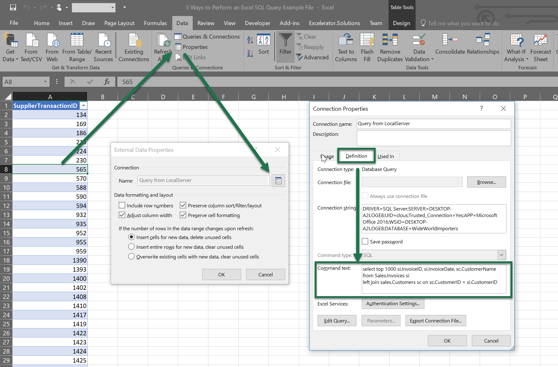
Now you’ve built an Excel SQL Query that can be refreshed anytime the workbook is refreshed. In my screengrab, the “Parameters” button is greyed out. If you want to add parameters to your query, you do so by adding “?” in your command text. That looks like this.
This creates a parameter the end user can interact with. You can have the user be prompted to enter an input when the workbook is refreshed, select a default value, or have it linked to a cell in the workbook. Even though this option is cumbersome to set up, I really enjoy using it. It allows me a lot of flexibility to have the user interact with the data. As I touched on in the beginning, I’ve had success using this option on Microsoft Office for Mac OSX. I don’t want to say this will work 100% of the time on a Mac because I’ve also had it fail. If anyone has any input on this, I’d love to hear from you.
Let me know your thoughts on these approaches in the comments! What other ways do you creatively get data into Excel from SQL data sources?
Cheers!
R