
Excel – довольно удобный инструмент с обширным функционалом. Множество приложений предлагают возможность создавать различные списки, но зачем пользоваться другими программами, если есть Excel?

♥ ПО ТЕМЕ: Экспозиция фокуса в «Камере» iPhone: настройка и фиксация.
Ниже мы покажем, как создать таблицу с флажками, которые вы можете удалять по мере выполнения задач. Excel даже отобразит, когда вы снимете все флажки. Создать таблицу довольно просто. Для этого нужно открыть вкладку «Разработчик», внести список задач, добавить флажки и расширенное форматирование. А теперь по порядку.
♥ ПО ТЕМЕ: Таблицы в Заметках на iPhone, iPad и Mac (macOS): как создавать и настраивать.
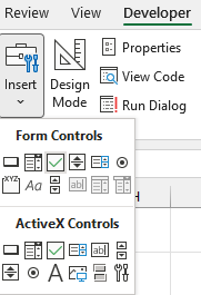
1. Открыть вкладку «Разработчик»
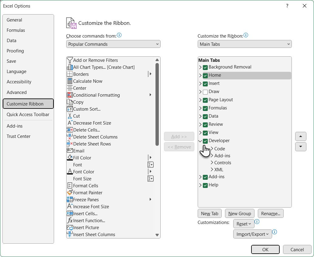
По умолчанию вкладка «Разработчик» не отображается. Ее можно добавить в ленту следующим образом: откройте «Файл» → «Параметры» → «Настроить ленту». В списке «Основные вкладки» установите флажок «Разработчик», а затем нажмите «Готово».

♥ ПО ТЕМЕ: «Правило третей» при съемке с помощью iPhone: что это и как использовать.
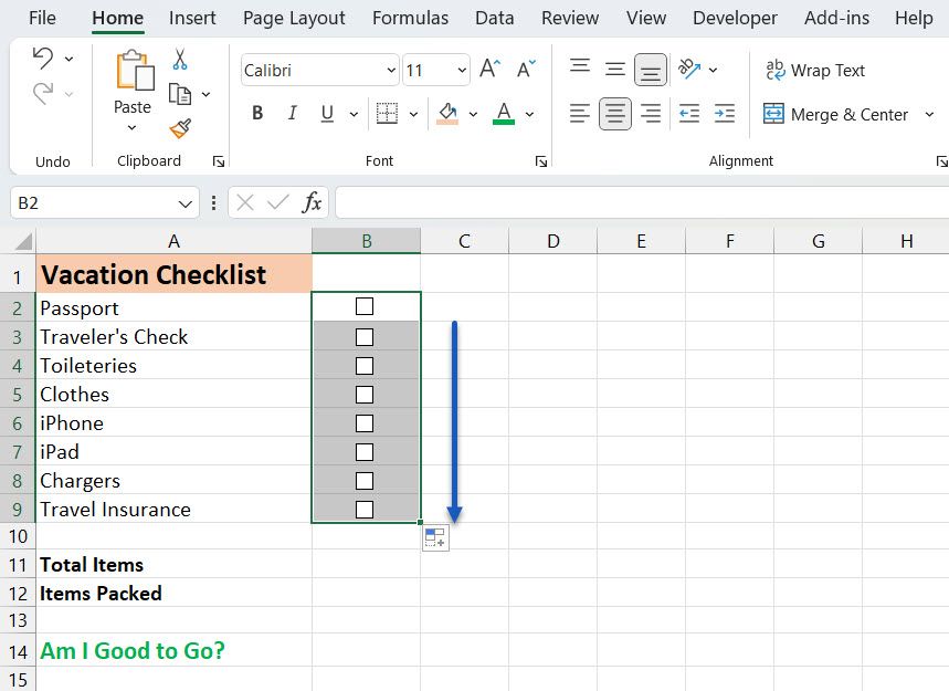
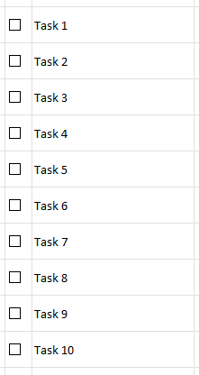
2. Добавление списка задач в таблицу
В каждой ячейке таблицы укажите задачу. В нашем примере одна из ячеек будет содержать «Общее количество предметов», вторая – «Упакованные предметы». Ячейка «Я готов» будет отображаться красным, если не все галочки в списке сняты, и зеленым, если флажки сняты все.
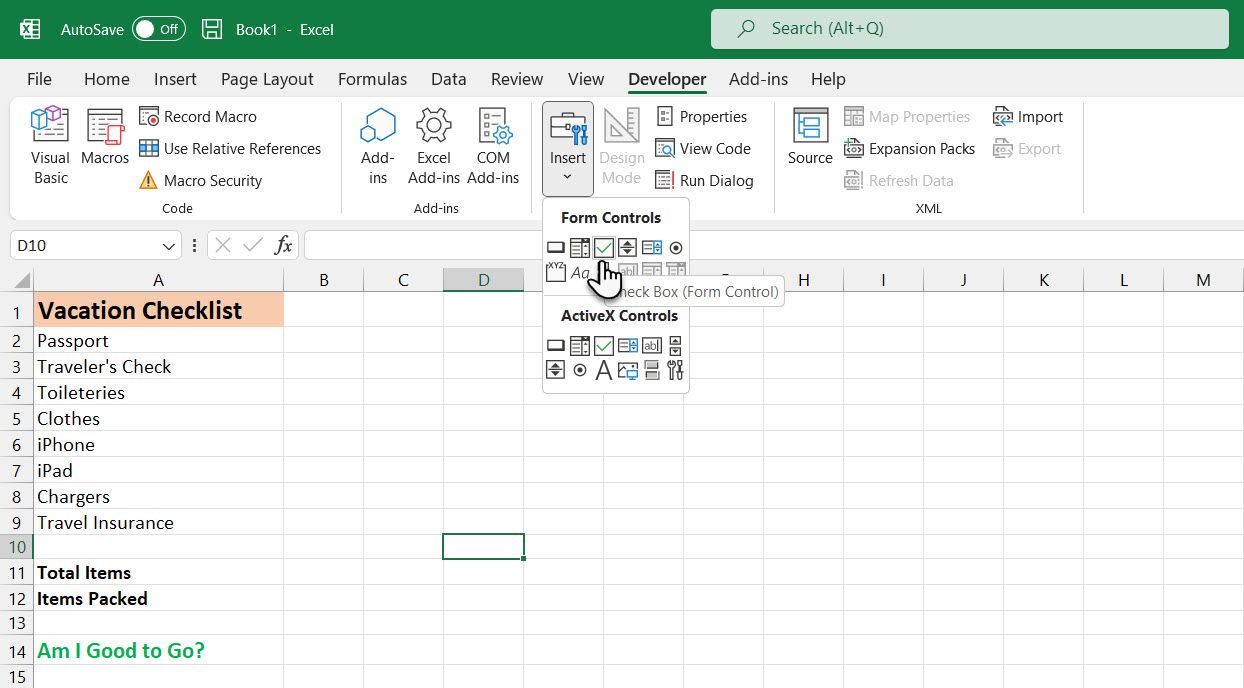
Откройте вкладку «Разработчик». Нажмите «Вставить» и в разделе «Элементы управления формы» выберите «Флажок» (иконку с галочкой).

♥ ПО ТЕМЕ: Как удаленно подключиться к iPhone или iPad и просматривать его экран с компьютера, Android или iOS-устройства.
3. Добавление флажков
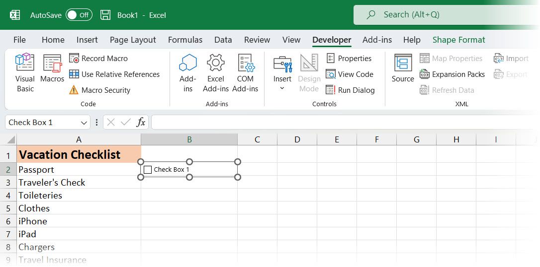
Кликните на ячейку, в которую хотите добавить флажок. Вы увидите, что справа от поля флажка отображается текст. Так как нам нужно только поле, выделите текст и удалите его. После удаления текста размер поля не изменяется автоматически.

Если вы хотите изменить его, щелкните правой кнопкой мыши по ячейке, чтобы выбрать поле, а затем левой кнопкой мыши щелкните по нему. Таким образом вы сможете изменить его размеры и переместить на середину ячейки. Для того чтобы скопировать поле флажка и разместить его в других ячейках, выберите ячейку, а затем используйте кнопки управления курсором (клавиши со стрелками на клавиатуре) для перемещения к ячейке с флажком. Для того чтобы скопировать поле флажка в другие ячейки, наведите курсор в нижний угол ячейки, захватите его кнопкой мыши и протяните по ячейкам, в которые нужно скопировать поле. Отпустите кнопку мыши.

♥ ПО ТЕМЕ: Gmail-мастер, или как навести порядок в почтовом ящике Google: 5 советов.
Расширенное форматирование списка
В зависимости от предназначения списка вы можете использовать расширенное форматирование.
Создание столбца ИСТИНА/ЛОЖЬ
Для этого нужно использовать колонку справа от полей с флажками. Флажок будет возвращать ИСТИНА (если галочка установлена) или ЛОЖЬ (если она снята). Таким образом вы сможете увидеть, все ли флажки сняты.
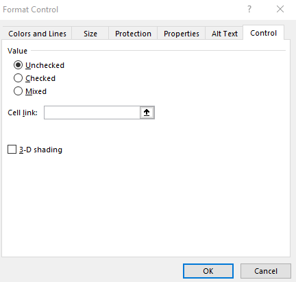
Правой кнопкой мыши нажмите на первое поле флажка и выберите «Формат объекта».

На вкладке «Элемент управления» в окне «Формат объекта» нажмите на кнопку выбора ячейки с правой стороны поля «Связь с ячейкой».

Выберите ячейку, которая находится справа от клетки с флажком. Адрес выбранной ячейки размещен в поле «Связь с ячейкой» в компактной версии окна «Формат объекта», чтобы развернуть его повторно нажмите на кнопку «Связь с ячейкой» и выберите «ОК». Повторите указанную процедуру для каждой ячейки в списке.

♥ ПО ТЕМЕ: Вибер для компьютера Windows, Linux и Mac на русском: восемь лайфхаков, которые вы могли не знать.
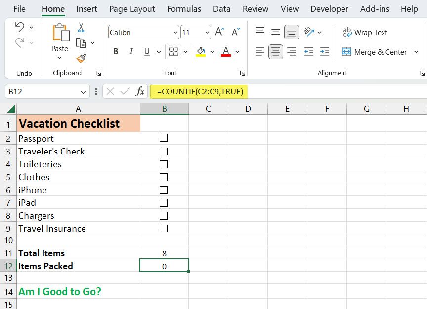
Общее число предметов и подсчет отмеченных предметов в списке
Укажите общее количество флажков в списке в ячейке, расположенной справа от клетки «Общее количество предметов». Число проставленных галочек можно подсчитать с помощью специальной функции. Введите
=СЧЁТЕСЛИ(C2:C8; ИСТИНА)
или
=COUNTIF(C2:C8,TRUE)
в ячейку справа от ячейки «Упакованные предметы» и нажмите Enter. Как показано в примере ниже, функция подсчитает число ячеек в колонке С (с С2 по С8), имеющих значение ИСТИНА или TRUE.

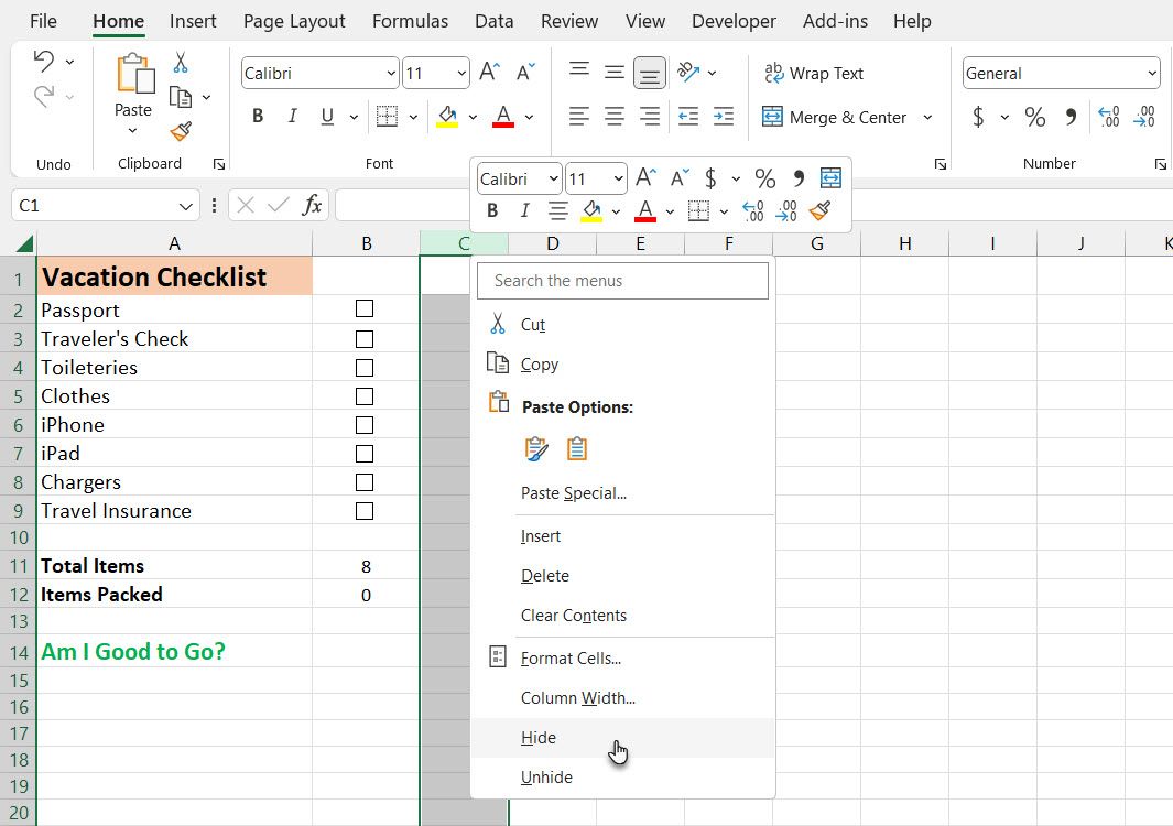
Скрыть столбец ИСТИНА/ЛОЖЬ
Для того чтобы скрыть данную колонку, правой кнопкой мыши кликните на ее заголовке и в отобразившемся меню выберите пункт «Скрыть». Столбец будет скрыт.

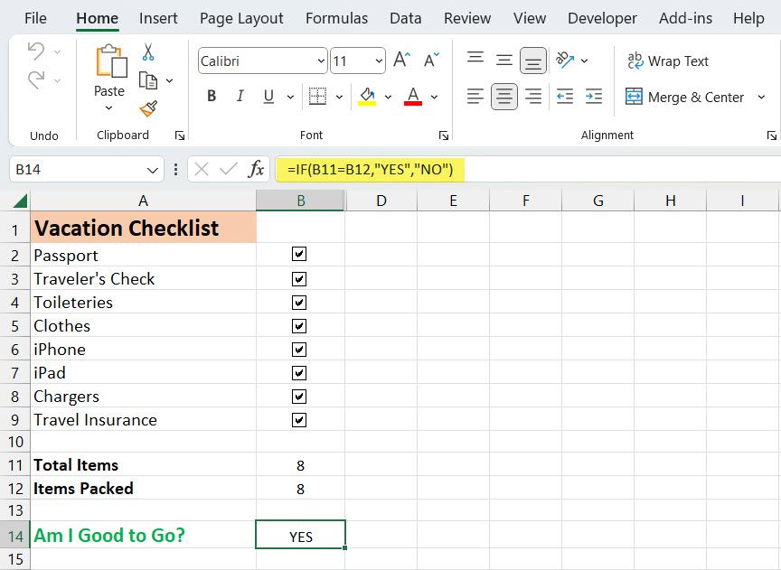
Как проверить, все ли галочки сняты
Для этого выберите ячейку «Я готов» и введите
=ЕСЛИ(B10=B11;"Да";"Нет")
или
=IF(B10=B11,"YES","NO")
Если число в ячейке В10 совпадет со значением подсчитанных флажков в ячейке В11, в ней автоматически отобразится «Да», в противном случае появится «Нет».

♥ ПО ТЕМЕ: Как хорошо выглядеть на любом фото: 5 простых советов.
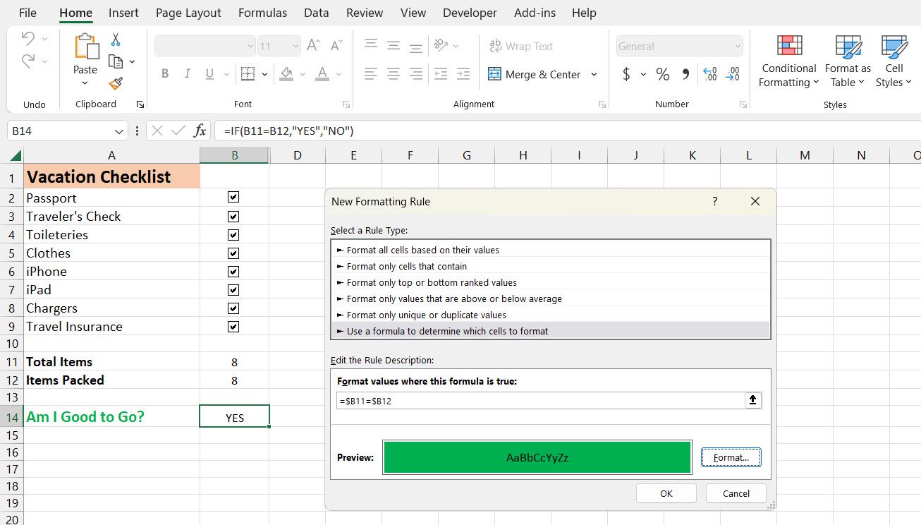
Применение условного форматирования
С помощью условного форматирования вы можете выделить ячейки цветом. К примеру, вы можете задать условное форматирование таким образом, чтобы все ячейки со значениями определенного типа закрашивались в красный цвет.
Создайте правило, открыв «Главная» → «Условное форматирование» → «Создать правило» → «Диспетчер правил условного форматирования» → «Использовать формулу для определения форматируемых ячеек». Введите
=$B10<>$B11
в поле «Форматировать значения, для которых следующая формула является истинной:». Замените значения В10 и В11 адресами ячеек «Общее количество предметов» и «Упакованные предметы», если это не одни и те же ячейки.

Создайте еще одно правило, но в поле «Форматировать значения, для которых следующая формула является истинной:» введите формулу
=$B10=$B11
Затем нажмите «Формат», выберите цвет и нажмите «ОК».
В окне «Диспетчер правил условного форматирования» введите адреса ячеек, которые должны быть заполнены цветом, в поле «Применяется к». Введите те же адреса для обоих правил. В нашем случае это =$B$13. Нажмите «ОК».

Ячейка «Я готов» окрасится зеленым цветом, если все галочки будут сняты, или красным, если нет.

Смотрите также:
- 3 бесплатных аналога Microsoft Office, с возможностью работы в «облаке».
- 10 полезных опций WhatsApp, которые следует знать каждому.
- Как закачать книги на iPhone и iPad бесплатно и без компьютера.
Many apps can create checklists, but do you need yet another app? For example, if you’re already using spreadsheets, you can easily make a checklist in Microsoft Excel.
Even if you don’t want to use it as a simple to-do list app, a checklist is an excellent way to track what you still need to do in your spreadsheet directly in the spreadsheet itself.
Let’s see how to create a checklist in Excel in five minutes or less.
How to Make a Checklist in Excel
We’ll show you how to create an Excel checklist with checkboxes you can tick off as you complete the items. It will indicate when you’ve checked off all the items so you can tell at a glance.
Here are the simple steps we’ll outline below:
- Enable the Developer Tab.
- Enter the checklist items into your spreadsheet.
- Add the checkboxes and advanced formatting.
1. Enable the Developer Tab
You must enable the Developer tab on the ribbon to create a checklist. To do this, right-click on the ribbon and select Customize the Ribbon.
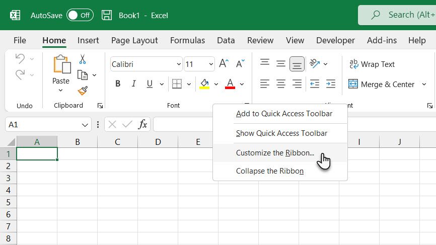
In the list of Main Tabs on the right side of the Excel Options dialog box, check the Developer box and click OK.
2. Enter the Checklist Items Into Your Spreadsheet
Enter your to-do list, one item per cell. In our example, we have a cell with the Total Items, and one with the total Items Packed, or how many items are checked off on our list.
The Am I good to go? cell will be red with NO if all the items are not checked off.
Once you check off all the items, the Am I good to go? cell turns green and will read YES.
Click the Developer tab. Then, click Insert in the Controls section and click the Check Box (Form Control).
3. Add the Checkboxes
Select the cell in which you want to insert the checkbox. You’ll see that there’s text to the right of the checkbox. We only want the text box, not the text. While the checkbox control is selected, highlight the text next to the checkbox, and delete it.
The checkbox control does not automatically resize once you’ve deleted the text. If you want to resize it, right-click on the cell to select the checkbox and then left-click on it (to make the context menu disappear). It will be selected with circles at the corners (as shown above).
Drag one of the circles on the right side towards the checkbox to resize the outline to just the size of the checkbox. Then, you can move the checkbox to the center of the cell with the four-headed cursor.
We want to copy that checkbox to the rest of our to-do list items.
To select the cell containing the checkbox, select any cell around it without a checkbox. Then, use one of the arrow keys on your keyboard to move to the cell with the checkbox.
To copy the checkbox to the other cells, move your cursor over the bottom-right corner of the selected cell with the checkbox until it turns into a plus sign. Make sure the cursor is NOT a hand. That will check the box.
Drag the plus sign down over the cells into which you want to copy the checkbox and release the mouse button. The checkbox is copied to all those cells.
Advanced Checklist Formatting
Depending on what you want to use your checklist for, you can add additional formatting elements to validate your list and display its status.
Create a True/False Column
For this step, we need to use the column to the right of the checkboxes to store the TRUE and FALSE values for the checkboxes. That allows us to use those values to test whether all the boxes are checked.
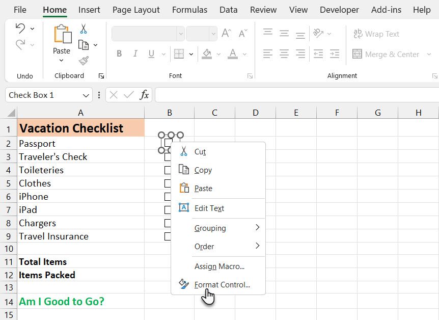
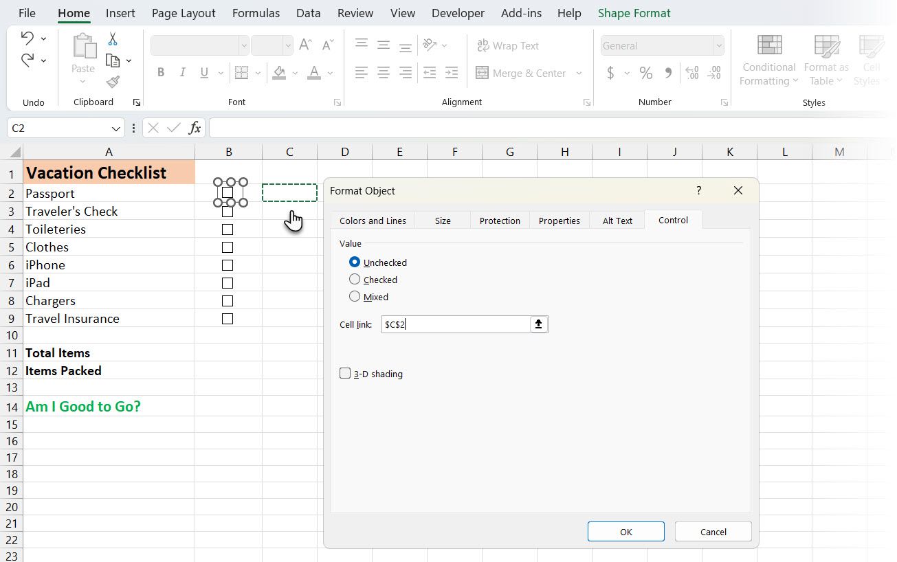
Right-click on the first checkbox (not the cell with the checkbox) and select Format Control.
On the Control tab on the Format Object dialog box, click the cell selection button on the right side of the Cell link box.
Select the cell to the right of the checkbox cell. An absolute reference to the selected cell is inserted in the Cell link box on the compact version of the Format Control dialog box.
Click the cell selection button again to expand the dialog box. Finally, click OK on the dialog box to close it.
Repeat the procedure for each checkbox in your list.
Enter Total Items and Calculate Items Checked
Next, enter the total number of checkboxes in your list into the cell to the right of the Total Items cell.
Let’s use a special function that calculates how many checkboxes have been checked.
Enter the following text into the cell to the right of the cell labeled Items Packed (or whatever you called it) and press Enter.
=COUNTIF(C2:C9,TRUE)
This counts the number of cells in the C column (from cell C2 through C9) that have the value TRUE.
In your sheet, you can replace «C2:C9» with the column letter and row numbers corresponding to the column to the right of your checkboxes.
Hide the True/False Column
We don’t need the column with the TRUE and FALSE values showing, so let’s hide it. First, click on the lettered column heading to select the whole column. Then, right-click on the column heading and select Hide.
The lettered column headings now skip C, but a double line indicates a hidden column.
Check If All Checkboxes Are Checked
We’ll use the IF function for Am I good to go? (or whatever you call it) to see if all the checkboxes are checked. Select the cell to the right of Am I good to go? and enter the following text.
=IF(B11=B12,"YES","NO")
This means that if the number in cell B10 is equal to the number calculated from the checked boxes in B11, YES will be automatically entered in the cell. Otherwise, NO will be entered.
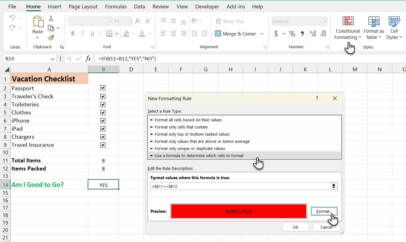
Apply Conditional Formatting
You can also color code the cell based on whether the values in cells B10 and B11 are equal. This is called Conditional Formatting.
Let’s see how to turn the cell red if not all the checkboxes are checked and green if they are. See our article about Conditional Formatting for information on how to create rules.
Select the cell next to «Am I good to go?». It’s B14 in this example spreadsheet.
Create a rule for this cell with the Conditional Formatting Rules Manager dialog box. Go to Home > Conditional Formatting > New Rules. Then, select the Use a formula to determine which cells to format rule.
Enter the following text in the Format values where this formula is true box.
Replace B11 and B12 with the cell references for your Total Items and Items Packed (or whatever you named these cells) values if they’re not the same. (See our guide to the Excel name box if you need more info on that.)
=$B11<>$B12
Then, click Format and select a red Fill color and click OK.
Create another new rule of the same type, but enter the following text in the Format values where this formula is true box. Again, replace the cell references to match your checklist.
=$B11=$B12
Then, click Format and select a green Fill color and click OK.
On the Conditional Formatting Rules Manager dialog box, enter an absolute reference for the cell you want to color green or red in the Applies to box.
Enter the same cell reference for both rules. In our example, we entered =$B$13.
Click OK.
The Am I good to go? cell in the B column turns green and reads YES when all the checkboxes are checked. If you uncheck any item, it will turn red and read NO.
Excel Checklist Complete? Check!
You can create a checklist in Excel easily enough. But it is just one type of list. You can also make dropdown lists in Excel with your custom items.
Do you also have information that you often use, like department names and people’s names? Try this method to create custom Excel lists for recurring data you always need.

If you’re building a spreadsheet to share with others or simply one for your own tracking, using a checklist can make data entry a breeze in Microsoft Excel. Here’s how to create a checklist in your spreadsheet and make it look like your own.
Why a checklist? You might use a checklist for tracking items to pack for a trip, products for your company, a holiday gift list, monthly bills, or keeping track of tasks. With a simple check box form control, you can create a checklist for anything you like in Excel.
Access the Developer Tab
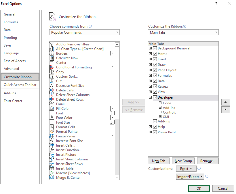
Before you can use the check box form control in Microsoft Excel, you need to make sure that you have access to the Developer tab. If you don’t see this tab at the top of Excel, it takes only a minute to add it.
Right-click anywhere on your Excel ribbon and select “Customize the Ribbon” from the drop-down list. Alternatively, you can click File > Options > Customize Ribbon from the menu.

On the right side of the window, under “Customize the Ribbon,” make sure “Main Tabs” is selected. Then in the list below it, check the box next to the “Developer” option.
Click “OK” and then close the Excel Options window.
RELATED: How to Add the Developer Tab to the Microsoft Office Ribbon
Add Your List of Items in Excel
The best way to begin your checklist is to add the list items. Even though you can always add or remove items later, this gives you the start you need to add your checkboxes. And you can, of course, add any row or column headers that you need.
Add Check Boxes for Your List Items
The action part of a checklist is the checkbox. And this is where the Developer tab comes into the mix, so be sure to select that tab. Go to an item on your list and click the cell next to it where you want a checkbox.
In the “”Controls” section of the ribbon, click the “Insert” button. Pick the “Checkbox” option in the “Form Controls” area.
You’ll then see your cursor change to crosshairs (like a plus sign). Drag a corner, and when you see your checkbox display, release.
By default, the checkbox will have a label attached to it which you will not need for a basic checklist. Select that text and hit your “Backspace” or “Delete” key. You can then select the checkbox control and drag a corner to resize it if needed.
Format Your Checkboxes
Once you insert a checkbox, you can make changes to its appearance if you like. Right-click the checkbox control. Make sure that you right-click the actual control and not the cell containing it. Select “Format Control” in the shortcut menu.
You’ll see tabs for “Colors and Lines” and “Size,” which give you easy ways to color the lines, add a fill color, scale the checkbox, and lock the aspect ratio. Be sure to click “OK” after making your changes.
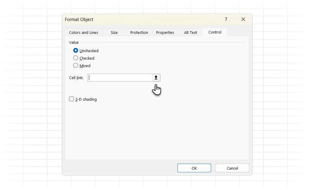
Checkbox Values and Cell Links
The other tab you may want to work with is the “Control” tab. This one lets you set the value, add a cell link if necessary, and apply 3D shading.
Checkbox Values
By default, a checkbox is unchecked when you insert it. Depending on the type of checklist you create, you might want the boxes checked by default instead. This forces the user to uncheck items they don’t want. To do this, mark “Checked” under “Value” in the Control tab and click “OK.”
Cell Links
If you plan to use your checklist in conjunction with Microsoft Excel formulas, you’ll likely use “Cell Link” on the “Control” tab. When you enter a cell into this box, it will display a True or False value based on the box being checked or unchecked.
Here’s an example. Say your checklist has 25 items and you plan to use the COUNTIF function to see how many of the items are checked. You can base your formula off of the True and False values associated with the checked and unchecked boxes.
RELATED: How to Use the COUNTIF Formula in Microsoft Excel
To use the “Cell Link,” simply type the cell reference into the box or click the cell in your spreadsheet to populate it automatically.
Add the Remaining Checkboxes
Follow the above steps to add checkboxes to your remaining list items. Or for a quicker way, use AutoFill to copy the checkboxes through the cells of your other items.
To use AutoFill, put your cursor on the bottom-right corner of the cell containing the checkbox. When you see the Fill Handle (plus sign), drag to fill the additional cells and release.
For marking off a list of to-dos, making a gift list and checking it twice, or tracking bills you pay each month, creating a checklist in Excel is a great way to go!
And if you like the list idea, how about adding a drop-down list in Microsoft Excel too?
READ NEXT
- › How to Insert a Checkbox in Microsoft Excel
- › How to Insert a Check Mark in Microsoft Excel
- › How to Count Checkboxes in Microsoft Excel
- › How to Create a Custom List in Microsoft Excel
- › How to Create a Basic Form in Microsoft Excel
- › How to Add a Checkbox in Google Sheets
- › How to Use Microsoft Excel Templates for Event Planning
- › HoloLens Now Has Windows 11 and Incredible 3D Ink Features

Add another medium to your ever-expanding checklist repertoire
We’ve already shown you how to create a Google Sheets checklist, and now, why not add an additional program to your checklist repertoire and learn how to create a Microsoft Excel checklist?

Checklists are a great tool for optimizing efficiency and improving productivity. They are especially great for ensuring you don’t forget an important task or valuable item. All you essentially need to create a checklist is a piece of paper and a pen. But knowing how to create one using other mediums can be a pretty cool skill to have.
Creating a checklist through Microsoft Excel requires utilizing the Checkbox control. Checkboxes are usually used when making forms, however, in this instance, they can also be used to create a checklist.
5 Steps for Creating a Microsoft Excel Checklist
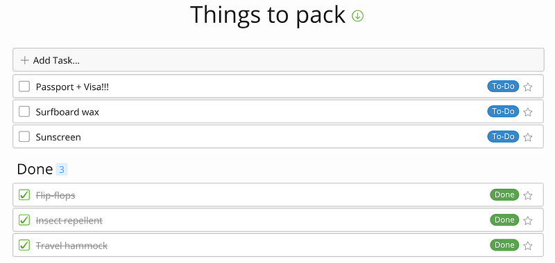
By using the example of creating a ‘things to pack for a holiday’ checklist, we’ll show you how it’s done on Microsoft Excel.
Step 1: Turn on the Developer tab
Enabling the Developer tab is the first thing you must do when creating an Excel checklist. To do this, go to File and select Options, then under the ‘Excel options’ dialogue box, click ‘Customize Ribbon’, as well as ensure you check the box beside ‘Developer’ on the right side by clicking ‘Ok’. You should be able to see the ‘Developer’ tab on the Excel ribbon.
Step 2: Set tasks in Excel
Under the ‘Things to pack’ column, start listing the items that you will need for your holiday.
Step 3: Input checkboxes
Right next to the ‘Things to pack’ column, we need to add Checkboxes. To do this, click on ‘Developer’, select ‘Insert’, and click the Checkbox icon under ‘Form Controls’. Then, click on the cell where the Checkbox will be placed. There may be some text that was added with the Checkbox. To remove this, simply right-click on the Checkbox, then ‘Edit Text’, and then delete the text.
Step 4: Appoint a cell to each Checkbox
In order for the values True and False to be shown when we tick and untick a Checkbox, a cell needs to be assigned to each Checkbox. Right-click on the Checkbox, then select ‘Formal Control’. Then, in the dialogue box under the ‘Control’ tab, input the address of the cell in the ‘Cell link’ box which you want to assign to the Checkbox.
Step 5: Don’t forget to apply conditional formatting!
And finally, for your Microsoft Excel checklist to be complete, ensure you apply conditional formatting. Select the tasks on your ‘Things to pack column’, then click on ‘Conditional Formatting’ found under the ‘Home’ tab, and click on ‘New Rule’. Select the rule type as ‘Use a formula to determine which cells to format’. In the condition textbox, you need to check the value of the cell which gets updated when the checkbox is ticked as True or False.
The next thing to do is to select the ‘Format’ button, then click ‘Strikethrough’ under ‘Effects’, select a red colour from the ‘Color’ dropdown, and press ‘Ok’. Repeat this for every task on your list. Make sure you hide the column that gets updated for every tick and untick a Checkbox so that your Excel spreadsheet only shows the item list and the checkboxes. Voila, your checklist is done!
Using Microsoft Excel to create a checklist does require a few steps to get right, but if you were after an electronic checklist that doesn’t require so much faffing about, there are software programs that allow you to do so in one simple click (literally!).
How to Create a Checklist with Zenkit
Zenkit is a project management tool that comes with many features designed to help improve the efficiency and productivity of you and your team. While a popular product to use professionally, it is also super handy to use when it comes to things within your personal life, like creating a checklist for things to pack for a holiday. Here’s how:
Create a new Collection and title it ‘Things to pack’. Once that’s done, start listing the items that you need. The recommended view is the ‘List view’, however, you do have the option of turning every view — except the Table view — into a checklist.
When checking items off your checklist, the item that has been marked as ‘checked’ will automatically move to the bottom of the list so that the unticked items have been prioritized to the top.
And, that’s pretty much it. The beauty of creating checklists with Zenkit is that it basically takes only one step to complete. You can turn any collection into a checklist by enabling the ‘Task List’ add-on. (Click here to see how.)
Final Thoughts
Whether created using Microsoft Excel, Zenkit, or just a pen and paper, there’s no doubt that checklists are the perfect tool to use in situations where it’s imperative to not forget an item or a task.
What do you use checklists for?
Cheers,
Dinnie and the Zenkit team
Was this article helpful? Please rate it!
There are many different apps to choose from if you want to create a checklist. But if you’re doing Excel work and have tasks associated with it, it may be easier to just include the checklist right within your spreadsheet. In this post, I’ll show you how you can make a checklist in Excel quickly and easily that you can re-use in many spreadsheets.
Step 1: Creating your list
Excel is an easy place to create a list since a spreadsheet is already in a grid format. You can use either numbers or letters as prefixes, or without anything at all:
Step 2: Add checkboxes
In order for this to look like a task list, we should add some checkboxes. If you don’t have the Developer tab enabled in Excel, make sure to do so. Under Excel Options, you’ll have an option to customize the Ribbon. This is where you can select which tabs you want to have enabled:
Once enabled, go to the Developer tab and click on the Insert button. Select the checkbox icon that is under the Form Controls section:
Then, use the mouse to drag and create a checkbox. It will automatically create some generic text to say ‘Check Box 1’ — you can remove this as it is unnecessary. Once you’ve got the checkbox in the position you want (and within its own cell), copy the entire cell and paste it over so that you have a checkbox next to each task:
Each checkbox can be linked to a specific cell. And every time you click the checkbox, the value of that cell will toggle between TRUE and FALSE, to indicate if the box is ticked or not. To create a link, right-click on a checkbox and select Format Control. Then, under the Control section, select a cell in the Cell Link section:
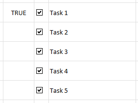
Then, when the checkbox is ticked or unticked, here’s how the values in the will appear in the linked cell:
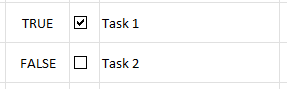
The danger with copying these checkboxes after you have linked a cell, is that those cell links won’t change; multiple checkboxes will be linked to the same cell:
To correct this, you will need to modify the cell link for each checkbox. Once that’s done, it’s time to move on to the last step.
Step 3: Add conditional formatting
Right now, ticking the checkbox doesn’t do anything but show a TRUE or FALSE value. In this step, I’m going to add some conditional formatting to also cross out the item. To do this, I’m going to highlight the column that has the tasks (column B) and create some conditional formatting rules:
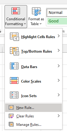
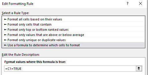
I’m going to create a rule that looks at the column that contains the cell link values (column C). It will check if the value is set to TRUE using the following formula:
=C1=TRUE
Then, under the Format options, I will apply a strikethrough effect:
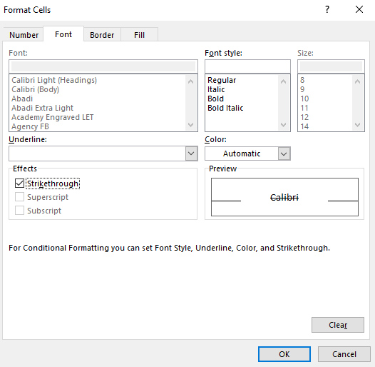
Now, when a checkbox is ticked, the text will have a strikethrough effect:
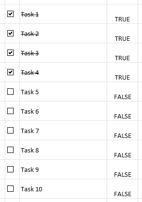
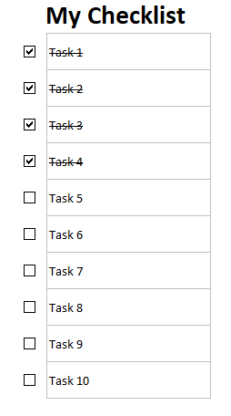
The TRUE/FALSE values can be hidden since they don’t need to be visible in order for the checkboxes and strikethrough effects to work. The only other changes you may want to make at this point relate to formatting. This includes applying a header. Here’s what your finished checklist might look like with some additional formatting:
If you liked this post on How to Make a Checklist in Excel, please give this site a like on Facebook and also be sure to check out some of the many templates that we have available for download. You can also follow us on Twitter and YouTube.