
Excel for Microsoft 365 Excel 2021 Excel 2019 Excel 2016 Excel 2013 Excel 2010 Excel 2007 More…Less
Important:
-
When you break a link to the source workbook of an external reference, all formulas that use the value in the source workbook are converted to their current values. For example, if you break the link to the external reference =SUM([Budget.xls]Annual!C10:C25), the SUM formula is replaced by the calculated value—whatever that may be. Also, because this action cannot be undone, you may want to save a version of the destination workbook as a backup.
-
If you use an external data range, a parameter in the query may be using data from another workbook. You may want to check for and remove any of these type of links.
Break a link
-
On the Data tab, in the Connections group, click Edit Links.

Note: The Edit Links command is unavailable if your file does not contain linked information.
-
In the Source list, click the link that you want to break.
-
To select multiple linked objects, hold down the CTRL key, and click each linked object.
-
To select all links, press Ctrl+A.
-
-
Click Break Link.

Delete the name of a defined link
If the link used a defined name, the name is not automatically removed. You may want to delete the name as well, by following these steps:
-
On the Formulas tab, in the Defined Names group, click Name Manager.
-
In the Name Manager dialog box, click the name that you want to change.
-
Click the name to select it.
-
Click Delete.
-
Click OK.
Need more help?
You can always ask an expert in the Excel Tech Community or get support in the Answers community.
Need more help?
Want more options?
Explore subscription benefits, browse training courses, learn how to secure your device, and more.
Communities help you ask and answer questions, give feedback, and hear from experts with rich knowledge.
September 09, 2018/
Chris Newman
How To Break External Links
So you’re on a mission to break/remove external links from your Excel workbook, huh? Seems like it should be easy, but as you are probably finding out, it sometimes isn’t as easy as clicking the «break links» button (unfortunately).
In this guide, I am going to walk you through all the hiding places where those pesky little external links may be lurking.
Guide Contents
-
Break External Links From Cells
-
Break External Links In Charts
-
Break External Links In Shapes
-
Break External Links In Named Ranges
-
Break External Links In Pivot Tables
-
Break External Links In Data Validation Rules
Removing External Links From Cells
External links in cells are typically the easiest to find and remove. You should always start by using the Edit Links Dialog. You can quickly break links to external Excel files by using the following steps:
-
Navigate to the Data Tab in the Excel Ribbon
-
Within the Queries & Connections button group, select the Edit Links Button
-
Select 1 or more Source Files from the Edit Link Dialog’s Listbox
-
Click Break Link
-
When you see a warning message that this action cannot be undone, click the Break Links button
When you see the Edit Links dialog appears, you will see a listing of all the external Excel files that are getting data pulled from them. To remove/break the link, simply select the rows you wish to remove and click the Break Link button.
You will get a prompt (shown below) asking if you are sure you want to break the links as this action is irreversible.
Click Break Links and all your links «should» be broken. In a perfect world, the Edit Links button will be grayed out and all your external links will be removed.
However, this is far from a perfect world! Sometimes certain links cannot be broken via the Edit Links dialog. In other cases, you will still get prompts stating that there are external links in your workbook.
If you are still thinking there are external links in your workbook, continue reading on to learn where else those pesky links may be hiding.
VBA Code Solution To Automate This
If you would like to automate this process with a VBA macro, you can check out a small macro I have put together to automatically remove links from your Excel Workbook.
Removing External Links From Charts
External Links can reside inside any textbox of a Chart object. This includes the:
-
Chart Title
-
Axis Labels
-
Data Labels
Click on each Chart object that could have a formula linked to it and look in the Excel Formula Bar to see if the reference is outside the workbook.
Removing External Links From Shapes
If you have shapes with formulas connected to them, there could be a possibility that the formulas have external links. You can easily check by clicking on the shape in question and looking at the contents of the Formula Bar.
If you have a lot of shapes to look through, take the following steps to quickly cycle through all the shapes:
-
Hit the F5 key to open the Go To dialog box
-
Click on Special
-
Only check Objects
-
Click OK.
You will now have all the shapes in the spreadsheet selected. To cycle through each shape, just hit the Tab key and keep your eye on the Formula Bar for any formulas that may appear.
Removing External Links From Named Ranges
Removing External Links From Pivot Tables
The Source Data for a Pivot Table can be linked to an outside file. Follow these steps to check your Pivot Table’s Source Data connection.
-
Select a cell within your Pivot Table
-
Navigate to the PivotTable Tools Analyze Tab
-
Click the Change Data Source button
-
Look inside the Change PivotTable Data Source dialog box and confirm your data is not linked externally
Removing External Links From Data Validation Rules
External Links can reside in Data Validation rules. This can occur as the Source input for a List rule. You can manually search through each of your Data Validation rules within your workbook however, that may be a daunting task if you have a lot of tabs to search through. An easier way is to use the Compatibility Checker to search for you.
Using The Compatibility Checker to Find Data Validation Errors:
-
Select the File tab
-
In the Info section, select the Check for Issues drop-down
-
Select Check Compatibility
-
In the Compatibility Checker dialog box click the Copy to New Sheet button
-
You should see a new sheet with all the issues listed. Use the keyboard shortcut ctrl + F to bring up the Find dialog and search for instances of «data validation»
-
If you have any external links or errors in your data validation rules, you’ll find sections on the sheet with hyperlinks taking you to the cells with the data validation that was flagged
-
Click on each hyperlink and check the data validation rule while the cell range is still selected
-
If you see any external references in the Source field, you’ll most likely want to hit the Clear All button to get rid of the external link
Any Other Areas?
Have you found any other areas in your spreadsheets where External Links were hiding? Let me know in the comments and I’ll keep this article updated so we have a nice comprehensive list!

About The Author
Hey there! I’m Chris and I run TheSpreadsheetGuru website in my spare time. By day, I’m actually a finance professional who relies on Microsoft Excel quite heavily in the corporate world. I love taking the things I learn in the “real world” and sharing them with everyone here on this site so that you too can become a spreadsheet guru at your company.
Through my years in the corporate world, I’ve been able to pick up on opportunities to make working with Excel better and have built a variety of Excel add-ins, from inserting tickmark symbols to automating copy/pasting from Excel to PowerPoint. If you’d like to keep up to date with the latest Excel news and directly get emailed the most meaningful Excel tips I’ve learned over the years, you can sign up for my free newsletters. I hope I was able to provide you with some value today and I hope to see you back here soon!
— Chris
Founder, TheSpreadsheetGuru.com
If in our data any cells have values starting with https:// or www. it is considered a hyperlink. When we click on the cells, we are redirected to our browser regardless of whether the page exists. The method to remove hyperlinks in Excel is to select the cell or the column containing hyperlinks, right-click on it, and select the “Remove Hyperlinks” option.
Let us understand how to remove hyperlinks in Excel with examples.
You can download this Remove Hyperlinks in Excel Template here – Remove Hyperlinks in Excel Template
Hyperlinks are very powerful. It can take you to the desired location and shorten our time. However, if you already know how to insert hyperlinksTo insert a hyperlink, right-click on the cell, click on hyperlink, and then choose the last option, which will open a wizard box to insert a hyperlink. Then, in the field for an address, type the hyperlink’s URL.read more, you must also know how to remove them.
We are telling this because Excel automatically creates a hyperlink when entering an email ID and URL. It will be very irritating to work with because every time you click on them, it will take you to their window and make you angry. (We get angry whenever it takes me to an outlook or web browser).
In these cases, we need to remove unwanted Excel hyperlinks automatically created by Excel when we insert an email ID or URL.
Table of contents
- How to Remove Hyperlinks in Excel?
- Method #1 – Remove Excel Hyperlink in Just a click
- Alternative Method to Remove Hyperlinks in Excel
- Method #2 – Remove Hyperlink in Excel Using Find and Replace
- Method #3 – Remove Hyperlink in Excel Using VBA Code
- Restrict Excel from Creating Hyperlinks
- Things to Remember
- Recommended Articles
- Method #1 – Remove Excel Hyperlink in Just a click
Method #1 – Remove Excel Hyperlink in Just a click
In this example, we are using three different types of hyperlinks. In column A, we have worksheet hyperlinks we have created. In the second column, we have the email IDs, and Excel itself creates hyperlinks. Finally, have the website address in the third column, and Excel creates hyperlinks.
Below are the steps used to remove Excel hyperlinks in just a click:
- First, select the “Email ID” column.

- Right-click and select the “Remove Hyperlinks” option.

- It will instantly remove the hyperlinks in Excel and formatting.


Alternative Method to Remove Hyperlinks in Excel
There is an alternative method to remove the hyperlink in Excel.
Step 1: Select the targeted data first.

Step 2: Then, on the “Home” tab, find the “Clear “button in the “Editing” group and click on the dropdown list.

Step 3: This can also remove the hyperlink in Excel.

Method #2 – Remove Hyperlink in Excel Using Find and Replace
We can also remove hyperlinks using “Find and Replace ExcelFind and Replace is an Excel feature that allows you to search for any text, numerical symbol, or special character not just in the current sheet but in the entire workbook. Ctrl+F is the shortcut for find, and Ctrl+H is the shortcut for find and replace.read more“. Follow the below steps.
Step 1: Press “Ctrl + F.”

Step 2: Click on “Options.”

Step 3: Now click on “Format” and select “Choose Format from Cell.”

Step 4: Now, select the hyperlinked cell, showing the preview in blue.

Step 5: Click on “Find All.” It will display all the hyperlinked cells.

Step 6: Now, select those using the “Shift + Down Arrow” key.

Step 7: Exit from the “Find & Replace” window.
Step 8: Now, all the hyperlinked cells are selected. Right-click and click on “Remove Hyperlinks.”
Method #3 – Remove Hyperlink in Excel Using VBA Code
VBA code is the one-time code that we can regularly use whenever we want. VBA codeVBA code refers to a set of instructions written by the user in the Visual Basic Applications programming language on a Visual Basic Editor (VBE) to perform a specific task.read more instantly removes the hyperlink from the active sheet and the entire workbook.
Follow the below steps to start using it.
Step 1: Press the “Alt + F11” key to open the VBA editorThe Visual Basic for Applications Editor is a scripting interface. These scripts are primarily responsible for the creation and execution of macros in Microsoft software.read more window in the current worksheet.

Step 2: Click on the “Insert” and insert “Module.”

Step 3: Copy and paste the below code into the newly inserted module and click on “F5” to run the code.
The below code is to Remove hyperlinks from One Sheet at a time.
Sub Remove_Hyperlinks()
‘One sheet at a time
ActiveSheet.Hyperlinks.Delete
End Sub

The below code is to Remove from the entire workbook.
Sub Remove_Hyperlinks1()
Dim Ws As Worksheet
For Each Ws In ActiveWorkbook.Worksheets
ActiveSheet.Hyperlinks.Delete
Next Ws
End Sub

The first code will remove the hyperlink in the active sheet only. The second code will discard the hyperlink in the whole Excel workbook.
Run this code using the F5 key.
Note: Do not forget to save the workbook as a Macro-Enabled Workbook.
Excel automatically creates hyperlinks for email ID and URL.
Unfortunately, it is one of the irritating things to work with.
However, we can disable the hyperlink’s auto-creation option by changing the settings.
Restrict Excel from Creating Hyperlinks
Excel creates auto hyperlinks because there is a default setting to it. Email ID extensions and WWW web addresses are automatically converted to hyperlinks.
Follow the below steps to restrict Excel from creating auto hyperlinks.
Step 1: Click on the “File” option.

Step 2: Now, click on “Options.”

Step 3: Click on “Proofing” and “Autocorrect Options.”
Step 4: Now, select “AutoFormatThe AutoFormat option in Excel is a unique way of formatting data quickly.read more As You Type”.

Step 5: Uncheck the box: Internet and network paths with hyperlinks.

Step 6: Click on “OK” and close this box.
Now, try adding a few email IDs and URL addresses.
Excel stops creating auto hyperlinks for emails and URLs.
Things to Remember
- Excel auto hyperlinks for email and URL.
- We must use a “Clear” hyperlink option to remove hyperlinks in Excel and retain formatting.
- Changes the default settings to restrict Excel not to creating auto hyperlinks.
- We can remove hyperlinks from the entire workbook by using the VBA code.
Recommended Articles
This article is a guide on how to remove Hyperlinks in Excel. Here, we discuss the three useful methods to remove hyperlinks in Excel, along with Excel examples and downloadable Excel templates. You may also look at these useful functions in Excel: –
- VBA HyperlinksHyperlinks are URLs attached to a value that appear when we hover the mouse over it. When we click on it, the URL is opened. In VBA, we have an inbuilt property to create hyperlinks. We use the add method and the hyperlink statement to insert a hyperlink.read more
- Text to Columns in Excel
- Checkbox in Excel
- How to Show Excel Formula?
Note: This tutorial on how to remove hyperlinks in Excel is suitable for all Excel versions including Office 365.
The hyperlink is no doubt a very useful feature. It enables us to easily redirect to other resources simply by clicking on them. These resources can range from web pages, local documents, or other online content.

But, unnecessary usage of hyperlinks can be very irritating. It will create a lot of clutter and confusion if overused.
Unfortunately, Excel automatically converts all URLs or e-mail addresses into clickable hyperlinks by default. This can become very frustrating in the long run, especially if you need to keep your data clean and organised.
In this guide, I’ll teach you how to remove hyperlinks in Excel like a pro and help you save precious time.
Table Of Contents
- Disable Automatic Hyperlink in Excel
- How to Remove Hyperlinks in Excel in One Go?
- How to Remove Hyperlinks in Excel Using VBA Code
- FAQs
- How do I remove hyperlinks in Excel without losing formatting?
- How to remove multiple hyperlinks in excel?
- Let’s Wrap Up
You can download the free sample Excel Sheet here and follow along with this guide.

Related:
How to Use the Format Painter Excel Feature? — 3 Bonus Tips
How to Indent in Excel? 3 Easy Methods
How to Add Subscript in Excel? (6 Best Methods)
Disable Automatic Hyperlink in Excel
Prevention is always better than cure. First, I’ll show you how to avoid this hyperlink mess in the first place. Please follow these steps:
- Go to the File tab and click on Options. This will open the Excel Options window. You can also use the keyboard shortcuts Alt+T+O or Alt+F+T to directly open the Excel options window.
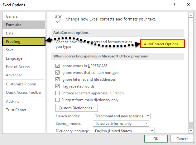
- Under Excel Options, open the Proofing tab and click on the AutoCorrect Options button inside it.

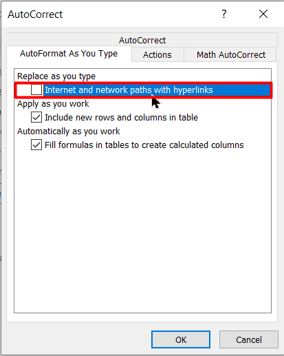
- In the AutoCorrect Options window, deselect the Internet and network paths with hyperlinks option under the AutoFormat as you type tab.
- Click OK to save your changes and exit the window.
As soon as you do this, Excel will no longer convert URLs or internet addresses to hyperlinks.
In case you need to add hyperlinks, select the text or object and press Ctrl+K to add them.
Also Read:
How to Apply the Accounting Number Format in Excel? (3 Best methods)
How to Enable Excel Dark Mode? 3 Simple Steps
The FORMULATEXT Excel Function – 2 Best Examples
How to Remove Hyperlinks in Excel in One Go?
If you are using any version later than Excel 2010, you can easily remove multiple or all hyperlinks in one go.
All you need to do is select the range of cells that contain the hyperlinks. You can select the entire sheet using Ctrl+A or even multiple worksheets at a time.
Then, right-click anywhere inside the selected cells and choose the Remove Hyperlinks option from the Context menu. You can access this menu by using the shortcut Shift+F10.

Or click on the Clear option under the Editing group of the Home tab. In the drop-down menu choose Remove Hyperlinks.

This will remove all the hyperlinks in your selection in one go.
How to Remove Hyperlinks in Excel Using VBA Code
Let us say, you are using an older version of Excel. Or you are simply tired of using the right-click context menu, as there may be too many hyperlinks in your workbook.
How to remove hyperlink in Excel with a single button click?
Fortunately, VBA codes come to our rescue.
Hit Alt+F11 to open your VBA editor.
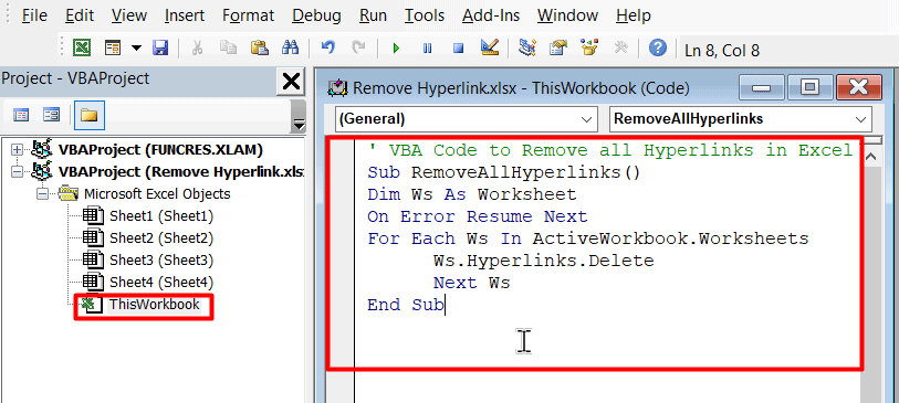
Now, in the Project Window displayed on the left-hand side of the VBA editor, double-click on ThisWorkbook.
Next, in the Module window copy and paste the following VBA code:
' VBA Code to Remove all Hyperlinks in Excel
Sub RemoveAllHyperlinks()
Dim Ws As Worksheet
On Error Resume Next
For Each Ws In ActiveWorkbook.Worksheets
      Ws.Hyperlinks.Delete
      Next Ws
End Sub
Then, hit F5 to run the VBA code module.
This will remove all the hyperlinks in your workbook in one go. You no longer need to worry about them. But, keep in mind that this action is irreversible. You cannot undo the removal of hyperlinks using Ctrl+Z.
Let me share an interesting tip with you.
You can actually save this VBA code as an easy-to-use, click and forget button on your Quick Access toolbar. Just follow these instructions:
- Once you have added the VBA code module, close the VBA editor window.
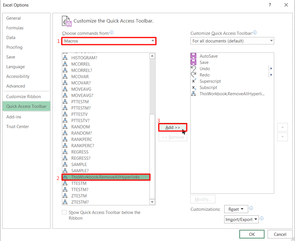
- Click on the Customize Quick Access Toolbar button and choose More Commands

- In the Excel Options window, under the Choose commands from the drop-down list, select Macros.
- Now scroll down and select the VBA code module that we just added.
- Click on Add and click OK.
That’s all. A quick-access button for running this VBA code will be added to the Quick Access toolbar.
You can save your Worksheet as a macro-enabled workbook and keep using this ready-made button for quickly removing all hyperlinks.

Suggested Reads:
How to Autofit Excel Cells? 3 Best Methods
How to Extract an Excel Substring? – 6 Best Methods
How to Shade Every Other Row in Excel? (5 Best Methods)
FAQs
How do I remove hyperlinks in Excel without losing formatting?

To clear hyperlinks without changing format settings, first select the cell or range of cells that contain the hyperlinks. Then, click on the Clear option in the Editing group of the Home Tab.
Now, select the Clear Hyperlinks option under the drop-down list. This will display a small pink-colour eraser at the right bottom of your selection. Click on it and choose Clear Hyperlinks Only to clear hyperlinks but keep the formatting.
How to remove multiple hyperlinks in excel?
If you have multiple hyperlinks spread over multiple sheets, the best way to clear them all is to run the following VBA code in the VBA editor.
‘ VBA Code to Remove all Hyperlinks in Excel
Sub RemoveAllHyperlinks()
Dim Ws As Worksheet
On Error Resume Next
For Each Ws In ActiveWorkbook.Worksheets
Ws.Hyperlinks.Delete
Next Ws
End Sub
Let’s Wrap Up
In this guide, we saw how to remove hyperlinks in Excel the easy way. I also talked about how to avoid them in the first place. I hope this will make your work less stressful and more fun.
If you have any questions about this or any other Excel feature, please feel free to ask in the comments section.
Need more high-quality Excel guides? Check out our free Excel resources centre.
Simon Sez IT has been teaching Excel for over ten years. For a low, monthly fee you can get access to 100+ IT training courses by seasoned professionals. Click here for advanced Excel courses with in-depth training modules.
Adam Lacey

Adam Lacey is an Excel enthusiast and online learning expert. He combines these two passions at Simon Sez IT where he wears a number of different hats.When Adam isn’t fretting about site traffic or Pivot Tables, you’ll find him on the tennis court or in the kitchen cooking up a storm.
Содержание
- Добавление гиперссылок
- Способ 1: вставка безанкорных гиперссылок
- Способ 2: связь с файлом или веб-страницей через контекстное меню
- Способ 3: связь с местом в документе
- Способ 4: гиперссылка на новый документ
- Способ 5: связь с электронной почтой
- Способ 6: вставка гиперссылки через кнопку на ленте
- Способ 7: функция ГИПЕРССЫЛКА
- Удаление гиперссылок
- Способ 1: удаление с помощью контекстного меню
- Способ 2: удаление функции ГИПЕРССЫЛКА
- Способ 3: массовое удаление гиперссылок (версия Excel 2010 и выше)
- Способ 4: массовое удаление гиперссылок (версии ранее Excel 2010)
- Вопросы и ответы

С помощью гиперссылок в Экселе можно ссылаться на другие ячейки, таблицы, листы, книги Excel, файлы других приложений (изображения и т.п.), различные объекты, веб-ресурсы и т.д. Они служат для быстрого перехода к указанному объекту при клике по ячейке, в которую они вставлены. Безусловно, в сложно структурированном документе использование этого инструмента только приветствуется. Поэтому пользователю, который хочет хорошо научиться работать в Экселе, просто необходимо освоить навык создания и удаления гиперссылок.
Интересно: Создание гиперссылок в Microsoft Word
Добавление гиперссылок
Прежде всего, рассмотрим способы добавления гиперссылок в документ.
Способ 1: вставка безанкорных гиперссылок
Проще всего вставить безанкорную ссылку на веб-страницу или адрес электронной почты. Безанкорная гиперссылка – эта такая ссылка, адрес которой прямо прописывается в ячейке и виден на листе без дополнительных манипуляций. Особенностью программы Excel является то, что любая безанкорная ссылка, вписанная в ячейку, превращается в гиперссылку.
Вписываем ссылку в любую область листа.
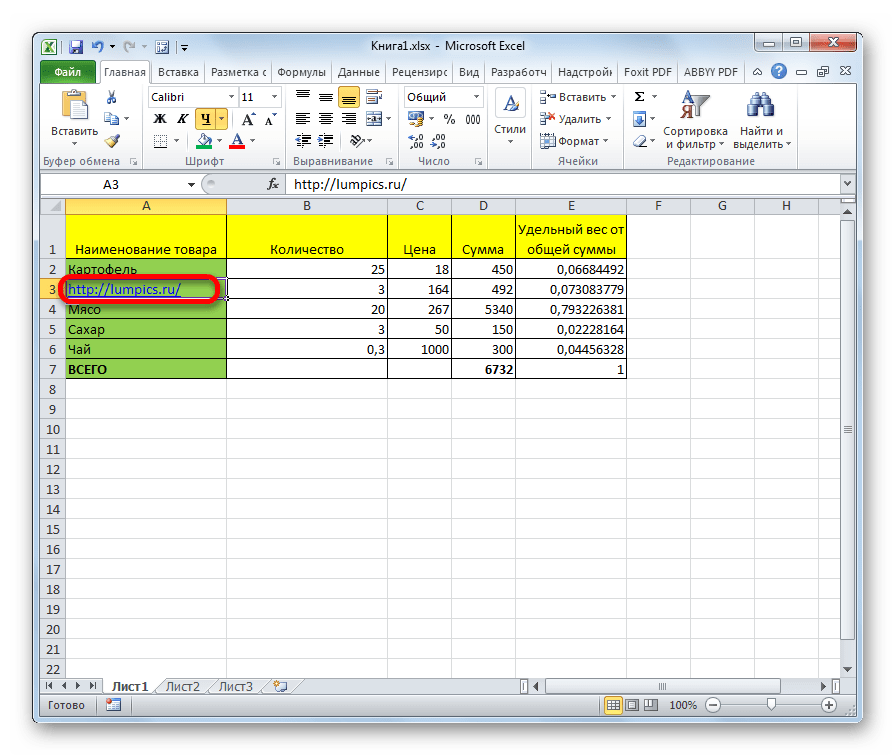
Теперь при клике на данную ячейку запустится браузер, который установлен по умолчанию, и перейдет по указанному адресу.
Аналогичным образом можно поставить ссылку на адрес электронной почты, и она тут же станет активной.

Способ 2: связь с файлом или веб-страницей через контекстное меню
Самый популярный способ добавления ссылок на лист – это использование контекстного меню.
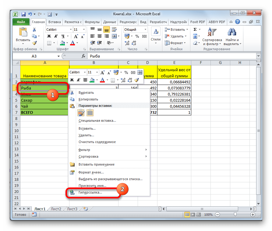
- Выделяем ячейку, в которую собираемся вставить связь. Кликаем правой кнопкой мыши по ней. Открывается контекстное меню. В нём выбираем пункт «Гиперссылка…».
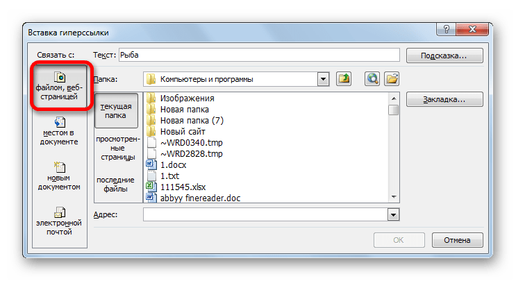
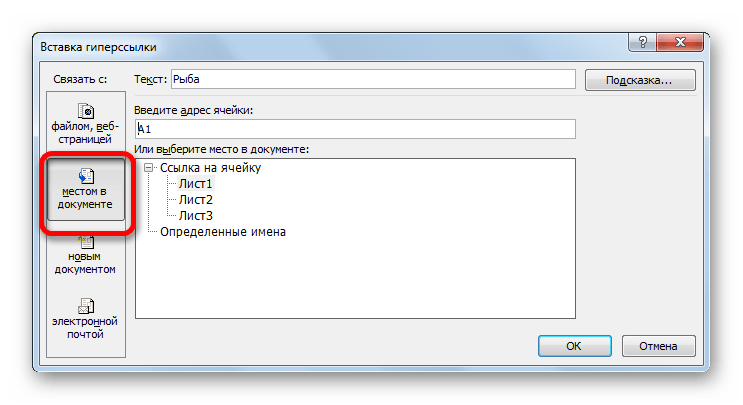
- Сразу после этого открывается окно вставки. В левой стороне окна расположены кнопки, нажав на одну из которых пользователь должен указать, с объектом какого типа хочет связать ячейку:
- с внешним файлом или веб-страницей;
- с местом в документе;
- с новым документом;
- с электронной почтой.
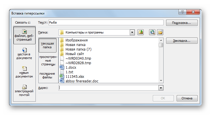
Так как мы хотим показать в этом способе добавления гиперссылки связь с файлом или веб-страницей, то выбираем первый пункт. Собственно, его и выбирать не нужно, так как он отображается по умолчанию.
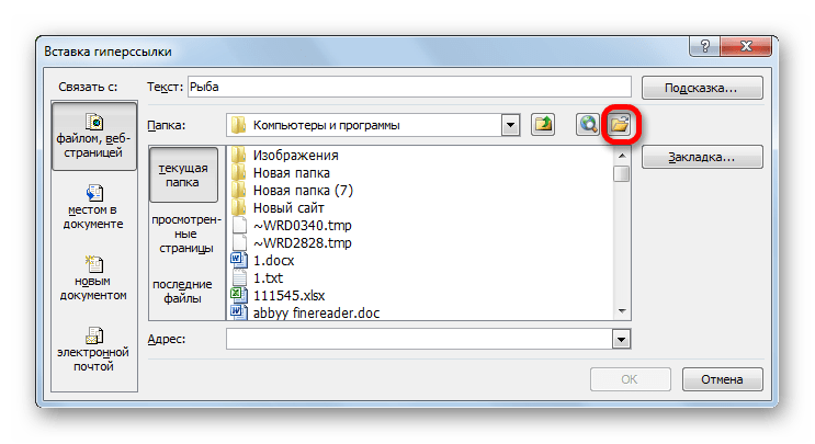
- В центральной части окна находится область Проводника для выбора файла. По умолчанию Проводник открыт в той же директории, где располагается текущая книга Excel. Если нужный объект находится в другой папке, то следует нажать на кнопку «Поиск файла», расположенную чуть выше области обозрения.
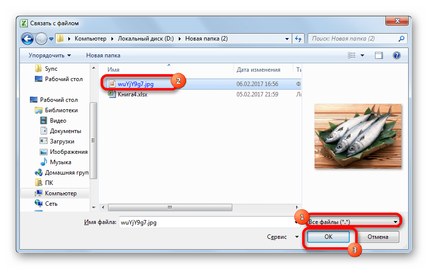
- После этого открывается стандартное окно выбора файла. Переходим в нужную нам директорию, находим файл, с которым хотим связать ячейку, выделяем его и жмем на кнопку «OK».

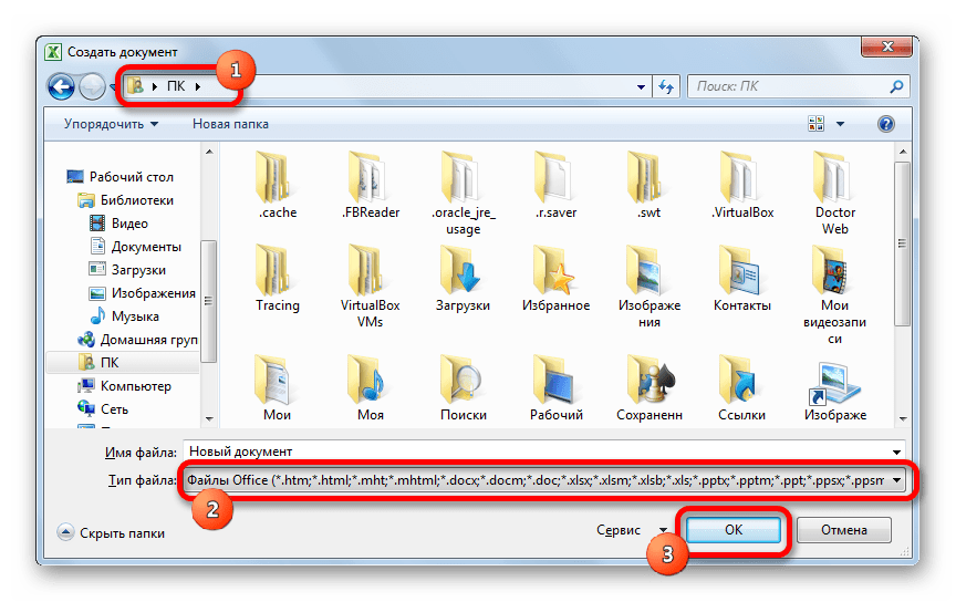
Внимание! Для того, чтобы иметь возможность связать ячейку с файлом с любым расширением в окне поиска, нужно переставить переключатель типов файлов в положение «Все файлы».
- После этого координаты указанного файла попадают в поле «Адрес» окна вставки гиперссылки. Просто жмем на кнопку «OK».

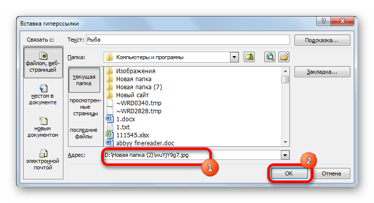
Теперь гиперссылка добавлена и при клике на соответствующую ячейку откроется указанный файл в программе, установленной для его просмотра по умолчанию.
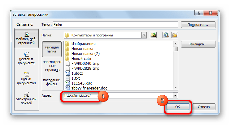
Если вы хотите вставить ссылку на веб-ресурс, то в поле «Адрес» нужно вручную вписать url или скопировать его туда. Затем следует нажать на кнопку «OK».
Способ 3: связь с местом в документе
Кроме того, существует возможность связать гиперссылкой ячейку с любым местом в текущем документе.
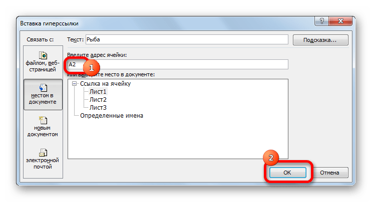
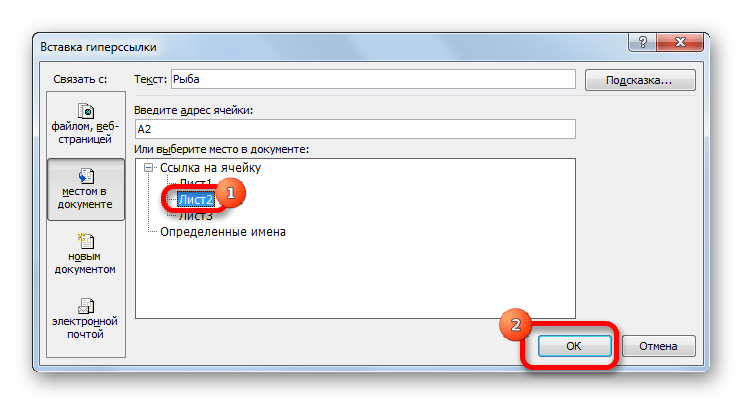
- После того, как выделена нужная ячейка и вызвано через контекстное меню окно вставки гиперссылки, переключаем кнопку в левой части окна в позицию «Связать с местом в документе».
- В поле «Введите адрес ячейки» нужно указать координаты ячейки, на которые планируется ссылаться.

Вместо этого в нижнем поле можно также выбрать лист данного документа, куда будет совершаться переход при клике на ячейку. После того, как выбор сделан, следует нажать на кнопку «OK».
Теперь ячейка будет связана с конкретным местом текущей книги.
Способ 4: гиперссылка на новый документ
Ещё одним вариантом является гиперссылка на новый документ.
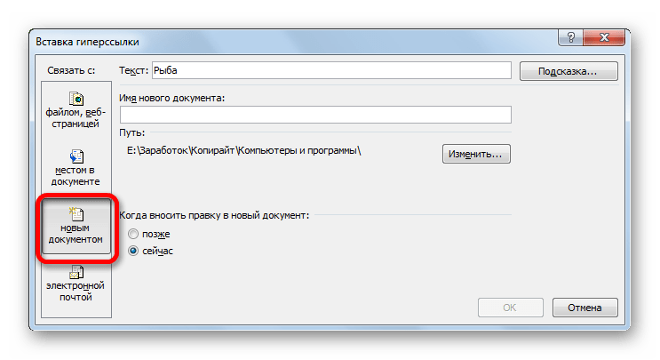
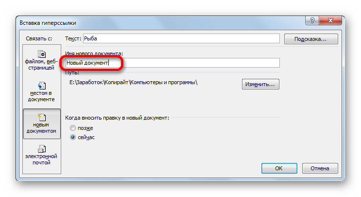
- В окне «Вставка гиперссылки» выбираем пункт «Связать с новым документом».
- В центральной части окна в поле «Имя нового документа» следует указать, как будет называться создаваемая книга.
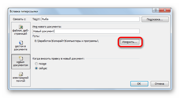
- По умолчанию этот файл будет размещаться в той же директории, что и текущая книга. Если вы хотите сменить место расположения, нужно нажать на кнопку «Изменить…».
- После этого, открывается стандартное окно создания документа. Вам нужно будет выбрать папку его размещения и формат. После этого нажмите на кнопку «OK».
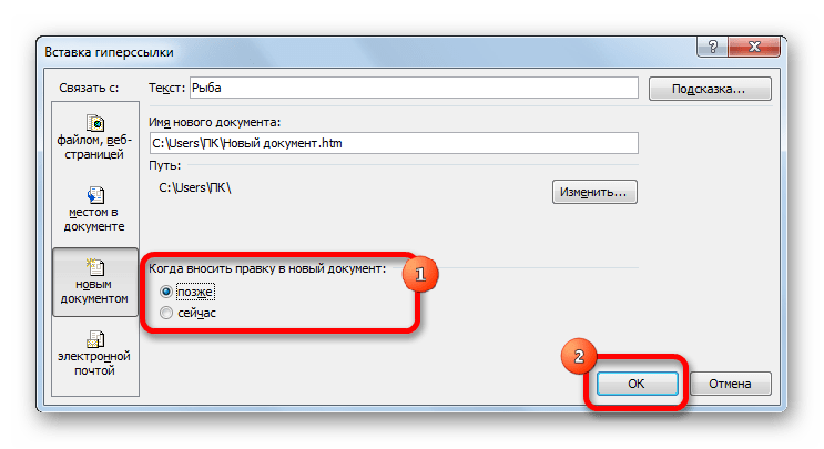
- В блоке настроек «Когда вносить правку в новый документ» вы можете установить один из следующих параметров: прямо сейчас открыть документ для изменения, или вначале создать сам документ и ссылку, а уже потом, после закрытия текущего файла, отредактировать его. После того, как все настройки внесены, жмем кнопку «OK».
После выполнения этого действия, ячейка на текущем листе будет связана гиперссылкой с новым файлом.
Способ 5: связь с электронной почтой
Ячейку при помощи ссылки можно связать даже с электронной почтой.
- В окне «Вставка гиперссылки» кликаем по кнопке «Связать с электронной почтой».
- В поле «Адрес электронной почты» вписываем e-mail, с которым хотим связать ячейку. В поле «Тема» можно написать тему письма. После того, как настройки выполнены, жмем на кнопку «OK».

Теперь ячейка будет связана с адресом электронной почты. При клике по ней запуститься почтовый клиент, установленный по умолчанию. В его окне уже будет заполнен предварительно указанный в ссылке e-mail и тема сообщения.
Способ 6: вставка гиперссылки через кнопку на ленте
Гиперссылку также можно вставить через специальную кнопку на ленте.
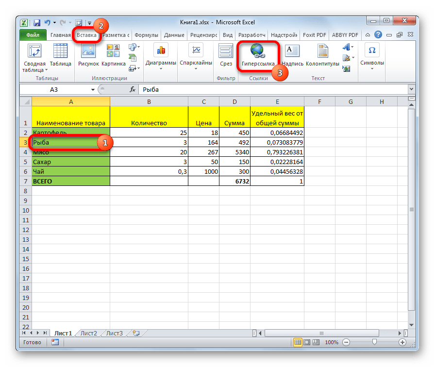
- Переходим во вкладку «Вставка». Жмем на кнопку «Гиперссылка», расположенную на ленте в блоке инструментов «Ссылки».
- После этого, запускается окно «Вставка гиперссылки». Все дальнейшие действия точно такие же, как и при вставке через контекстное меню. Они зависят от того, какого типа ссылку вы хотите применить.
Способ 7: функция ГИПЕРССЫЛКА
Кроме того, гиперссылку можно создать с помощью специальной функции.
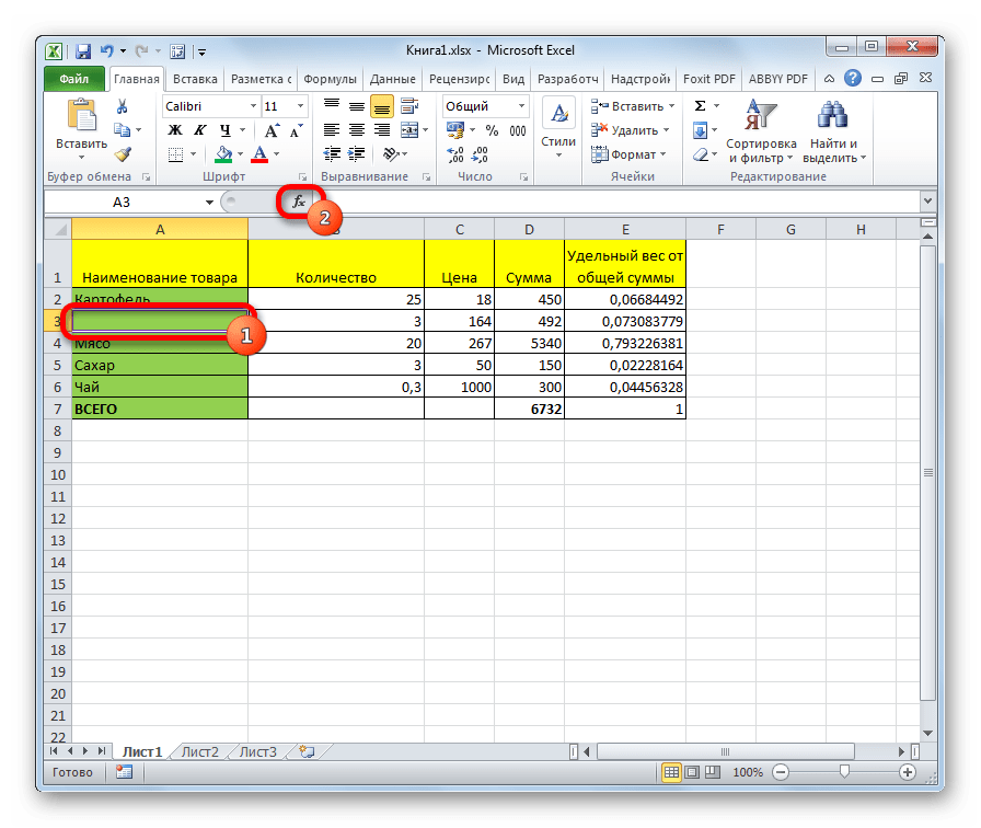
- Выделяем ячейку, в которую будет вставлена ссылка. Кликаем на кнопку «Вставить функцию».
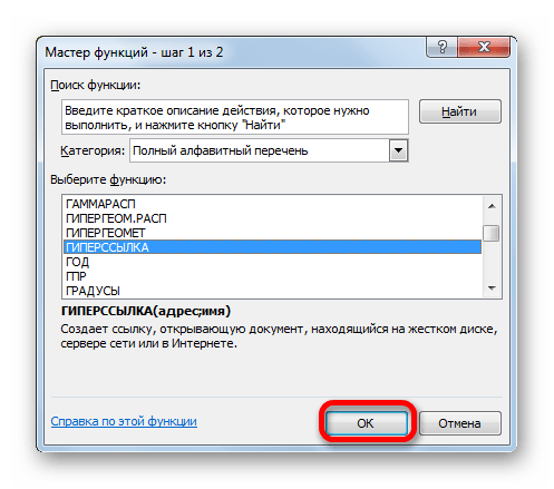
- В открывшемся окне Мастера функций ищем наименование «ГИПЕРССЫЛКА». После того, как запись найдена, выделяем её и жмем на кнопку «OK».
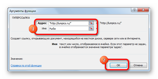
- Открывается окно аргументов функции. ГИПЕРССЫЛКА имеет два аргумента: адрес и имя. Первый из них является обязательным, а второй необязательным. В поле «Адрес» указывается адрес сайта, электронной почты или место расположения файла на жестком диске, с которым вы хотите связать ячейку. В поле «Имя», при желании, можно написать любое слово, которое будет видимым в ячейке, тем самым являясь анкором. Если оставить данное поле пустым, то в ячейке будет отображаться просто ссылка. После того, как настройки произведены, жмем на кнопку «OK».
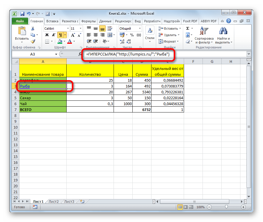
После этих действий, ячейка будет связана с объектом или сайтом, который указан в ссылке.
Урок: Мастер функций в Excel
Удаление гиперссылок
Не менее важен вопрос, как убрать гиперссылки, ведь они могут устареть или по другим причинам понадобится изменить структуру документа.
Интересно: Как удалить гиперссылки в Майкрософт Ворд
Способ 1: удаление с помощью контекстного меню
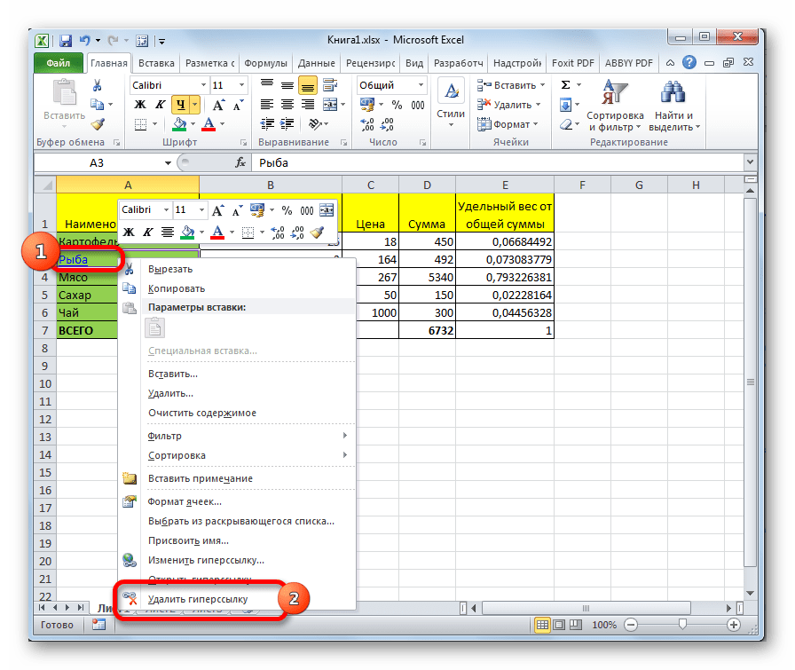
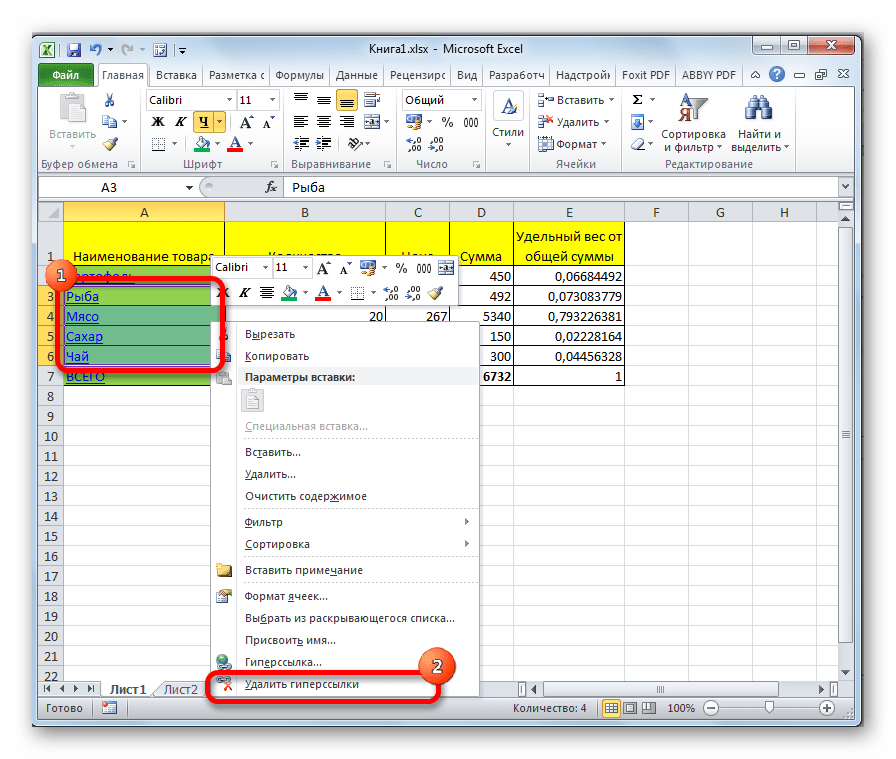
Самым простым способом удаления ссылки является использования контекстного меню. Для этого просто кликаем по ячейке, в которой расположена ссылка, правой кнопкой мыши. В контекстном меню выбираем пункт «Удалить гиперссылку». После этого она будет удалена.
Способ 2: удаление функции ГИПЕРССЫЛКА
Если у вас установлена ссылка в ячейке с помощью специальной функции ГИПЕРССЫЛКА, то удалить её вышеуказанным способом не получится. Для удаления нужно выделить ячейку и нажать на кнопку Delete на клавиатуре.

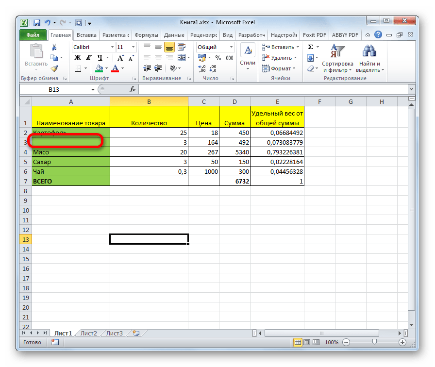
При этом будет убрана не только сама ссылка, но и текст, так как в данной функции они полностью связаны.
Способ 3: массовое удаление гиперссылок (версия Excel 2010 и выше)
Но что делать, если в документе очень много гиперссылок, ведь ручное удаление займет значительное количество времени? В версии Excel 2010 и выше есть специальная функция, с помощью которой вы сможете удалить сразу несколько связей в ячейках.
Выделите ячейки, в которых хотите удалить ссылки. Правой кнопкой мыши вызовете контекстное меню и выберите пункт «Удалить гиперссылки».
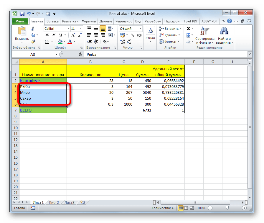
После этого в выделенных ячейках гиперссылки будут удалены, а сам текст останется.
Если вы хотите произвести удаление во всем документе, то сначала наберите на клавиатуре сочетание клавиш Ctrl+A. Этим вы выделите весь лист. Затем, кликнув правой кнопкой мыши, вызывайте контекстное меню. В нём выберите пункт «Удалить гиперссылки».
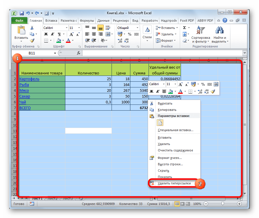
Внимание! Данный способ не подходит для удаления ссылок, если вы связывали ячейки с помощью функции ГИПЕРССЫЛКА.
Способ 4: массовое удаление гиперссылок (версии ранее Excel 2010)
Что же делать, если у вас на компьютере установлена версия ранее Excel 2010? Неужели все ссылки придется удалять вручную? В данном случае тоже имеется выход, хоть он и несколько сложнее, чем процедура, описанная в предыдущем способе. Кстати, этот же вариант можно применять при желании и в более поздних версиях.
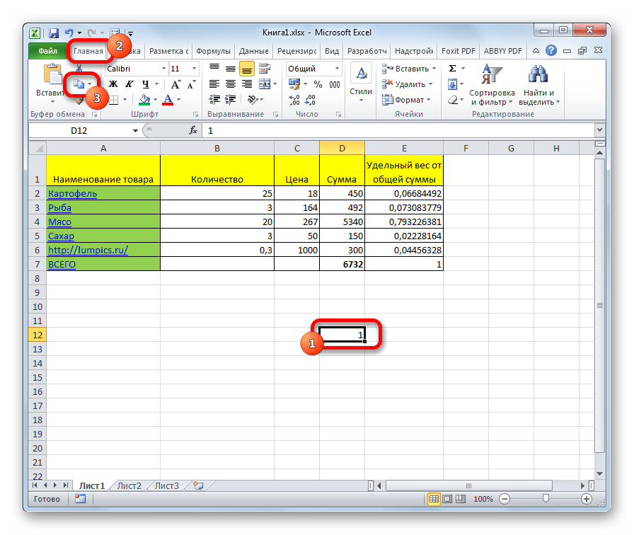
- Выделяем любую пустую ячейку на листе. Ставим в ней цифру 1. Жмем на кнопку «Копировать» во вкладке «Главная» или просто набираем на клавиатуре сочетание клавиш Ctrl+C.
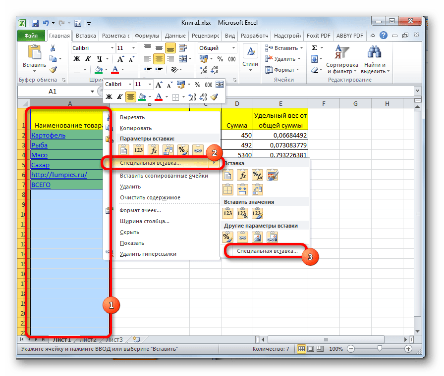
- Выделяем ячейки, в которых расположены гиперссылки. Если вы хотите выбрать весь столбец, то кликните по его наименованию на горизонтальной панели. Если нужно выделить весь лист, наберите сочетание клавиш Ctrl+A. Кликните по выделенному элементу правой кнопкой мыши. В контекстном меню дважды перейдите по пункту «Специальная вставка…».
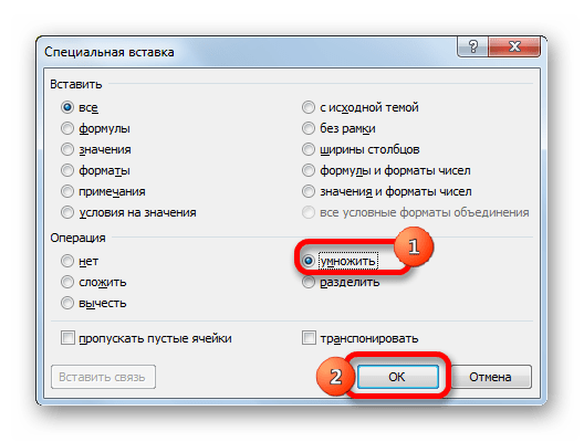
- Открывается окно специальной вставки. В блоке настроек «Операция» ставим переключатель в позицию «Умножить». Жмем на кнопку «OK».
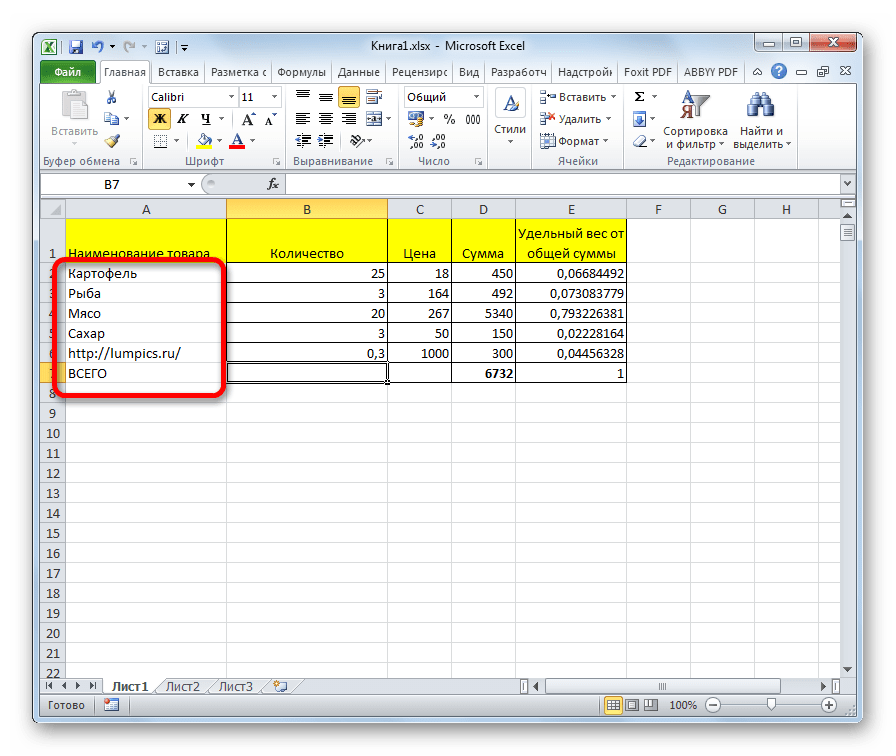
После этого, все гиперссылки будут удалены, а форматирование выделенных ячеек сброшено.
Как видим, гиперссылки могут стать удобным инструментом навигации, связывающим не только различные ячейки одного документа, но и выполняющим связь с внешними объектами. Удаление ссылок легче выполнять в новых версиях Excel, но и в старых версиях программы тоже есть возможность при помощи отдельных манипуляций произвести массовое удаление ссылок.