
Excel for Microsoft 365 Excel for Microsoft 365 for Mac Excel for the web Excel 2021 Excel 2021 for Mac Excel 2019 Excel 2019 for Mac Excel 2016 Excel 2016 for Mac Excel 2013 Excel for Mac 2011 More…Less
This article describes the formula syntax and usage of the DECIMAL
function in Microsoft Excel.
Description
Converts a text representation of a number in a given base into a decimal number.
Syntax
DECIMAL(text, radix)
The DECIMAL function syntax has the following arguments.
-
Text Required.
-
Radix Required. Radix must be an integer.
Remarks
-
The string length of Text must be less than or equal to 255 characters.
-
The Text argument can be any combination of alpha-numeric characters that are valid for the radix, and is not case sensitive.
-
Excel supports a Text argument greater than or equal to 0 and less than 2^53. A text argument that resolves to a number greater than 2^53 may result in a loss of precision.
-
Radix must be greater than or equal to 2 (binary, or base 2) and less than or equal to 36 (base 36).
A radix greater than 10 use the numeric values 0-9 and the letters A-Z as needed. For example, base 16 (hexadecimal) uses 0-9 and A-F, and base 36 uses 0-9 and A-Z. -
If either argument is outside its constraints, DECIMAL may return the #NUM! or #VALUE! error value.
Example
Copy the example data in the following table, and paste it in cell A1 of a new Excel worksheet. For formulas to show results, select them, press F2, and then press Enter. If you need to, you can adjust the column widths to see all the data.
|
Formula |
Description |
Result |
How it works |
|
‘=DECIMAL(«FF»,16) |
Converts the hexadecimal (base 16) value FF to its equivalent decimal (base 10) value (255). |
=DECIMAL(«FF»,16) |
«F» is in position 15 in the base 16 number system. Because all number systems start with 0, the 16th character in hexadecimal will be in the 15th position. The formula below shows how it is converted to decimal: |
|
The HEX2DEC function in cell C3 verifies this result. |
=HEX2DEC(«ff») |
Formula |
|
|
=(15*(16^1))+(15*(16^0)) |
|||
|
‘=DECIMAL(111,2) |
Converts the binary (base 2) value 111 to its equivalent decimal (base 10) value (7). |
=DECIMAL(111,2) |
«1» is in position 1 in the base 2 number system. The formula below shows how it is converted to decimal: |
|
The BIN2DEC function in cell C6 verifies this result. |
=BIN2DEC(111) |
Formula |
|
|
=(1*(2^2))+(1*(2^1))+(1*(2^0)) |
|||
|
‘=DECIMAL(«zap»,36) |
Converts the value «zap» in base 36 to its equivalent decimal value (45745). |
=DECIMAL(«zap»,36) |
«z» is in position 35, «a» is in position 10, and «p» is in position 25. The formula below shows how it is converted to decimal. |
|
Formula |
|||
|
=(35*(36^2))+(10*(36^1))+(25*(36^0)) |
Top of Page
Need more help?
Purpose
Convert a number in a different base to a decimal number
Usage notes
The DECIMAL function converts a number in a known base into its decimal number equivalent. For example, the DECIMAL function can convert the binary number 1101 into the decimal number 13. The number provided to DECIMAL should be a text string.
The DECIMAL function takes two arguments: number and radix. Number should be the text representation of a number in a known base. Radix is the number of digits used to represent numbers (i.e. the base) and should be an integer between 2 and 36. The characters given in number need to conform to the numbering system specified with radix.
Examples
In the hexadecimal number system, the number 255 is represented as «FF». To convert the text string «FF» to the decimal number 255, you can use the DECIMAL function like this:
=DECIMAL("FF",16) // returns 255
To convert the binary number 1101 to its decimal number equivalent, 13, use DECIMAL like this:
=DECIMAL("1101",2) // returns 13
In the example shown, the numbers in column B are in different bases, and the base is given in column C. The formula in column D5 is:
=DECIMAL(B5,C5) // returns 3
As the formula is copied down, the DECIMAL function converts each number in column B to its decimal equivalent using the base specified in column C for the radix argument. The decimal numbers in column D are the output from DECIMAL.
BASE function
The BASE function performs the opposite conversion as the DECIMAL function:
=BASE(100,2) // returns "1100100"
=DECIMAL("1100100",2) // returns 100
See more on the BASE function here.
Number system characters
Different bases use different alphanumeric characters to represent numbers. The table below shows the characters uses for binary, octal, decimal, and hexadecimal number systems.
| Name | Base | Alphanumeric characters |
|---|---|---|
| binary | 2 | 0 — 1 |
| octal | 8 | 0 — 7 |
| decimal | 10 | 0 — 9 |
| hexadecimal | 16 | 0 — 9 and A — F |
Notes
- The number argument should be provided as a text string.
- The result from DECIMAL is a numeric value.
- If number is negative, DECIMAL returns a #NUM! error.
- if number contains a decimal value, DECIMAL returns a #NUM! error.
- If number is out-of-range for the given base, DECIMAL returns a #NUM! error.
In this article, we will learn about how to use the DECIMAL function in Excel.
DECIMAL function in excel is used to convert text representation of numbers of a given base to decimal numbers (base =10).
The table shown below shows you some of the most used base & their radix Alpha — numeric characters
| Base | radix | Alpha-Numeric Characters |
| Binary | 2 | 0 — 1 |
| Octal | 8 | 0 — 7 |
| decimal | 10 | 0 — 9 |
| hexadecimal | 16 | 0 — 9 & A — F |
| hexatridecimal | 36 | 0 — 9 & A — Z |
The DECIMAL function converts the number of a given radix to a number of radix 10 (decimal).
Syntax:
=DECIMAL (number, radix)
Number : value to be converted to decimal.
Radix : or base of the given number. Range from 2 to 36 (integers).
The decimal value is obtained from the number of radix 2 as shown in the above gif.
Let’s understand this function using it in an example.

The numbers & their Radix or base value. We need to convert these numbers to decimal value which is base 10.
Use the formula:
=DECIMAL (A2, B2)
A2 : number
B2 : radix or base
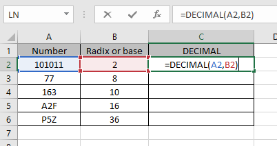
Values to the DECIMAL function is provided as cell reference.

The decimal representation of 101011 of base 2 is 43 of base 10.
Now copy the formula to other cells using the Ctrl + D shortcut key.
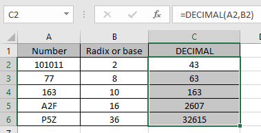
As you can see here the decimal representation of the numbers from the numbers.
Notes:
- The argument to the function can be given as text in quotes or cell reference. Numbers can be given as argument to the function directly without quotes or cell reference.
- The number must be an Alpha numeric number to the given radix or base.
- The function returns the #NUM! Error
- If radix is less than 2 or greater than 36.
- If the argument to the function is not readable by excel.
- The number characters exceed by 255.
- The function returns the # VALUE! Error
- If the text argument exceeds the character limit of 255.
- If the radix integers is non — numeric.
- Radix must be an integer greater than or equal to 2 and less than equal to 36.
- Text argument to the function is not case sensitive.
Hope you understood how to use DECIMAL function and referring cell in Excel. Explore more articles on Excel mathematical conversion functions here. Please feel free to state your query or feedback for the above article.
Popular Articles:
50 Excel Shortcuts to Increase Your Productivity
How to use the VLOOKUP Function in Excel
How to use the COUNTIF in Excel 2016
How to use the SUMIF Function in Excel
Change Separators from Commas to Decimals or Decimals to Commas in Microsoft Excel
by Avantix Learning Team | Updated November 23, 2021
Applies to: Microsoft® Excel® 2013, 2016, 2019 and 365 (Windows)
Depending on your country or region, Excel may display decimal points or dots instead of commas for larger numbers. The decimal point (.) or comma (,) is used as the group separator in different regions in the world. You can change commas to decimal points or dots or vice versa in your Excel workbook temporarily or permanently. The default display of commas or decimal points is based on your global system settings (Regional Settings in the Control Panel) and Excel Options.
If you want to use a decimal point instead of a comma as a group or thousands separator, which is different from your Regional Settings, this can lead to issues with your Excel calculations.
Excel recognizes numbers without group or thousands separators so these separators are actually a format.
Your Regional Settings in your Control Panel on your device are used by default by Excel to determine if decimals should be a period or dot (used in the US and in English Canada for example) or if decimals are a comma (used in many European countries and French Canada).
Recommended article: 10 Great Excel Pivot Table Shortcuts
Do you want to learn more about Excel? Check out our virtual classroom or live classroom Excel courses >
Changing commas to decimals by changing global system settings
It’s important to enter data in Excel in accordance with your global system settings in the Control Panel. For example, if you enter the number 1045.35 and your system is set with US as the region, the period is used as the decimal separator. If you enter the number 1045,35 in France, the comma is used as the decimal separator based on system settings with France as the region.
Below is the Control Panel in Windows 10:

To change the Regional Settings in the Control Panel in Windows 10:
- In the Start a search box on the bottom left of the screen, type Control Panel. The Control Panel appears.
- Click Clock and Region. This may appear as Languages and Regional Standards.
- Below Region, click Change Date, Time, or Number Formats. A dialog box appears. If you change the region, Excel (and other programs) will use settings based on the selected region so US would use periods as decimals and commas as thousands separators.
- If you don’t want to change the region, click Additional settings. A Customize Format dialog box appears.
- Click the Numbers tab.
- Select the desired options in Decimal symbol and Digit grouping symbol. You can also change other options in this dialog box (such as the format of negatives).
- Click OK twice.
Below is the Customize Format dialog box:

Keep in mind that this will change defaults on your device for all Excel workbooks (as well as other programs like Microsoft Access or Microsoft Project). If another user opens the workbook on a different device, the separators will display based on their system settings.
Changing commas to decimals and vice versa by changing Excel Options
You can also change Excel Options so that commas display as the group or thousands separator instead of decimals and vice versa. This option will affect any workbook you open after you have made this change.
To change Excel Options so that commas display as the thousands separator and decimals appear as the decimal separator (assuming your global settings in Regional Settings are set in the opposite way):
- Click the File tab in the Ribbon.
- Click Options.
- In the categories on the left, click Advanced.
- Uncheck Use system separators in the Editing area.
- In the Decimal separator box, enter the desired character such as a decimal or period (.).
- In the Thousands separator box, enter the desired character such as a comma (,).
- Click OK.
Below is the Options dialog box where Use system separators has been turned off and a decimal and comma have been entered as separators:

You may want to change the Options back to Use system separators when you have finished your task.
Creating a formula to change separators and format using current system separators
Another alternative is to write a formula in another cell or column to convert separators. This works well if the data is text with separators that are not used in the current system settings. If you write a formula to convert text to numbers, you can keep the original values as well. In Excel 2013 or later, you can use the NUMBERVALUE function to convert the text to numbers.
The NUMBERVALUE function has the following arguments:
Text – The text to convert to a number.
Decimal_separator – The character used in the original cell to separate the integer and fractional part of the result.
Group_separator – The character used in the original cell to separate groupings of numbers, such as thousands from hundreds and millions from thousands.
The function is entered as follows:
=NUMBERVALUE(Text,Decimal_separator, Group_separator)
For example, if you have 2.500.300,00 in A1 and your device is set to US in the Regional Settings, you could enter the following formula in B1:
=NUMBERVALUE(A1,»,»,».»)
The value that is returned will normally appear as a number without formatting. You can then apply appropriate formatting by pressing Ctrl + 1 and using Format Cells to apply formatting with system separators.
Changing separators using Flash Fill
Flash Fill is a utility that is available in Excel 2013 and later versions and can be used to clean up and / or reformat data. It is not a formula, so if the original data changes, you’ll need to rerun Flash Fill.
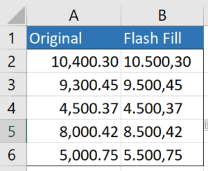
In the example below, the numbers entered in column A are formatted using system settings (US in this case). In column B, we have entered sample data in B2 and B3 with different separators (periods for the group separator and commas for the decimal separator). It’s usually best to enter a few examples to show Excel the pattern. You’ll need data with a pattern to the left in order to use Flash Fill. Once you have entered a few examples of the pattern in cells to the right of the original data, in the cell below the samples (in this case in cell B4) press Ctrl + E. Flash Fill will fill in the remaining cells until it reaches the end of the data set.
The following example was created using Flash Fill in column B (the data that is filled in column B is text):
For more information, check out How to Use Flash Fill in Excel (4 Ways with Shortcuts).
Changing commas to decimals in an Excel worksheet for a selected range using Replace
You can use the Replace command to replace commas with decimals or vice versa In a range of cells on a worksheet. It’s important to understand that this will change the range of cells to text so you won’t be able to use certain functions like SUM. You may want to replace on a copy of the data.
To change commas to decimals using Replace:
- Select the range of cells in which you want to replace commas with decimals. You may select a range of cells, a column or columns or the entire worksheet.
- Press Ctrl + 1 or right-click and select Format Cells. A dialog box appears.
- Click the Number tab.
- In the categories on the left, click Text and then click OK. Notably, the data will be text not numbers.
- Click the Home tab in the Ribbon and in the Editing group, click Find & Select. A drop-down menu appears.
- Click Replace. Alternatively, press Ctrl + H. A dialog box appears.
- In the Find and Replace dialog box, click the Replace tab.
- In the Find what box, enter a comma (the character that you want to find).
- In the Replace with box, enter a decimal or period (the character that you want to replace).
- Click Replace All if you are sure that you want to replace all symbols or characters in the selected range. Click Replace if you want to find and replace one by one in the selected range. Click Find All if you want to find all of the characters to be replaced first and then decide if you want to replace all. Click Find Next if you want to find characters one by one and decide if you want to replace each character by clicking Replace. After replacing all characters, Excel displays a dialog box with the number of replacements.
Below is the Find and Replace dialog box with a comma (,) entered in the Find what box and a decimal (.) in the Replace with box:

In the previous example, only commas were changed to decimals but you may have data that has both commas and decimals (like 1,475.55). In this case, you would need to Replace multiple times.
To change commas to decimals and decimals to commas using Replace:
- Select the range of cells in which you want to replace commas with decimals and decimals with commas. You may select a range of cells, a column or columns or the entire worksheet.
- Press Ctrl + 1 or right-click and select Format Cells. A dialog box appears.
- Click the Number tab.
- In the categories on the left, click Text and then click OK. Notably, the data will be text not numbers.
- Click the Home tab in the Ribbon and in the Editing group, click Find & Select. A drop-down menu appears.
- Click Replace. Alternatively, press Ctrl + H. A dialog box appears.
- In the Find and Replace dialog box, click the Replace tab.
- In the Find what box, enter a decimal.
- In the Replace with box, enter an asterisk (*).
- Click Replace All if you are sure that you want to replace all symbols or characters in the selected range. Click Replace if you want to find and replace one by one in the selected range. Click Find All if you want to find all of the characters to be replaced first and then decide if you want to replace all. Click Find Next if you want to find characters one by one and decide if you want to replace each character by clicking Replace. After replacing all characters, Excel displays a dialog box with the number of replacements.
- In the Find what box, enter a comma.
- In the Replace with box, enter a decimal or period.
- Click Replace All if you are sure that you want to replace all symbols or characters in the selected range. Click Replace if you want to find and replace one by one in the selected range. Click Find All if you want to find all of the characters to be replaced first and then decide if you want to replace all. Click Find Next if you want to find characters one by one and decide if you want to replace each character by clicking Replace. After replacing all characters, Excel displays a dialog box with the number of replacements.
- In the Find what box, enter an asterisk (*).
- In the Replace with box, enter a comma.
- Click Replace All if you are sure that you want to replace all symbols or characters in the selected range. Click Replace if you want to find and replace one by one in the selected range. Click Find All if you want to find all of the characters to be replaced first and then decide if you want to replace all. Click Find Next if you want to find characters one by one and decide if you want to replace each character by clicking Replace. After replacing all characters, Excel displays a dialog box with the number of replacements.
Again, the result will be text, not numbers.
Subscribe to get more articles like this one
Did you find this article helpful? If you would like to receive new articles, join our email list.
More resources
How to Convert Text to Numbers in Excel
How to Highlight Errors, Blanks and Duplicates in Excel Worksheets
3 Excel Strikethrough Shortcuts to Cross Out Text or Values in Cells
How to Replace Blank Cells in Excel with Zeros (0), Dashes (-) or Other Values
Use Conditional Formatting in Excel to Highlight Dates Before Today (3 Ways)
Related courses
Microsoft Excel: Intermediate / Advanced
Microsoft Excel: Data Analysis with Functions, Dashboards and What-If Analysis Tools
Microsoft Excel: Introduction to Power Query to Get and Transform Data
Microsoft Excel: New and Essential Features and Functions in Excel 365
Microsoft Excel: Introduction to Visual Basic for Applications (VBA)
VIEW MORE COURSES >
Our instructor-led courses are delivered in virtual classroom format or at our downtown Toronto location at 18 King Street East, Suite 1400, Toronto, Ontario, Canada (some in-person classroom courses may also be delivered at an alternate downtown Toronto location). Contact us at info@avantixlearning.ca if you’d like to arrange custom instructor-led virtual classroom or onsite training on a date that’s convenient for you.
Copyright 2023 Avantix® Learning
Microsoft, the Microsoft logo, Microsoft Office and related Microsoft applications and logos are registered trademarks of Microsoft Corporation in Canada, US and other countries. All other trademarks are the property of the registered owners.
Avantix Learning |18 King Street East, Suite 1400, Toronto, Ontario, Canada M5C 1C4 | Contact us at info@avantixlearning.ca
Numbers can be represented in a base from 2 to 36. While working with Excel, we are able to convert a number from any base to a base of 10. This step by step tutorial will assist all levels of Excel users in converting a number to its decimal value by using the DECIMAL function.
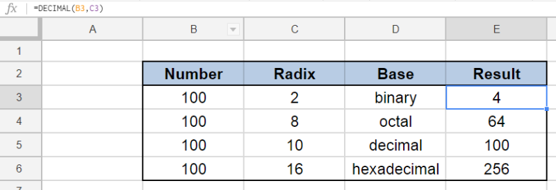 Figure 1. Final result: Excel DECIMAL function
Syntax of DECIMAL Function
DECIMAL converts any value into its decimal value; converts a value in any base to a base of 10
=DECIMAL(number,radix)
- number – the number we want to convert to its decimal value
- radix – the base of the value we want to convert to decimal; the base can be an integer from 2 to 36
Below table shows the alphanumeric characters for some common bases used in Excel:
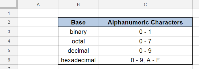 Figure 2. Base and corresponding alphanumeric characters
Setting up our Data
Our data consists of four columns: Number (column B), Radix (column C), Base (column D) and Result (column E). We want to convert the number “100” in four different bases (2, 8, 10 and 16) into its decimal value.
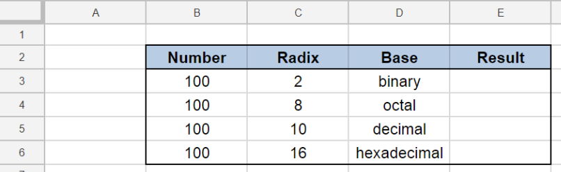 Figure 3. Sample data to convert to decimal value
Convert to decimal value
We want to determine the decimal value of the number “100” in different bases by using the DECIMAL function. Let us follow these steps:
Step 1. Select cell E3
Step 2. Enter the formula: =DECIMAL(B3,C3)
Step 3. Press ENTER
Step 4: Copy the formula in cell E3 to cells E4:E6 by clicking the “+” icon at the bottom-right corner of cell E3 and dragging it down
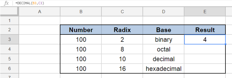 Figure 4. Using the DECIMAL function to convert to decimal value
The value in B3 “100” is a binary number with a base of 2. Its resulting decimal value in E3 is “4”.
For the succeeding examples, the numbers are converted to their corresponding decimal values in cells E4to E6. Note that different bases for the same number, in this case “100”, return different decimal values.
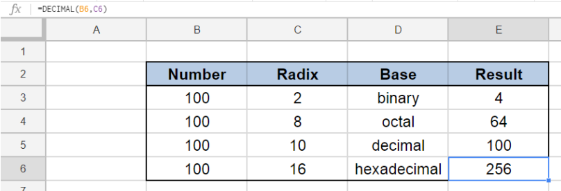 Figure 5. DECIMAL returns different results for different bases
The DECIMAL function can be used to convert any number with a base from 2 to 36 into its decimal value.
Note, however, that the DECIMAL function returns a #NUM! error when the value we want to convert contains characters that are not valid representations of the given base. In our example below, “22” is not a valid binary representation because binary numbers contain only the digits 0 and 1.
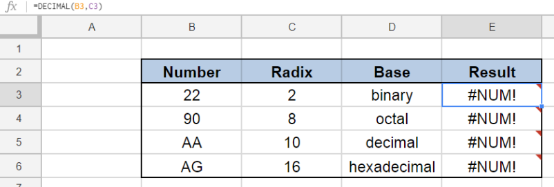 Figure 6. DECIMAL returns error value for invalid characters
Most of the time, the problem you will need to solve will be more complex than a simple application of a formula or function. If you want to save hours of research and frustration, try our live Excelchat service! Our Excel Experts are available 24/7 to answer any Excel question you may have. We guarantee a connection within 30 seconds and a customized solution within 20 minutes.