
Содержание
- Create a new workbook
- Create a workbook
- Create a workbook from a template
- Open a new, blank workbook
- Base a new workbook on an existing workbook
- Base a new workbook on a template
- Need more help?
- How to Create, Write and Read text file in Excel using VBA FileSystemObject
- Tools you can use
- How to create a CSV file
- Example spreadsheet data
- Creating a CSV file
- Notepad (or any text editor)
- Microsoft Excel
- OpenOffice Calc
- Google Docs
- How to Create Workbooks in Excel
- Table of Contents
- Excel 2013 Workbooks
- Make Data-driven Strategic Decisions
- Creating a Blank Excel Workbook
- Create a Workbook from an Excel Template
- Open an Existing Excel Workbook
- Business Scenarios
- Native and Non-Native Files
- Connecting or Importing External Files
- Business Scenarios
- Excel Worksheet Operations
- Change Worksheet Tab Color
- Hide and Unhide Excel Worksheet
- Business Scenarios
- Search and Replace Data
- GoTo and Named Box
- Business Scenarios
- Hyperlinks
- Business Scenarios
- Modifying Workbook Theme
- Become Expert-Level in SQL, R, Python & More!
- Modifying Page Setup
- Insert and Delete Columns and Rows
- Modify Row Height and Column Width
- Hide and Unhide Columns and Rows
- Business Scenarios
- Insert Header and Footers
- Customize Headers and Footers
- Business Scenarios
- Land a High-Paid Business Analyst Job
- Data Validation
- Warning Messages for Data Validation
- Business Scenarios:
- Enable Developer Tab
- Macron Security Options
- Record Macros
- Business Scenarios
- Backward Compatibility
- Workbook Views
- Zoom for Excel Workbooks
- Freeze Panes
- Split Window
- Business Scenarios
- You’re Steps Away from a Business Analyst Job
- Show Formulas
- Business Scenarios
- Add Values to Excel Workbook Properties
- Business Scenarios
- Save Workbooks in Alternate File Formats
- Set the Print Area for an Excel Workbook
- Business Scenarios
- Save Workbooks to Remote Location
- Key Takeaways
- Conclusion
- About the Author
- Recommended Programs
Create a new workbook
A workbook is a file that contains one or more worksheets to help you organize data. You can create a new workbook from a blank workbook or a template.

Create a workbook
Select Blank workbook or press Ctrl+N.
Create a workbook from a template
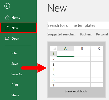
Select File > New.
Double-click a template.
Click and start typing.
Open a new, blank workbook
Click the File tab.
Under Available Templates, double-click Blank Workbook.
Keyboard shortcut To quickly create a new, blank workbook, you can also press CTRL+N.
By default, a new workbook contains three worksheets, but you can change the number of worksheets that you want a new workbook to contain.
You can also add and remove worksheets as needed.
For more information about how to add or remove worksheets, see Insert or delete a worksheet.
Base a new workbook on an existing workbook
Click the File tab.
Under Templates, click New from existing.
In the New from Existing Workbook dialog box, browse to the drive, folder, or Internet location that contains the workbook that you want to open.
Click the workbook, and then click Create New.
Base a new workbook on a template
Click the File tab.
Do one of the following:
To use one of the sample templates that come with Excel, under Available Templates, click Sample Templates and then double-click the template that you want.
To use a recently used template, click Recent Templates, and then double-click the template that you want.
To use your own template, on the My Templates, and then on the Personal Templates tab in the New dialog box, double-click the template that you want.
Note: The Personal Templates tab lists the templates that you have created. If you do not see the template that you want to use, make sure that it is located in the correct folder. Custom templates are typically stored in the Templates folder, which is usually C:Usersuser_nameAppDataLocalMicrosoftTemplates in Windows Vista, and C:Documents and Settingsuser_nameApplication DataMicrosoftTemplates in Microsoft Windows XP.
Tip: To obtain more workbook templates, you can download them from Microsoft Office.com. In Available Templates, under Office.com Templates, click a specific template category, and then double-click the template that you want to download.
Need more help?
You can always ask an expert in the Excel Tech Community or get support in the Answers community.
Источник
How to Create, Write and Read text file in Excel using VBA FileSystemObject
Tools you can use
Here’s a list of articles in this blog that explains how to use the FileSystemObject for various operations.
1) Quickly get or extract filenames from FilePaths in Excel using VBA Macro: Let’s assume, you have a list of filepaths in one of the columns in your excel sheet and you want extract only filenames from each given file path and write the name of the file in the next column.
2) How to copy or move files from one folder to another in Excel using VBA: The example in this articles explains how easily you can move files across various folders using the methods from VBAs FileSystemObject.
One the easiest way to write and read a text file in Excel is by using the TextStream object in VBA. This is how you will actually define a TextStream object.
Dim objTS As TextStream
Before defining it, you’ll have to reference Microsoft Scripting Library in your VBA application.
Once defined, you will have access to all the methods and properties in the TextStream object. However, you will have to initialize the object with the TextStream object returned by a FileSystemObject method. Like this,
Set objTS = objFso. CreateTextFile (sFolder & «/birds.json»)
Let us see an example.
Open an Excel file and save the file in .xlsm format (it’s the macro format). Press Ctrl + F11 keys to open the VBA editor. From the Project Explorer , double click Sheet1 and write the code.
Note: Instead of a .txt file, I am creating a .json file for my example. The procedure is the same for a .txt file.
After referencing Microsoft Scripting Library, I have defined two objects in beginning.
There are two separate procedures for creating, writing and reading the text file. The text is a JSON array and I am creating JSON file named birds.json .
The CreateTextFile() method of FileSystemObject, returns a TextStream object. And, here I am initializing the TextStream object variable (I have declared in the beginning).
Set objTS = objFso. CreateTextFile (sFolder & «/birds.json»)
The methods WriteLine (to write in the file) and Close are TextStream methods.
The second procedure opens and reads the JSON file (it can be a .txt file). Here again, I am using the OpenTextFile() method of the FileSystemObject to initialize the TextStream object. This time it’s in open mode, so it can read the contents.
Set objTS = objFso. OpenTextFile (sFolder & «/birds.json»)
Run a simple Do While until it reaches the end the stream (or file). The “ReadLine” method will read each line in the file and write in the debug window. Along will AtEndOfStream property, you can use the AtEndOfLine property.
Don’t forget to close the instance of the file, after performing an operation.
Источник
How to create a CSV file

CSV is a simple file format used to store tabular data, such as a spreadsheet or database. Files in the CSV format can be imported to and exported from programs that store data in tables, such as Microsoft Excel or OpenOffice Calc.
CSV stands for «comma-separated values». Its data fields are often separated, or delimited, by a comma.
Example spreadsheet data
For example, let’s say you had a spreadsheet containing the following data.
| Name | Class | Dorm | Room | GPA |
|---|---|---|---|---|
| Sally Whittaker | 2018 | McCarren House | 312 | 3.75 |
| Belinda Jameson | 2017 | Cushing House | 148 | 3.52 |
| Jeff Smith | 2018 | Prescott House | 17-D | 3.20 |
| Sandy Allen | 2019 | Oliver House | 108 | 3.48 |
The above data could be represented in a CSV-formatted file as follows:
Here, the fields of data in each row are delimited with a comma and individual rows are separated by a newline.
Creating a CSV file
A CSV is a text file, so it can be created and edited using any text editor. More frequently, however, a CSV file is created by exporting (File > Export) a spreadsheet or database in the program that created it. Click a link below for the steps to create a CSV file in Notepad, Microsoft Excel, OpenOffice Calc, and Google Docs.
Notepad (or any text editor)
To create a CSV file with a text editor, first choose your favorite text editor, such as Notepad or vim, and open a new file. Then enter the text data you want the file to contain, separating each value with a comma and each row with a new line.
Save this file with the extension .csv. You can then open the file using Microsoft Excel or another spreadsheet program. It would create a table of data similar to the following:
| Title1 | Title2 | Title3 |
| one | two | three |
| example1 | example2 | example3 |
In the CSV file you created, individual fields of data were separated by commas. But what if the data itself has commas in it?
If the fields of data in your CSV file contain commas, you can protect them by enclosing those data fields in double quotes («). The commas that are part of your data are kept separate from the commas which delimit the fields themselves.
For example, let’s say that one of our text fields is a user-created description that allows commas in the description. If our data looked like this:
| Lead | Title | Phone | Notes |
| Jim Grayson | Senior Manager | (555)761-2385 | Spoke Tuesday, he’s interested |
| Prescilla Winston | Development Director | (555)218-3981 | said to call again next week |
| Melissa Potter | Head of Accounts | (555)791-3471 | Not interested, gave referral |
To retain the commas in our «Notes» column, we can enclose those fields in quotation marks. For instance:
As you can see, only the fields that contain commas are enclosed in quotes.
The same goes for newlines which may be part of your field data. Any fields containing a newline as part of its data need to be enclosed in double quotes.
If your fields contain double quotes as part of their data, the internal quotation marks need to be doubled so they can be interpreted correctly. For instance, given the following data:
| Player | Position | Nicknames | Years Active |
|---|---|---|---|
| Skippy Peterson | First Base | «Blue Dog», «The Magician» | 1908-1913 |
| Bud Grimsby | Center Field | «The Reaper», «Longneck» | 1910-1917 |
| Vic Crumb | Shortstop | «Fat Vic», «Icy Hot» | 1911-1912 |
We can represent it in a CSV file as follows:
Here, the entire data field is enclosed in quotes, and internal quotation marks are preceded (escaped by) an additional double quote.
Here are the rules of how data should be formatted in a CSV file, from the IETF’s document, RFC 4180. In these examples, «CRLF» represents a carriage return and a linefeed (which together constitute a newline).
- Each record (row of data) is to be on a separate line, delimited by a line break. For example:
The last record in the file may or may not have an ending line break. For example:
There may be an optional header line appearing as the first line of the file with the same format as normal record lines. The header contains names corresponding to the fields in the file. Also, it should contain the same number of fields as the records in the rest of the file. For example:
In the header and each record, there may be one or more fields, separated by commas. Each line should contain the same number of fields throughout the file. Spaces are considered part of a field and should not be ignored. The last field in the record must not be followed by a comma. For example:
Each field may or may not be enclosed in double quotes. If fields are not enclosed with double quotes, then double quotes may not appear inside the fields. For example:
Fields containing line breaks (CRLF), double quotes, and commas should be enclosed in double quotes. For example:
If double quotes enclose fields, then a double quote appearing inside a field must be escaped by preceding it with another double quote. For example:
Microsoft Excel
To create a CSV file using Microsoft Excel, launch Excel and then open the file you want to save in CSV format. For example, below is the data contained in our example Excel worksheet:
| Item | Cost | Sold | Profit |
|---|---|---|---|
| Keyboard | $10.00 | $16.00 | $6.00 |
| Monitor | $80.00 | $120.00 | $40.00 |
| Mouse | $5.00 | $7.00 | $2.00 |
| Total | $48.00 |
Once open, click File and choose Save As. Under Save as type, select CSV (Comma delimited) or CSV (Comma delimited) (*.csv), depending on your version of Microsoft Excel.
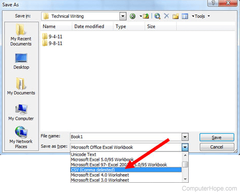
After you save the file, you are free to open it up in a text editor to view it or edit it manually. Its contents resemble the following:
The last row begins with two commas because the first two fields of that row were empty in our spreadsheet. Don’t delete them — the two commas are required so that the fields correspond from row to row. They cannot be omitted.
OpenOffice Calc
To create a CSV file using OpenOffice Calc, launch Calc and open the file you want to save as a CSV file. For example, below is the data contained in our example Calc worksheet.
| Item | Cost | Sold | Profit |
|---|---|---|---|
| Keyboard | $10.00 | $16.00 | $6.00 |
| Monitor | $80.00 | $120.00 | $40.00 |
| Mouse | $5.00 | $7.00 | $2.00 |
| Total | $48.00 |
Once open, click File, choose the Save As option, and for the Save as type option, select Text CSV (.csv) (*.csv).
If you were to open the CSV file in a text editor, such as Notepad, it would resemble the example below.
As in our Excel example, the two commas at the beginning of the last line make sure the fields correspond from row to row. Do not remove them!
Google Docs
Open Google Docs and open the spreadsheet file you want to save as a CSV file. Click File, Download as, and then select CSV (current sheet).
Источник
How to Create Workbooks in Excel

Table of Contents
From a birds eye view, Microsoft Excel, is a software program that is a part of the Microsoft Office suite, used to create spreadsheets. However, excel with it’s spreadsheets has done wonders in the world of business analytics. And in this tutorial we will learn the A to Z of Microsoft excel, with a heavy emphasis on creating and managing workbooks and worksheets.
Excel 2013 Workbooks
The Microsoft (MS) Excel workbook is a file within the MS Excel application, where one can enter and store data. A workbook contains multiple worksheets. Each worksheet is a combination of a number of cells that hold information pertaining to a particular subject and can be modified as per the requirements.В
A workbook defines the data that is contained within the worksheet. However, the manipulation of data happens only through worksheets (not workbooks). In Excel 2013, each workbook has a separate window. It becomes easier to work on workbooks or two monitors at the same time as the name of the workbook is displayed in the title bar.
Usually, we can create a new workbook when we start a new project. There are several ways to create a workbook in Excel 2013
- Create a workbook with a blank document
- Create a workbook from a template
- Open an existing workbook
Make Data-driven Strategic Decisions

Creating a Blank Excel Workbook
Excel 2013 allows users to create a new workbook from a blank document. There is also an option to create a new workbook based on the existing workbook. By default, a new workbook contains three worksheets. However, we can change the number of worksheets in a workbook as per the requirements.
Create a Workbook from an Excel Template
A template is a pre-designed worksheet which could be modified to suit users’ needs. The Excel template contains predefined formulas and custom formatting. This saves a lot of time and effort while working on a new project.
To create a workbook from a template, we need to select an appropriate template, as per the requirements. Besides Microsoft, there are many individual users as well as third-party providers to create customized templates.
Open an Existing Excel Workbook
An existing workbook is one that has been previously saved and stored in the computer or on the web. One can open existing workbooks from local computer drives, Skydrive, online storage and other online storage places. Skydrive is a Microsoft product, and anyone can sign in or register on Skydrive for storing files online.
Business Scenarios
John has been assigned the task of creating an inventory data sheet for his company’s assets. To do this, he has to work extensively on Microsoft Excel 2013. He needs to enter and edit data in workbooks, starting with creating a workbook.
Let us take a look at the overview of the steps for opening an Excel workbook.
- To create a new worksheet, open Microsoft Excel and click the File tab.
- Click New and then click the Blank Workbook option.
- To create a workbook from a template, under New, click the Search for Online Templates search bar and enter the type of template required
- Click the Search icon.
- Select any of the available Templates and click Create.
- To open an existing workbook, click File, then click Open.
- Click Computer and then click Browse.
- In the open pop-up window, navigate to the Excel file you want to open, select it and click open.
Native and Non-Native Files
Let us first understand what Native and Non-Native files are.
- The type of file format that each software program can create or accept is called native files.
- A software program that allows us to work and save files in a different format is called non-native files.
Some popular native file format in Excel 2013:
- Excel Workbook(XLSX): It is the default XML based file format from Excel 2007 — 2013 versions.
- Excel Workbook (XLS): It is the default file format from Excel 1997- 2003 version.
- Excel Binary Workbook(XLSB): It is the binary file format for Excel 2007 to 2013
- Excel Workbook Code(XLSM): It is the XML based and macro-enabled file format for Excel 2007 to 2013.
- Excel Workbook Code(XLM): It is the macro-enabled file format for earlier versions of Excel. There are Excel workbook templates XLTS, XML data(XML) and Excel Addin(XLAM).
Some popular non-native file format used in Excel 2013 are
- text(.txt): It allows the user to save a workbook as a tab-delimited text file. The user can save this file as Macintosh and MS-DOS operating system compatible.
- Comma Separated Values (csv):В Allows a user to save a workbook as a comma delimited text file. The User can save this while as Macintosh and MS-DOS operating system compatible.
Connecting or Importing External Files
In Excel 2013, the main advantage of connecting to external data is a periodic analysis of this data without repeatedly copying it. Repeated copying is time-consuming and an error-prone process. By default connections to external data may be disabled on the computer. If we want to use this feature, we need to first enable the external data connections from trust center settings.
There are two ways of importing data:
- Delimited: This option is used when the text contains the comma, tab, semicolon and other symbols.
- Fixed Width: This option is used when all the rows have similar text length.
In Excel 2013 we can connect or import data from the following sources:
- From Access: This option allows for easy access to data from MS Access databases that store huge information. Once the link to the access database has been registered in MS Excel then any information changes in the access database will result in automatic updating of the Excel file.
- From the Web:В This option allows for access to data from websites such as share markets and live currency converters. It is a time-consuming task to copy the data from the website to MS Excel. Excel allows for easy import of external data from the website.
- From Text Files: This option allows for access to text format files as supported in many operating systems. There are some other popular data sources in Excel to connect or import data for analysis including SQL server, analysis services, windows zero marketplace and Microsoft query.
External data can be imported in a number of ways.
- Table: This is a general table format where the data will be imported in rows and columns.
- Pivot Table Report: A pivot table reports is a summary of raw data in a table format. If we select this option, the data will be imported in a pivot table form.
- Pivot Chart: A pivot chart represents data series, categories, and chart access the same way as a standard chart. It also allows us to filter controls right on the chart so we can quickly analyze a subset of the data.
- Power View Report. Power view report is an interactive data exploration, visualization and presentation experience that encourage intuitive, ad hoc reporting.
- Only Create Connection: Creates a connection between the data source and the Excel file.
Business Scenarios
John has been assigned the task of taking an inventory of his company’s data assets. He will have to use data from non-Excel files, as well. He wants to import text files into Excel 2013. He also wants to explore the Get External Data option in Excel. Let us have an overview of the steps for importing files into Excel workbook.
- To open a non-native file in Excel, click the open item under the file tab.
- Click computer and then browse.
- In the open pop-up window, navigate to the required folder, then select all files in the files of type Combo box.
- Select the required .txt or .csv file and click open.
- In the text import wizard, select the appropriate options, click next, then click finish.
- To import external files click the data tab.
- Select the from text option.
- In the import text from the pop-up window, select the required text file and click Import.
- Complete the steps in the Text import wizard and click finish.
- In the import data dialogue box, choose the destination for the imported text and click OK.
- Use the refresh all item under the Data tab to import any changes made to a text file.
Excel Worksheet Operations
An Excel Worksheet contains different rows and columns. The intersection of a row and column is a cell. Various options can be performed using a worksheet.
- Insert: This option allows us to insert a new worksheet to an existing workbook.
- Delete: This option allows us to delete selected worksheets from a current workbook.
- Rename: This option permits us to rename the worksheet.
- Move or Copy: This option allows us to move or copy a worksheet from one workbook to another workbook. You can also change the order of worksheet, using this functionality.
- View Code: This option allows us to view VBA macro code in the selected worksheet.
- Protect Sheet: This option allows us to lock or password protects the worksheet.
- Tab Color: This option allows us to color the worksheet tab.
- Hide: This option allows us to hide selected worksheets in the current workbook.
- Unhide: This option allows us to unhide worksheets in the current workbook.
- Select All Sheets: This option allows us to delete, move or copy workbooks to another worksheet.
Change Worksheet Tab Color
In Excel 2013, different worksheet tabs can be differentiated by the use of different tab colors. If sheet tabs have been color-coded, the sheet tab name will be underlined in the user-specified color when selected. If the sheet tab is displayed with a background color, then the sheet has not been selected.
Hide and Unhide Excel Worksheet
Sometimes, we may want to hide certain worksheets for security and later unhide when required. For instance, while creating a dashboard for the top management to review, we can easily hide the rule data worksheet. When worksheets are hidden, there is no effect on formulas.
All Worksheets in a workbook can be hidden, but at least one worksheet needs to be visible.
Business Scenarios
To create and collate employee data, John has to work with multiple worksheets at a time. To be able to manage multiple worksheets, John wants to use the worksheet Tab Color and Hide/Unhide options. Let us have an overview of the steps for using tab color and hide/Unhide in Excel workbook.
- Right-click the worksheet tab to open the context menu.
- To change the tab color, select the Tab color menu item and select color.
- To hide a worksheet, right click on the worksheet tab and select the hidden menu.
- To unhide a worksheet, right click on the worksheet tab and select the unhide menu.
- To view the worksheet again, click to select the hidden worksheet and click OK.
Search and Replace Data
You can search for data and replace old data with new data in Excel 2013. This feature is very useful to search and replace data in multiple records instead of moving from one cell to another to make changes. This function also saves a lot of time and effort.
GoTo and Named Box
GoTo and named box features in Excel can be used to quickly move to different cells in a worksheet. This feature is useful when we’re working on a large set of data. The GoTo and Named Box functionality can be used to select named cells and a specific data range in a worksheet. The GoTo function allows us to select all comments, Constants, Formulas, Visible cells, conditional format, and blank cells in a worksheet.
Business Scenarios
The marketing department has now been renamed the Online Marketing department. John has been assigned the task of changing this in the employee data sheet. He wants to complete this task using the Find and Replace tool in Excel 2013. While managing the employee data records, John has to navigate through large worksheets in Excel. He wants to explore easier ways of navigating a worksheet, such as GoTo and Name Box.
Let us have an overview of the steps used to Find and Replace in Excel workbook.
- To find and replace a particular entry in an Excel worksheet, click the find and select menu in the editing group on the home tab.
- Select the Replace item.
- In the Find and replace the pop-up window, type the value to be found in the find what field.
- Select the required .txt or .csv file and click open.
- Type the value that will replace the current value in the Replace with field and click OK.
- Close the find and replace the pop-up window.
- To navigate to a particular row and column, select the GoTo option in the Find and select menu.
- In the reference field, type the column and row to jump to and click OK.
For worksheets with a lot of data, select the column reference first in the GoTo pop-up window, and then jump to the row using the Name box.
Hyperlinks
Hyperlinks enable quick access to other files, documents, and Excel workbooks via links. The hyperlinks that we add to the Excel Worksheets can be of the following types:
- Existing file or Web page: This option allows us to hyperlink a web page or an existing file. We can also link pictures, videos, audio and other file formats.
- Place in this document: This option allows us to place a hyperlink in the document. Once clicked on the cell, it jumps to the hyperlinked cell or worksheet.
- Create a New Document: This option allows us to create new documents when clicked on the hyperlinked cell.
- Email Address: This option allows us access to the specific email address so that we can send out an email by clicking the hyperlink cell.
Business Scenarios
John is preparing an invoice template for the purchasing department. He needs to provide a link to a particular web page within the template for reference. This can be done by inserting hyperlinks. Let us look at the steps used to insert hyperlinks in Excel workbook.
- Select the desired cell to insert a hyperlink.
- Right click on the selected cell.
- Click the hyperlink from the drop-down menu.
- Type the URL in the address bar of the insert a hyperlink pop-up window.
- Click OK.
- Click the hyperlink to open the webpage.
A hyperlink can also be created to an existing document or a place in the current document.
Modifying Workbook Theme
By default, in Excel 2013 every workbook uses an office theme. A workbook theme has a unique sense of colors, fonts, and effects. These themes are shared across MS office programs so that all the official documents can have a uniform look. You can browse for themes, customize them based on the requirements, or even save the current theme and apply it to other workbooks.
This feature allows us to change color and style with the selection of a single theme. Also, in case any changes are done in the cells, styles, and color, they will be applied automatically throughout the workbook.
Become Expert-Level in SQL, R, Python & More!
Modifying Page Setup
A worksheet sometimes contains a large amount of data or even multiple charts. If we want to print worksheet or workbooks, we first need to fine tune the page setup options.
Margins: This option allows us to change or modify margins preferences based on our requirements. Some of the options it allows are:
- Default settings or Normal
- Wide and Narrow
- Orientation: This option allows us to change or modify the orientation of the workbook layout to portrait or landscape view.
- Size: This option allows us to change the paper size for printing. It also allows us to select different types of paper sizes.
- Print Area: This option allows us to set a print area or clear prints area.
- Breaks: This option allows us to set page breaks for workbooks.
- Backgrounds: This option allows us to set the background of our workbook to a picture from local disc or from the web.
- Print Titles: This option allows us to print only titles available in the Workbook.
Insert and Delete Columns and Rows
In a worksheet, we can insert and delete columns or rows. Columns are labeled from A to XFD, whereas the rows are labeled from 1 to 1048576. Below are the shortcut keys to insert and delete columns or rows:
- Shift + SpaceBar: Allows us to select the entire row.
- Control +В Spacebar: Allows us to select the entire column.
- Control + or (-): Allows us to select rows or columns that need to be deleted in a workbook.
- Control + shift + +: Allows us to insert columns or rows.
- Clear Content Option: Allows us to clear the cell contents.
Modify Row Height and Column Width
In Excel 2013, by default, each row, height and column width is set to the same measurement. We can change the row height and column width in several ways, such as text wrap and cell merge.
Sometimes we need to manually change the row, height and column with the displaying cell contents clearly, or use autofit the content. The row height value can be changed between 0 to 249 and column width value can be changed between 0 to 255.
Hide and Unhide Columns and Rows
Sometimes, we may want to compare certain rows or columns without changing the structure of the worksheet, or by removing a row or column temporarily instead of deleting them permanently. Microsoft Excel has a feature that allows us to temporarily hide a row or column from view.
Business Scenarios
After looking at the employee data table, John’s manager has asked him to change the theme of the worksheet. He has also asked John to delete the SSN column and insert a new column to add the employees work timing details. Also, John has to hide the earnings data when the table is displayed to others without deleting the column. Let us look at the steps used to perform the above tasks in the Excel workbook.
- To change the theme, click the page layout tab and select the required theme under the themes drop-down.
- To add a column, identify the column where a new column needs to be inserted.
- Right-click on the selected column, select from the right-click context menu.
- To delete a column, select the column to be deleted, right-click and click to select Delete.
- To insert a row, identify a row where a new row needs to be inserted.
- Right-click on the selected row, select insert from the right-click context menu.
- To delete a row, select the row to be deleted, right-click and click to delete.
- To hide a column, select the required column, right-click and click to hide.
- To unhide the column, select the columns on either side of the hidden column, right-click and click to select unhide.
- To hide a row, select the required row, right-click and click to select.
- To unhide the row, select the row above and the row below the hidden row, right-click and click to select unhide.
- To change the row height, select the row, click format and click to select row height.
- In the row height pop-up window, type in the required size and click OK.
- To change the column width, select the column, click format and click to select column width.
- In the column width pop-up window, type in the required size and click OK.
Microsoft Excel 2013 allows us to customize a worksheet by adding headers and footers. We can add pictures, page numbers, copyright information, date, time elements in headers and footers of a worksheet. Generally, this information is inserted for printing purposes.В
Headers and footers are not displayed on the worksheet in the normal view and displayed only in page layout view and on printed pages.
- Different First Page: This option allows us to differentiate the first page of the worksheet with a different header and footer
- Different Odd and Even Pages: This option allows us to differentiate the header and footers for odd pages and even pages.
- Scale with Documents: This option allows us to scale the header and footer to fit the document.
- Align with Page Margins: This option allows us to align all the pages of the document with margins for printing.
Business Scenarios
John is preparing an invoice for the purchasing department. He needs to add the time, page number and company name in the header and footer of every sheet in the invoice.
Let us look at the steps used to perform the above tasks in Excel workbook.
- Click the header and footer under the insert tab.
- Click the current date from the design tab.
- Click the GoTo footer icon.
- Click the page number icon from the design tab.
- Click the Number of pages icon from Design Tab.
- Click the GoTo header icon.
- Click the first grid and type the desired text. Then press Enter so that text is displayed.
Land a High-Paid Business Analyst Job
Data Validation
Data validation is an Excel feature that allows us to restrict the data entered in a cell. We can prevent invalid user entry’s through data validation. This feature allows us to enter invalid data but warns us when we try to type it in the cell and provides custom messages to define what type of data the user can enter into the cell. This function also provides instructions guiding users to enter correct entries.В
Data Validation is used mainly for creating common templates or workbooks to work with multiple users for storing accurate and consistent data. By using data validation, we can prevent invalid user entries through set rules. Below of elevation rules with equal to, between, minimum and maximum values.
- Whole number: This option allows users to enter only integers. As per software programming. Whole numbers are called integers.
- Decimal: This option allows users to enter only decimal values.
- List: This option allows users to display a list of items as a dropdown in cells.
- Date: This option allows users to restrict date entries.
- Time: This option allows users to restrict time entries.
- Text Length: This option allows users to enter text based on the validation rule.
- Custom: This option allows users to customize options by using formulas or functions to create a validation rule.
Warning Messages for Data Validation
Data Validation will show the default input and alert messages to users. An input message to guide users on the type of data that should be entered in the cells. This message appears near the cell. There are three types of error alert messages displayed to the users when they enter invalid data:
- Stop: This message prevents users from entering invalid data into a cell with two options. Retry to edit the invalid entry or cancel to remove the invalid entry.
- Warning: This message warns, or alerts users when an invalid entry is made with three options.
- Yes — to accept the invalid entry
- No — To edit the invalid entry
- Cancel — To remove the invalid entry
- Information: This message informs users when an invalid entry is made with two options.
- OK — To accept the invalid value
- Cancel — To remove the invalid entry
Business Scenarios:
John is collecting the details of new employees in his company. He wants to restrict the data that would be entered in a cell so that the employees enter the correct details. John performs this using the data validation option. Let us look at the steps used to perform the above tasks in Excel workbook.
- Select a cell and click data validation from the data tab
- Select text length from the combo box.
- Select Equal to, from the data combo box and type the limit in the length box and click OK.
- To customize the input message, select a cell and click data validation under the data tab.
- Click the input message tab from the data validation pop-up window and type the messages.
- To customize error alert messages click Error Alert tab and enter the message.
- Select warning from style combo box.
- Click OK.
Enable Developer Tab
In Excel 2013, the Developer tab is not enabled by default, but we need to set it up to use the features given below:
Write Macros in the visual basic editor to automate tasks. Run macros that were previously recorded or written. Use XML commands to work with XML data. Insert and use form and Active X controls. Create applications to use with Microsoft office programs.В
Macron Security Options
When we open a workbook, we can change the macro security settings to control which macro to run and under what circumstance. There are several macro security settings options:
- Disable all macros without notification: If this is set as the default setting, then all macros in the document as well as the security alert, are disabled.
- Disable all macros with notification: If this is set as a default setting, then all macros in the document are disabled, and the security alert will be notified.
- Disable all macros except digitally signed macros: If this is set as a default setting, then all the macros in the document except the digitally signed macros as well as the security alert, get disabled without notification. This function is similar to disabling all macros with notification options.
- Enable all macros: Not recommended as potentially dangerous code can run. If this is the default setting, all macros in the document will run without any alerts.
- Trust Access to the VBA project object model: If this is the default setting, it provides a security code that will automate an office program and programmatically change the Microsoft visual basic for applications, VBA environment, and the object model.
Record Macros
Macros are a set of directions or instructions for Excel to automate a task to be performed in a particular worksheet with a simple click of a button. A micro recorder registers all the steps required to complete the transaction that we want the macro to perform.
These steps can include typing text or numbers, clicking cells or commands on the ribbon or on menus, formatting, selecting cells, rows or columns and dragging the mouse to select cells on the worksheet.
- Macro Name: Key in a proper macro name and follow the below rules for setting the name for macros.
- Rule 1: Do not use two words for the macro name.
- Rule 2: Do not use application of built-in keywords for macro name.
- Rule 3: Macro name should not start with special characters, symbols and numerical.
- Assign Shortcut Keys: You can assign shortcut keys, the macro, as per our requirements, but it is not mandatory.
- Store Macro: By default, Macros will be stored in the workbook where we are recording or writing code. If we want to store macros in a new workbook, we need to change this option, and if we want to run macros in all workbooks, select a personal macro workbook.
- Description: we can provide a description for each micro to help other users understand the macro, but it is not mandatory.
Business Scenarios
John has been assigned the task of highlighting the earnings of the employees in the accounts department in an Excel workbook. Along with the employee details, he wants to explore the use of macro details to do this.
Let us look at the steps used to perform the above tasks in Excel workbook.
- Click options item in the file tab.
- Click the customize ribbon.
- Select the Developer checkbox to add the Developer tab to the ribbon and click OK.
- Click macro security on the Developer tab.
- Select the enable all macros(not recommended; potentially dangerous code can run) radio button and click OK.
- Click Record macro item on the Developer tab. Right-click on the selected row, select insert from right-click context menu.
- Enter the required details in the record macro pop-up window.
- Perform the tasks to be recorded in the macro.
- Click stop recording item.
- Click macros in the view tab.
- Select view macros.
- Select this workbook for macros in.
- Select the macro name
- Click Run.
Backward Compatibility
Backward compatibility means checking the compatibility with earlier models or earlier versions of the same product. A new version of the program is said to be backward compatible if it uses files and data created by an older version of the same program. Backward compatibility is important, as it enables easy exchange and accessibility of data irrespective of the Excel version in use.
In general, manufacturers are trying to keep all their products backward compatible. However, at times we need to sacrifice the backward compatibility feature in any product to take advantage of new technology. In Excel 2013, we can check the backward compatibility for earlier versions in three ways.
- Inspect Document: This option allows checking for hidden properties of the workbook or personal information if any.
- Check Accessibility: This option allows checking for the accessibility of the workbook content to people with disabilities.
- Check Compatibility: This option allows checking for compatibility of the workbook features to work with earlier versions of Excel.
Excel applications have only backward compatibility which means the latest versions of Excel features cannot be used in the earlier versions of Excel.
Workbook Views
In Excel 2013, by default, workbook views are said to be normal, and sometimes we need to change based on the requirements. Excel application contains four types of workbook views.
- Normal: Displays the ruler and allows for data to be entered into cells for insertion of charts and pictures into the worksheet
- Page Break View: Displays the workbook with page breaks and page numbers to adjust work with content to print.
- Page Layout: Displays the workbook as pages with rulers, displays headers, and footers. It is primarily used for printing purposes.
- Custom View: Allows us to change workbooks using custom zoom options. Once this option is set and we open the workbook, it will automatically zoom the world book according to the given specifications.
Zoom for Excel Workbooks
If the workbook contains huge data and does not display all the content in the window, we can use the zoom feature. We can zoom in and zoom out with a camera to increase the size of an object in the camera’s viewer. Zoom option is found at the bottom right corner, next to the workbook view icons.
- Zoom Out: Click on this option to decrease workbook, zoom Size, and the minimum zoom level is 10%.
- Zoom In: Click on this option to increase workbook zoom size and max zoom
Freeze Panes
Sometimes, if our workbook contains a lot of content and is difficult to compare sections, in Excel 2013, we have an option called freeze panes that works in three ways as listed below.
- Freeze Panes: This option allows the rows and columns to be visible to rest of the worksheet, based on the current range selection, even while strolling up and down the worksheet.
- Freeze Top Row: This option allows top row visibility and is preferred when the top road contains any headers.
- Freeze First Column: This option allows first column visibility and is preferred when the first column contains any headers.
To unfreeze the rows or columns, click the freeze panes command and then select unfreeze panes from the drop-down menu.
Split Window
Sometimes, we may need to compare different sections of the same workbook without creating a new window. In such cases, we can use the split window functionality. This command allows us to divide the worksheet content into four parts with scroll bars and increase or decrease the window size.
Business Scenarios
John is working with a lot of data in Excel. He needs to scroll down and view rows of data, but when he reaches the bottom of the screen, the column is named in the top row disappear. Also, he has not been able to view the entire data sheet from left to right. To view all part of the data sheets, he wants to use freeze panes and split window features in Excel 2013. Let us look at the steps used to perform the above tasks in Excel workbook.
- To freeze a row or column, click the view tab.
- Click the freeze panes items in the windows group.
- Click the freeze top row or freeze first column item.
- To unfreeze a row or column, click to select unfreeze panes from the freeze panes drop-down menu.
- To divide the window into different panes that each scroll separately, click split on the view tab.
- To remove the dissection, click split again.
You’re Steps Away from a Business Analyst Job
Show Formulas
In Excel, by default, we can see formula result in cells and sometimes we may need to see which cells contain formulas. By using the show formulas feature, we can see the formulas in all the cells instead of the formula result. This feature allows us to quickly read through all formulas to check for errors.
Business Scenarios
The HR team has sent an earning summary to John. He has been asked to check the formula used and verify the calculations. Let us look at the steps used to perform the above tasks in Excel workbook.
- Select the cell whose formula has to be viewed.
- On the Formulas tab, select Show Formulas and verify them.
Add Values to Excel Workbook Properties
In Excel 2013, by default, a workbook author is the name of the person who created the workbook. It is usually one name, however, at times, a workbook may have several authors and requires adding other author’s names to the workbook. We can add additional author information, such as title, tanks and comments, status, category subject, hyperlink base company name and manager of the author.
Business Scenarios
The HR team has sent an employee report to John. He has been asked to add a title and tag to the workbook so that it would be easier to organize and retrieve the workbook.
Let us look at the steps used to perform the above tasks in the Excel workbook.
- Click the file tab.
- Type appropriate entries in the title and tag text boxes.
- Click shows all properties to view the entire workbook properties.
Save Workbooks in Alternate File Formats
In Excel 2013, by default, workbooks will be saved with XLXS file extension, and we can save a workbook in alternate file formats as listed below.
- PDF: Portable Document Format.
- XPS: XML paper specification: Allows us to easily print a workbook. For instance, if we don’t have access to the printer and someone else does, but they don’t have the Excel application installed in their system, this file format comes to our rescue.
- Text(txt): Saves a workbook as a tab-delimited text file. Text files of the most widely compatible format for data. They can’t be opened and viewed on any computer. They’re usually called .txt files.
- Comma Separated Values(CSV): Saves a workbook as a comma delimited text file. Comma-separated value files are a kind of text files which do not store formatting information as contained in the original worksheet. They’re usually called .CSV files.
Set the Print Area for an Excel Workbook
Sometimes we need to print a worksheet, which contains huge amounts of data. In this case, Excel allows us to set up a print area. This option allows us to set a print area based on our requirements and clear the print area if it is not required. We can print workbooks in three ways:
- Prince Active Sheets: This option allows us to prince only active worksheet content.
- Print Entire Workbook: This option allows us to print entire workbook content.
- Print Selection: This option allows us to print only the selected area of a worksheet. Prince area of a worksheet can be sent using the page break view mode.
Business Scenarios
After looking at the employee data table, John’s manager has asked him to print the employee_code, Last_Name, first_name, SSN, and Region columns. John needs to set the prince area to print these. Let us look at the steps used to perform the above tasks in Excel workbook.
- Select the columns/area to be printed
- Click the page layout tab and click the print area item
- From the drop-down menu, select the print area menu item
- Click OK to continue
- Click the file tab and click to select print
- Click the print icon
- To clear the print area, click the black arrow to go back
- Click print area item again
- Click the clear print area menu item
Save Workbooks to Remote Location
In Excel 2013, we have several options for sharing workbooks online. We can save the file on the cloud, publish a link, share the file through several social media platforms, or send it by email. We can save Excel files on the cloud and share it using Windows SkyDrive.В
SkyDrive is an online storage space hosted by Microsoft. The advantage of using the cloud space is that we can access the files from anywhere and from any device. However, we can use Skydrive only if we have a Microsoft account.
Key Takeaways
Here’s a quick summary of the Excel 13 workbook and worksheet tutorial:
- MS Excel Workbook is a file within the MS Excel application where one can enter and store data. A workbook can be created from an existing workbook or from a blank document.
- Macros are a set of directions or instructions for Excel to automate a task to be performed in a particular worksheet with a simple click of a button.
- Excel application contains four types of workbook views – normal, page break view, page layout and a custom view.
- Excel worksheets can be saved to .pdf, .txt, and .csv formats. This feature ensures compatibility with other operating systems.
- SkyDrive is an MS product that is used to store files online so that it can be accessed from anywhere.
Conclusion
Creating and managing workbooks and worksheets is an essential part of excel 2013. And now that you have learned it, you might wish to master excel, or take another leap forward, and step into business analytics. With Simplilearn’s Business Analytics for Strategic Decision Making with IIT Roorkee, you will not just be able to master excel, but other BI tools like, Tableau, Power BI, Jira and various other tools too! Enroll now, and start your journey to becoming a successful business intelligence professional now
Simplilearn is one of the world’s leading providers of online training for Digital Marketing, Cloud Computing, Project Management, Data Science, IT, Software Development, and many other emerging technologies.
Recommended Programs
Business Analytics for Strategic Decision Making with IIT Roorkee
Источник
Create a workbook in Excel
Excel makes it easy to crunch numbers. With Excel, you can streamline data entry with AutoFill. Then, get chart recommendations based on your data, and create them with one click. Or easily spot trends and patterns with data bars, color coding, and icons.
Create a workbook
-
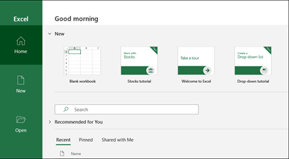
Open Excel.
-
Select Blank workbook.
Or press Ctrl+N.
Enter data
To manually enter data:
-
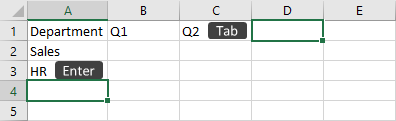
Select an empty cell, such as A1, and then type text or a number.
-
Press Enter or Tab to move to the next cell.
To fill data in a series:
-
Enter the beginning of the series in two cells: such as Jan and Feb; or 2014 and 2015.
-
Select the two cells containing the series, and then drag the fill handle
 across or down the cells.
 across or down the cells.

Next:
Save your workbook to OneDrive
Need more help?
![]()
Download Article
![]()
Download Article
Do you need to create a spreadsheet in Microsoft Excel but have no idea where to begin? You’ve come to the right place! While Excel can be intimidating at first, creating a basic spreadsheet is as simple as entering data into numbered rows and lettered columns. Whether you need to make a spreadsheet for school, work, or just to keep track of your expenses, this wikiHow article will teach you everything you know about editing your first spreadsheet in Microsoft Excel.
-
1
Open Microsoft Excel. You’ll find it in the Start menu (Windows) or in the Applications folder (macOS). The app will open to a screen that allows you to create or select a document.
- If you don’t have a paid version of Microsoft Office, you can use the free online version at https://www.office.com to create a basic spreadsheet. You’ll just need to sign in with your Microsoft account and click Excel in the row of icons.
-
2
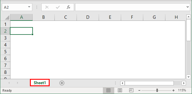
Click Blank workbook to create a new workbook. A workbook is the name of the document that contains your spreadsheet(s). This creates a blank spreadsheet called Sheet1, which you’ll see on the tab at the bottom of the sheet.
- When you make more complex spreadsheets, you can add another sheet by clicking + next to the first sheet. Use the bottom tabs to switch between spreadsheets.
Advertisement
-
3
Familiarize yourself with the spreadsheet’s layout. The first thing you’ll notice is that the spreadsheet contains hundreds of rectangular cells organized into vertical columns and horizontal rows. Some important things to note about this layout:
- All rows are labeled with numbers along the side of the spreadsheet, while the columns are labeled with letters along the top.
- Each cell has an address consisting of the column letter followed by the row number. For example, the address of the cell in the first column (A), first row (1) is A1. The address of the cell in column B row 3 is B3.
-
4
Enter some data. Click any cell one time and start typing immediately. When you’re finished with that cell, press the Tab ↹ key to move to the next cell in the row, or the ↵ Enter key to the next cell in the column.
- Notice that as you type into the cell, the content also appears in the bar that runs across the top of the spreadsheet. This bar is called the Formula Bar and is useful for when entering long strings of data and/or formulas.[1]
- To edit a cell that already has data, double-click it to bring back the cursor. Alternatively, you can click the cell once and make your changes in the formula bar.
- To delete the data from one cell, click the cell once, and then press Del. This returns the cell to a blank one without messing up the data in other rows or columns. To delete multiple cell values at once, press Ctrl (PC) or ⌘ Cmd (Mac) as you click each cell you want to delete, and then press Del.
- To add a new blank column between existing columns, right-click the letter above the column after where you’d like the new one to appear, and then click Insert on the context menu.
- To add a new blank row between existing rows, right-click the row number for the row after the desired location, and then click Insert on the menu.
- Notice that as you type into the cell, the content also appears in the bar that runs across the top of the spreadsheet. This bar is called the Formula Bar and is useful for when entering long strings of data and/or formulas.[1]
-
5
Check out the functions available for advanced uses. One of the most useful features of Excel is its ability to look up data and perform calculations based on mathematical formulas. Each formula you create contains an Excel function, which is the «action» you’re performing. Formulas always begin with an equal (=) sign followed by the function name (e.g., =SUM, =LOOKUP, =SIN). After that, the parameters should be entered between a set of parentheses (). Follow these steps to get an idea of the type of functions you can use in Excel:
- Click the Formulas tab at the top of the screen. You’ll notice several icons in the toolbar at the top of the application in the panel labeled «Function Library.» Once you know how the different functions work, you can easily browse the library using those icons.
- Click the Insert Function icon, which also displays an fx. It should be the first icon on the bar. This opens the Insert Function panel, which allows you to search for what you want to do or browse by category.
- Select a category from the «Or select a category» menu. The default category is «Most Recently Used.» For example, to see the math functions, you might select Math & Trig.
- Click any function in the «Select a function» panel to view its syntax, as well as a description of what the function does. For more info on a function, click the Help on this function.
- Click Cancel when you’re done browsing.
- To learn more about entering formulas, see How to Type Formulas in Microsoft Excel.
-
6
Save your file when you’re finished editing. To save the file, click the File menu at the top-left corner, and then select Save As. Depending on your version of Excel, you’ll usually have the option to save the file to your computer or OneDrive.
- Now that you’ve gotten the hang of the basics, check out the «Creating a Home Inventory from Scratch» method to see this information put into practice.


Advertisement
-
1
Open Microsoft Excel. You’ll find it in the Start menu (Windows) or in the Applications folder (macOS). The app will open to a screen that allows you to create or open a workbook.
-
2
Name your columns. Let’s say we’re making a list of items in our home. In addition to listing what the item is, we might want to record which room it’s in and its make/model. We’ll reserve row 1 for column headers so our data is clearly labeled. [2]
.- Click cell A1 and type Item. We’ll list each item in this column.
- Click cell B1 and type Location. This is where we’ll enter which room the item is in.
- Click cell C1 and type Make/Model. We’ll list the item’s model and manufacturer in this column.
-
3
Enter your items on each row. Now that our columns are labeled, entering our data into the rows should be simple. Each item should get its own row, and each bit of information should get its own cell.
- For example, if you’re listening the Apple HD monitor in your office, you may type HD monitor into A2 (in the Item column), Office into B2 (in the Location column), and Apple Cinema 30-inch M9179LL into B3 (the Make/Model column).
- List additional items on the rows below. If you need to delete a cell, just click it once and press Del.
- To remove an entire row or column, right-click the letter or number and select Delete.
- You’ve probably noticed that if you type too much text in a cell it’ll overlap into the next column. You can fix this by resizing the columns to fit the text. Position the cursor on the line between the column letters (above row 1) so the cursor turns into two arrows, and then double-click that line.
-
4
Turn the column headers into drop-down menus. Let’s say you’ve listed hundreds of items throughout your home but only want to view those stored in your office. Click the 1 at the beginning of row 1 to select the whole row, and then do the following:
- Click the Data tab at the top of Excel.
- Click Filter (the funnel icon) in the toolbar. Small arrows now appear on each column header.
- Click the Location drop-down menu (in B1) to open the filter menu.
- Since we just want to see items in the office, check the box next to «Office» and remove the other checkmarks.
- Click OK. Now you’ll only see items the selected room. You can do this with any column and any data type.
- To restore all items, click the menu again and check «Select All» and then OK to restore all items.
-
5
Click the Page Layout tab to customize the spreadsheet. Now that you’ve entered your data, you may want to customize the colors, fonts, and lines. Here are some ideas for doing so:
- Select the cells you want to format. You can select an entire row by clicking its number, or an whole column by clicking its letter. Hold Ctrl (PC) or Cmd (Mac) to select more than one column or row at a time.
- Click Colors in the «Themes» area of the toolbar to view and select color theme.
- Click the Fonts menu to browse for and select a font.
-
6
Save your document. When you’ve reached a good stopping point, you can save the spreadsheet by clicking the File menu at the top-left corner and selecting Save As.


Advertisement
-
1
Open Microsoft Excel. You’ll find it in the Start menu (Windows) or in the Applications folder (macOS). The app will open to a screen that allows you to create or open a workbook.
- This method covers using a built-in Excel template to create a list of your expenses. There are hundreds of templates available for different types of spreadsheets. To see a list of all official templates, visit https://templates.office.com/en-us/templates-for-excel.
-
2
Search for the «Simple Monthly Budget» template. This is a free official Microsoft template that makes it easy to calculate your budget for the month. You can find it by typing Simple Monthly Budget into the search bar at the top and pressing ↵ Enter in most versions.
-
3
Select the Simple Monthly Budget template and click Create. This creates a new spreadsheet from a pre-formatted template.
- You may have to click Download instead.
-
4
Click the Monthly Income tab to enter your income(s). You’ll notice there are three tabs (Summary, Monthly Income, and Monthly Expenses) at the bottom of the workbook. You’ll be clicking the second tab. Let’s say you get income from two companies called wikiHow and Acme:
- Double-click the Income 1 cell to bring up the cursor. Erase the content of the cell and type wikiHow.
- Double-click the Income 2 cell, erase the contents, and type Acme.
- Enter your monthly income from wikiHow into the first cell under the «Amount» header (the one that says «2500» by default). Do the same with your monthly income from «Acme» in the cell just below.
- If you don’t have any other income, you can click the other cells (for «Other» and «$250») and press Del to clear them.
- You can also add more income sources and amounts in the rows below those that already exist.
-
5
Click the Monthly Expenses tab to enter your expenses. It’s the third tab at the bottom of the workbook. Those there are expenses and amounts already filled in, you can double-click any cell to change its value.
- For example, let’s say your rent is $795/month. Double-click the pre-filled amount of «$800,» erase it, and then type 795.
- Let’s say you don’t have any student loan payments to make. You can just click the amount next to «Student Loans» in the «Amount» column ($50) and press Del on your keyboard to clear it. Do the same for all other expenses.
- You can delete an entire row by right-clicking the row number and selecting Delete.
- To insert a new row, right-click the row number below where you want it to appear, and then select Insert.
- Make sure there are no extra amounts that you don’t actually have to pay in the «Amounts» column, as they’ll be automatically factored into your budget.
-
6
Click the Summary tab to visualize your budget. Once you’ve entered your data, the chart on this tab will automatically update to reflect your income vs. your expenses.
- If the info doesn’t calculate automatically, press F9 on the keyboard.
- Any changes you make to the Monthly Income and Monthly Expenses tabs will affect what you see in your Summary.
-
7
Save your document. When you’ve reached a good stopping point, you can save the spreadsheet by clicking the File menu at the top-left corner and selecting Save As.


Advertisement
Add New Question
-
Question
How do I name a spreadsheet?

When you click «Save As,» at the bottom of the page there should be a file name box. Whatever you type into that box will be your spreadsheet’s name.
-
Question
Can I rename the columns, instead of A, B, C, etc.?
You cannot change those labels. Typically, the name of the column is simply written in the first row.
-
Question
How do I make more space to type in the boxes?
As you’re typing, select the cell where you want the text to be and select «Wrap Text» at the top of the page. This will contain all of the text to the same cell, which will grow as you type.
See more answers
Ask a Question
200 characters left
Include your email address to get a message when this question is answered.
Submit
Advertisement
Thanks for submitting a tip for review!
About This Article
Article SummaryX
1. Open Excel.
2. Click New Blank Workbook.
3. Enter column headers into row 1.
4. Enter data on individual rows.
5. Click the Page Layout tab to format the data.
6. Click File > Save As to save the document.
Did this summary help you?
Thanks to all authors for creating a page that has been read 2,886,243 times.
Is this article up to date?
Создание файлов Excel методами Workbooks.Add, Worksheet.Copy и текстовых файлов с помощью оператора Open и метода CreateTextFile из кода VBA Excel. Создание документов Word рассмотрено в отдельной статье.
Метод Workbooks.Add
Описание
Файлы Excel можно создавать из кода VBA с помощью метода Add объекта Workbooks.
Workbooks.Add – это метод, который создает и возвращает новую книгу Excel. Новая книга после создания становится активной.
Ссылку на новую книгу Excel, созданную методом Workbooks.Add, можно присвоить объектной переменной с помощью оператора Set или обращаться к ней, как к активной книге: ActiveWorkbook.
Синтаксис
Workbooks.Add (Template)
Template – параметр, который определяет, как создается новая книга.
| Значение Template | Параметры новой книги |
|---|---|
| Отсутствует | Новая книга с количеством листов по умолчанию. |
| Полное имя существующего файла Excel | Новая книга с указанным файлом в качестве шаблона. |
| xlWBATChart | Новый файл с одним листом диаграммы. |
| xlWBATWorksheet | Новый файл с одним рабочим листом. |
Примеры
Пример 1
Создание новой книги Excel с количеством листов по умолчанию и сохранение ее в папку, где расположен файл с кодом VBA:
|
Sub Primer1() ‘Создаем новую книгу Workbooks.Add ‘Сохраняем книгу в папку, где расположен файл с кодом ActiveWorkbook.SaveAs (ThisWorkbook.Path & «Моя новая книга.xlsx») ‘Закрываем файл ActiveWorkbook.Close End Sub |
Файл «Моя новая книга.xlsx» понадобится для следующего примера.
Пример 2
Создание новой книги по файлу «Моя новая книга.xlsx» в качестве шаблона с присвоением ссылки на нее объектной переменной, сохранение нового файла с новым именем и добавление в него нового рабочего листа:
|
1 2 3 4 5 6 7 8 9 10 11 12 13 14 15 16 17 18 |
Sub Primer2() ‘Объявляем объектную переменную с ранней привязкой Dim MyWorkbook As Workbook ‘Создаем новую книгу по шаблону файла «Моя новая книга.xlsx» Set MyWorkbook = Workbooks.Add(ThisWorkbook.Path & «Моя новая книга.xlsx») With MyWorkbook ‘Смотрим какое имя присвоено новому файлу по умолчанию MsgBox .Name ‘»Моя новая книга1″ ‘Сохраняем книгу с новым именем .SaveAs (ThisWorkbook.Path & «Моя самая новая книга.xlsx») ‘Смотрим новое имя файла MsgBox .Name ‘»Моя самая новая книга» ‘Добавляем в книгу новый лист с именем «Мой новый лист» .Sheets.Add.Name = «Мой новый лист» ‘Сохраняем файл .Save End With End Sub |
Метод Worksheet.Copy
Описание
Если в коде VBA Excel применить метод Worksheet.Copy без указания параметра Before или After, будет создана новая книга с копируемым листом (листами). Новая книга станет активной.
Примеры
Пример 3
Создание новой книги с помощью копирования одного листа (в этом примере используется книга, созданная в первом примере):
|
Sub Primer3() ‘Если книга источник не открыта, ее нужно открыть Workbooks.Open (ThisWorkbook.Path & «Моя новая книга.xlsx») ‘Создаем новую книгу копированием одного листа Workbooks(«Моя новая книга.xlsx»).Worksheets(«Лист1»).Copy ‘Сохраняем новую книгу с именем «Еще одна книжица.xlsx» в папку, ‘где расположен файл с кодом ActiveWorkbook.SaveAs (ThisWorkbook.Path & «Еще одна книжица.xlsx») End Sub |
Также, как и при создании нового файла Excel методом Workbooks.Add, при создании новой книги методом Worksheet.Copy, можно ссылку на нее присвоить объектной переменной.
Пример 4
Создание новой книги, в которую включены копии всех рабочих листов из файла с кодом VBA:
|
Sub Primer4() ThisWorkbook.Worksheets.Copy End Sub |
Пример 5
Создание новой книги, в которую включены копии выбранных рабочих листов из файла с кодом VBA:
|
Sub Primer5() ThisWorkbook.Sheets(Array(«Лист1», «Лист3», «Лист7»)).Copy End Sub |
Создание текстовых файлов
Оператор Open
При попытке открыть несуществующий текстовый файл с помощью оператора Open, такой файл будет создан. Новый файл будет создан при открытии его в любом режиме последовательного доступа, кроме Input (только для чтения).
Пример
|
1 2 3 4 5 6 7 8 9 10 11 12 13 14 15 16 17 |
Sub Primer6() Dim ff As Integer, ws As Object ‘Получаем свободный номер для открываемого файла ff = FreeFile ‘Создаем новый текстовый файл путем открытия ‘несуществующего в режиме чтения и записи Open ThisWorkbook.Path & «Мой-новый-файл.txt» For Output As ff ‘Записываем в файл текст Write #ff, «Этот файл создан при его открытии оператором « & _ «Open по несуществующему адресу (полному имени).» ‘Закрываем файл Close ff ‘Открываем файл для просмотра Set ws = CreateObject(«WScript.Shell») ws.Run ThisWorkbook.Path & «Мой-новый-файл.txt» Set ws = Nothing End Sub |
В имени текстового файла пробелы заменены дефисами (знаками минус), так как метод Run объекта Wscript.Shell не способен открывать файлы с именами, содержащими пробелы.
Рекомендую открывать файлы для просмотра методом ThisWorkbook.FollowHyperlink. Пример и преимущества этого метода в статье VBA Excel. Открыть файл другой программы.
Метод FileSystemObject.CreateTextFile
Для создания нового текстового файла из кода VBA Excel по указанному имени, можно использовать метод CreateTextFile объекта FileSystemObject.
Пример
|
Sub Primer7() Dim fso, fl, ws ‘Создаем новый экземпляр объекта FileSystemObject Set fso = CreateObject(«Scripting.FileSystemObject») ‘Присваиваем переменной fl новый объект TextStream, ‘связанный с созданным и открытым для записи файлом Set fl = fso.CreateTextFile(ThisWorkbook.Path & «Еще-один-текстовый-файл.txt») ‘Записываем в файл текст fl.Write («Этот текстовый файл создан методом CreateTextFile объекта FileSystemObject.») ‘Закрываем файл fl.Close ‘Открываем файл для просмотра Set ws = CreateObject(«WScript.Shell») ws.Run ThisWorkbook.Path & «Еще-один-текстовый-файл.txt» End Sub |
Стоит отметить, что новый текстовый файл может быть создан и с помощью метода OpenTextFile объекта FileSystemObject при условии присвоения параметру create значения True.
Create a Spreadsheet in Excel (Table of Content)
- Introduction to Create Spreadsheet in Excel
- How to Create a Spreadsheet in Excel?
Introduction to Create Spreadsheet in Excel
A spreadsheet is a grid-based file designed to manage or perform any calculation on personal or business data. It is the best choice for users because it has 400+ functions and features such as pivot, coloring, graph, chart, and conditional formatting. It is accessible in both Office 365 and MS Office. Office 365 is a cloud-based application, whereas MS Office is an on-premises solution.
The workbook is the Excel lingo for ‘spreadsheet.’ MS Excel uses this term to emphasize that a single workbook can contain multiple worksheets, each with its own data grid, chart, or graph.
How to Create a Spreadsheet in Excel?
Here are a few examples of creating different types of spreadsheets in Excel with the key features of the created spreadsheets.
You can download this Create Spreadsheet Excel Template here – Create Spreadsheet Excel Template
Example #1 – How to Create Spreadsheet in Excel?
Step 1: Open MS Excel.
Step 2: Go to Menu and select New >> Click on the Blank workbook to create a simple worksheet.
OR – Press Ctrl + N: To create a new spreadsheet.
Step 3: By default, Sheet 1 will be created as a worksheet in the spreadsheet. The name of the spreadsheet will be given as Book 1 if you are opening it for the first time.
Key Features of the Created Spreadsheet:
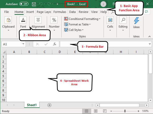
- Basic App Functions Area: There is a green banner that contains all types of actions to perform on the worksheet, like – save the file, back or front step move, new, undo, redo, and many more.
- Ribbon Area: This is a gray area just below the basic app functions area called Ribbon. It contains data manipulation, a data visualizing toolbar, page layout tools, and many more.
- Spreadsheet Work Area: By default, a grid contains alphabetic columns like A, B, C, …, Z, ZA…, ZZ, ZZA… and rows as numbers like 1,2 3, …. 100, 101, and… so on. Each rectangle box in the spreadsheet is called a cell, like the one selected in the above image (cell A1). It is a cell where the user can perform their calculation for personal or business data.
- Formula Bar: It shows the data in the selected cell; if it contains any formula, it will show here. Like the above area, a search bar is available in the top right corner, and a sheet tab is available on the downside of the worksheet. A user can change the name of the sheet name.
Once you create an Excel Spreadsheet, you can convert it to a universally accepted format like PDF. For convenience, some useful Excel to PDF converters converts Excel to PDF files for free while maintaining the original formatting.
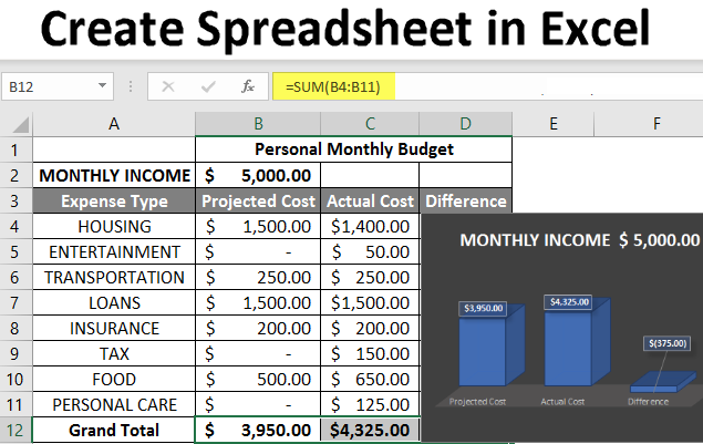
Example #2 – How to Create a Simple Budget Spreadsheet in Excel?
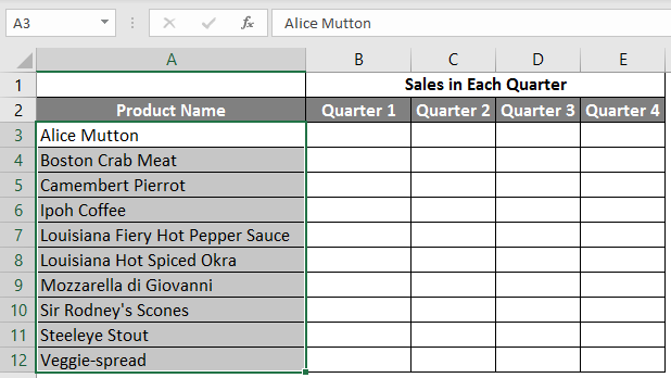
Suppose a user wishes to design a spreadsheet for budget calculation. For 2018, he has a few products and their quarterly sales. He now wants to present his client with this budget.
Let’s see how we can do this with the help of the spreadsheet.
Step 1: Open MS Excel.
Step 2: Go to Menu and select New >> Click on the Blank workbook to create a simple worksheet.
OR – Press Ctrl + N: To create a new spreadsheet.

Step 3: Go to the spreadsheet work area, sheet 1.
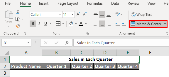
Step 4: Now create headers for Sales in each quarter in the first row by merging cells from B1 to E1. In row 2, give the product name and each quarter’s name.
Step 5: Write down all product names in column A.
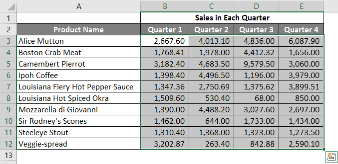
Step 6: Provide the sales data for each quarter before every product.
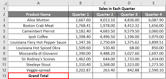
Step 7: In the next row, put one header for Grand Total and calculate each quarter’s total sales.
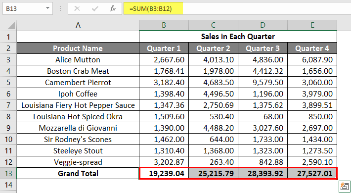
Step 8: Calculate the grand total for each quarter by summation >> apply in other cells in B13 to E13.
Step 9: Let’s convert the sales value into the ($) currency symbol.
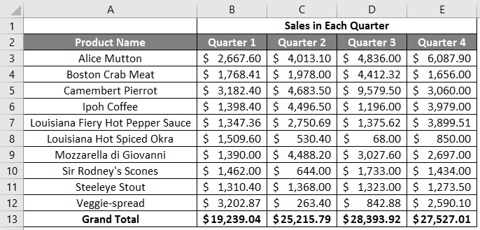
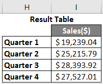
Step 10: Create a Result Table with each quarter’s total sales.
Plot the pie chart to represent the data to the client in a professional way that looks attractive. A user can change the look of the graph by just clicking on it.
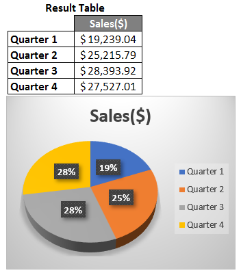
Summary of Example 2: As the user wants to create a spreadsheet to represent sales data to the client, it is done here.
Example #3 – How to Create a Personal Monthly Budget Spreadsheet in Excel?
Let’s assume a user wants to create a spreadsheet to determine their monthly personal budget. For the year 2022, he has estimated costs and actual costs. He now wants to show his family this budget.
Let’s see how we can do this with the help of the spreadsheet.
Step 1: Open MS Excel.
Step 2: Go to Menu and select New >> Click on the Blank workbook to create a simple worksheet.
OR – Press Ctrl + N: To create a new spreadsheet.

Step 3: Go to the spreadsheet work area, Sheet 2.
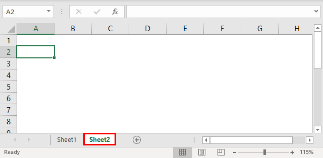
Step 4: Now create headers for Personal Monthly Budget in the first row by merging cells from B1 to D1. In row 2, give MONTHLY INCOME; in row 3, give Expense type, Projected Cost, Actual Cost, and Difference.
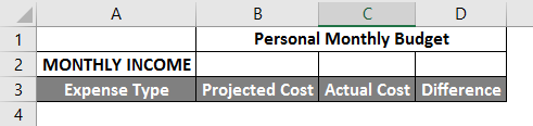
Step 5: Write down all the expenses in column A.
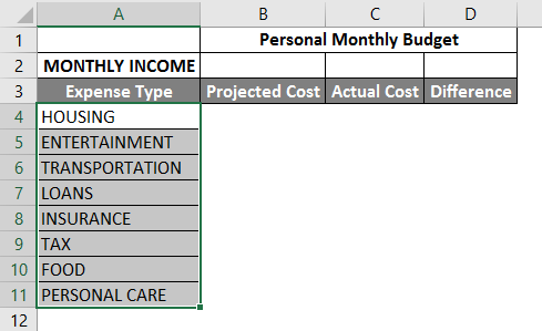
Step 6: Now, provide the monthly income, Projected cost, and Actual Cost data for each expense type.
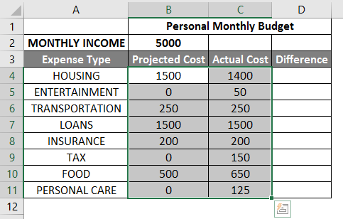
Step 7: In the next row, put one header for Grand Total and calculate the total and difference from the project to the actual cost.
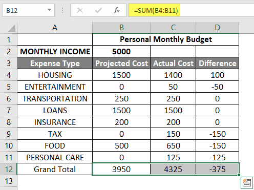
Step 8: Now highlight the header and add boundaries using toolbar graphics. >> The cost and income value in $, so make it by currency symbol.
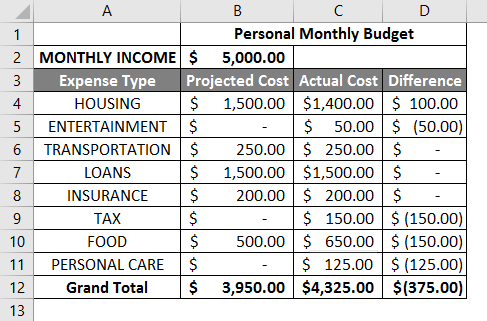
Step 9: Create a Result Table with each quarter’s total sales.
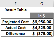
Step 10: Plot the pie chart to represent the data for the family. A user can choose one which he likes.
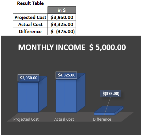
Summary of Example 3: As the user wanted to create a spreadsheet to represent monthly budget data to the family, we have created the same here. The close bracket shows in the data for the negative value.
Things to Remember
- A spreadsheet is a grid-based file designed to manage or perform any calculation on personal or business data.
- It is available in MS Office as well as Office 365.
- The workbook is the Excel lingo for ‘spreadsheet.’ MS Excel uses this term to emphasize that a single workbook can contain multiple worksheets.
How to add data in a spreadsheet Video
Recommended Articles
This article is a comprehensive guide to creating Spreadsheets in Excel. Here we have discussed how to create a Spreadsheet in Excel, examples, and a downloadable Excel template. You may also look at the following articles to learn more –
- Excel Spreadsheet Formulas
- Group Worksheets In Excel
- Excel Spreadsheet Examples
- Worksheets in Excel