
![]()
Download Article
![]()
Download Article
Do you need to create a spreadsheet in Microsoft Excel but have no idea where to begin? You’ve come to the right place! While Excel can be intimidating at first, creating a basic spreadsheet is as simple as entering data into numbered rows and lettered columns. Whether you need to make a spreadsheet for school, work, or just to keep track of your expenses, this wikiHow article will teach you everything you know about editing your first spreadsheet in Microsoft Excel.
-

1
Open Microsoft Excel. You’ll find it in the Start menu (Windows) or in the Applications folder (macOS). The app will open to a screen that allows you to create or select a document.
- If you don’t have a paid version of Microsoft Office, you can use the free online version at https://www.office.com to create a basic spreadsheet. You’ll just need to sign in with your Microsoft account and click Excel in the row of icons.
-
2
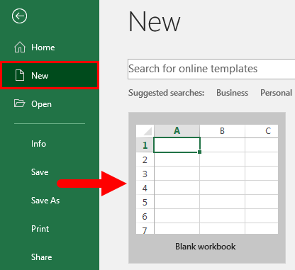
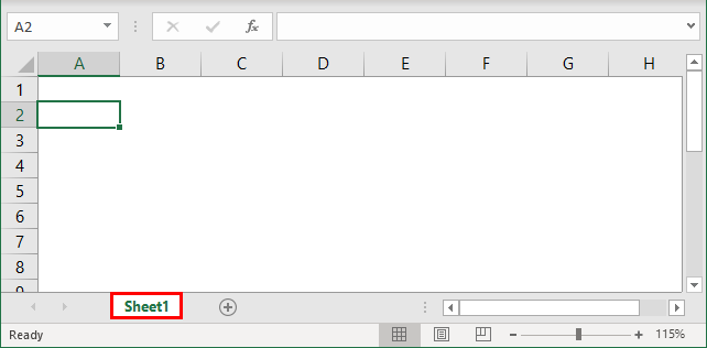
Click Blank workbook to create a new workbook. A workbook is the name of the document that contains your spreadsheet(s). This creates a blank spreadsheet called Sheet1, which you’ll see on the tab at the bottom of the sheet.
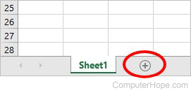
- When you make more complex spreadsheets, you can add another sheet by clicking + next to the first sheet. Use the bottom tabs to switch between spreadsheets.
Advertisement
-
3
Familiarize yourself with the spreadsheet’s layout. The first thing you’ll notice is that the spreadsheet contains hundreds of rectangular cells organized into vertical columns and horizontal rows. Some important things to note about this layout:
- All rows are labeled with numbers along the side of the spreadsheet, while the columns are labeled with letters along the top.
- Each cell has an address consisting of the column letter followed by the row number. For example, the address of the cell in the first column (A), first row (1) is A1. The address of the cell in column B row 3 is B3.
-
4
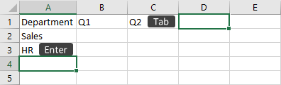
Enter some data. Click any cell one time and start typing immediately. When you’re finished with that cell, press the Tab ↹ key to move to the next cell in the row, or the ↵ Enter key to the next cell in the column.
- Notice that as you type into the cell, the content also appears in the bar that runs across the top of the spreadsheet. This bar is called the Formula Bar and is useful for when entering long strings of data and/or formulas.[1]
- To edit a cell that already has data, double-click it to bring back the cursor. Alternatively, you can click the cell once and make your changes in the formula bar.
- To delete the data from one cell, click the cell once, and then press Del. This returns the cell to a blank one without messing up the data in other rows or columns. To delete multiple cell values at once, press Ctrl (PC) or ⌘ Cmd (Mac) as you click each cell you want to delete, and then press Del.
- To add a new blank column between existing columns, right-click the letter above the column after where you’d like the new one to appear, and then click Insert on the context menu.
- To add a new blank row between existing rows, right-click the row number for the row after the desired location, and then click Insert on the menu.
- Notice that as you type into the cell, the content also appears in the bar that runs across the top of the spreadsheet. This bar is called the Formula Bar and is useful for when entering long strings of data and/or formulas.[1]
-
5
Check out the functions available for advanced uses. One of the most useful features of Excel is its ability to look up data and perform calculations based on mathematical formulas. Each formula you create contains an Excel function, which is the «action» you’re performing. Formulas always begin with an equal (=) sign followed by the function name (e.g., =SUM, =LOOKUP, =SIN). After that, the parameters should be entered between a set of parentheses (). Follow these steps to get an idea of the type of functions you can use in Excel:
- Click the Formulas tab at the top of the screen. You’ll notice several icons in the toolbar at the top of the application in the panel labeled «Function Library.» Once you know how the different functions work, you can easily browse the library using those icons.
- Click the Insert Function icon, which also displays an fx. It should be the first icon on the bar. This opens the Insert Function panel, which allows you to search for what you want to do or browse by category.
- Select a category from the «Or select a category» menu. The default category is «Most Recently Used.» For example, to see the math functions, you might select Math & Trig.
- Click any function in the «Select a function» panel to view its syntax, as well as a description of what the function does. For more info on a function, click the Help on this function.
- Click Cancel when you’re done browsing.
- To learn more about entering formulas, see How to Type Formulas in Microsoft Excel.
-
6
Save your file when you’re finished editing. To save the file, click the File menu at the top-left corner, and then select Save As. Depending on your version of Excel, you’ll usually have the option to save the file to your computer or OneDrive.
- Now that you’ve gotten the hang of the basics, check out the «Creating a Home Inventory from Scratch» method to see this information put into practice.


Advertisement
-
1
Open Microsoft Excel. You’ll find it in the Start menu (Windows) or in the Applications folder (macOS). The app will open to a screen that allows you to create or open a workbook.
-
2
Name your columns. Let’s say we’re making a list of items in our home. In addition to listing what the item is, we might want to record which room it’s in and its make/model. We’ll reserve row 1 for column headers so our data is clearly labeled. [2]
.- Click cell A1 and type Item. We’ll list each item in this column.
- Click cell B1 and type Location. This is where we’ll enter which room the item is in.
- Click cell C1 and type Make/Model. We’ll list the item’s model and manufacturer in this column.
-
3
Enter your items on each row. Now that our columns are labeled, entering our data into the rows should be simple. Each item should get its own row, and each bit of information should get its own cell.
- For example, if you’re listening the Apple HD monitor in your office, you may type HD monitor into A2 (in the Item column), Office into B2 (in the Location column), and Apple Cinema 30-inch M9179LL into B3 (the Make/Model column).
- List additional items on the rows below. If you need to delete a cell, just click it once and press Del.
- To remove an entire row or column, right-click the letter or number and select Delete.
- You’ve probably noticed that if you type too much text in a cell it’ll overlap into the next column. You can fix this by resizing the columns to fit the text. Position the cursor on the line between the column letters (above row 1) so the cursor turns into two arrows, and then double-click that line.
-
4
Turn the column headers into drop-down menus. Let’s say you’ve listed hundreds of items throughout your home but only want to view those stored in your office. Click the 1 at the beginning of row 1 to select the whole row, and then do the following:
- Click the Data tab at the top of Excel.
- Click Filter (the funnel icon) in the toolbar. Small arrows now appear on each column header.
- Click the Location drop-down menu (in B1) to open the filter menu.
- Since we just want to see items in the office, check the box next to «Office» and remove the other checkmarks.
- Click OK. Now you’ll only see items the selected room. You can do this with any column and any data type.
- To restore all items, click the menu again and check «Select All» and then OK to restore all items.
-
5
Click the Page Layout tab to customize the spreadsheet. Now that you’ve entered your data, you may want to customize the colors, fonts, and lines. Here are some ideas for doing so:
- Select the cells you want to format. You can select an entire row by clicking its number, or an whole column by clicking its letter. Hold Ctrl (PC) or Cmd (Mac) to select more than one column or row at a time.
- Click Colors in the «Themes» area of the toolbar to view and select color theme.
- Click the Fonts menu to browse for and select a font.
-
6
Save your document. When you’ve reached a good stopping point, you can save the spreadsheet by clicking the File menu at the top-left corner and selecting Save As.


Advertisement
-
1
Open Microsoft Excel. You’ll find it in the Start menu (Windows) or in the Applications folder (macOS). The app will open to a screen that allows you to create or open a workbook.
- This method covers using a built-in Excel template to create a list of your expenses. There are hundreds of templates available for different types of spreadsheets. To see a list of all official templates, visit https://templates.office.com/en-us/templates-for-excel.
-
2
Search for the «Simple Monthly Budget» template. This is a free official Microsoft template that makes it easy to calculate your budget for the month. You can find it by typing Simple Monthly Budget into the search bar at the top and pressing ↵ Enter in most versions.
-
3
Select the Simple Monthly Budget template and click Create. This creates a new spreadsheet from a pre-formatted template.
- You may have to click Download instead.
-
4
Click the Monthly Income tab to enter your income(s). You’ll notice there are three tabs (Summary, Monthly Income, and Monthly Expenses) at the bottom of the workbook. You’ll be clicking the second tab. Let’s say you get income from two companies called wikiHow and Acme:
- Double-click the Income 1 cell to bring up the cursor. Erase the content of the cell and type wikiHow.
- Double-click the Income 2 cell, erase the contents, and type Acme.
- Enter your monthly income from wikiHow into the first cell under the «Amount» header (the one that says «2500» by default). Do the same with your monthly income from «Acme» in the cell just below.
- If you don’t have any other income, you can click the other cells (for «Other» and «$250») and press Del to clear them.
- You can also add more income sources and amounts in the rows below those that already exist.
-
5
Click the Monthly Expenses tab to enter your expenses. It’s the third tab at the bottom of the workbook. Those there are expenses and amounts already filled in, you can double-click any cell to change its value.
- For example, let’s say your rent is $795/month. Double-click the pre-filled amount of «$800,» erase it, and then type 795.
- Let’s say you don’t have any student loan payments to make. You can just click the amount next to «Student Loans» in the «Amount» column ($50) and press Del on your keyboard to clear it. Do the same for all other expenses.
- You can delete an entire row by right-clicking the row number and selecting Delete.
- To insert a new row, right-click the row number below where you want it to appear, and then select Insert.
- Make sure there are no extra amounts that you don’t actually have to pay in the «Amounts» column, as they’ll be automatically factored into your budget.
-
6
Click the Summary tab to visualize your budget. Once you’ve entered your data, the chart on this tab will automatically update to reflect your income vs. your expenses.
- If the info doesn’t calculate automatically, press F9 on the keyboard.
- Any changes you make to the Monthly Income and Monthly Expenses tabs will affect what you see in your Summary.
-
7
Save your document. When you’ve reached a good stopping point, you can save the spreadsheet by clicking the File menu at the top-left corner and selecting Save As.


Advertisement
Add New Question
-
Question
How do I name a spreadsheet?

When you click «Save As,» at the bottom of the page there should be a file name box. Whatever you type into that box will be your spreadsheet’s name.
-
Question
Can I rename the columns, instead of A, B, C, etc.?
You cannot change those labels. Typically, the name of the column is simply written in the first row.
-
Question
How do I make more space to type in the boxes?
As you’re typing, select the cell where you want the text to be and select «Wrap Text» at the top of the page. This will contain all of the text to the same cell, which will grow as you type.
See more answers
Ask a Question
200 characters left
Include your email address to get a message when this question is answered.
Submit
Advertisement
Thanks for submitting a tip for review!
About This Article
Article SummaryX
1. Open Excel.
2. Click New Blank Workbook.
3. Enter column headers into row 1.
4. Enter data on individual rows.
5. Click the Page Layout tab to format the data.
6. Click File > Save As to save the document.
Did this summary help you?
Thanks to all authors for creating a page that has been read 2,886,243 times.
Is this article up to date?
Create a workbook in Excel

Excel makes it easy to crunch numbers. With Excel, you can streamline data entry with AutoFill. Then, get chart recommendations based on your data, and create them with one click. Or easily spot trends and patterns with data bars, color coding, and icons.
Create a workbook
-
Open Excel.
-
Select Blank workbook.
Or press Ctrl+N.
Enter data
To manually enter data:
-
Select an empty cell, such as A1, and then type text or a number.
-
Press Enter or Tab to move to the next cell.
To fill data in a series:
-
Enter the beginning of the series in two cells: such as Jan and Feb; or 2014 and 2015.
-
Select the two cells containing the series, and then drag the fill handle
across or down the cells.
 across or down the cells.

Next:
Save your workbook to OneDrive
Need more help?
If you are a fresher, it is important to know how to create and start a spreadsheet with Excel. Over the years, spreadsheets have played a vital role in maintaining a large database with Excel. Data analysis and number crunchings are the main purposes of using a spreadsheet day in and day out. In addition, many people use this spreadsheet to maintain their business needs and personal things.
Using spreadsheets, we have seen many people manage their family budgets, mortgage loans, and other things for their fitting needs daily. This article will show you how to create an Excel spreadsheet, the tools available with the spreadsheet, and many other things.
Table of contents
- Overview of How to Create an Excel Spreadsheet
- Understanding Excel Workbook Screen
- #1 – Ribbon
- #2 – Formula Bar
- #3 – Column Header
- #4 – Row Header
- #5 – Spreadsheet Area
- How to Work with Excel Spreadsheet?
- Steps to Format Excel Spreadsheet
- Step #1
- Step #2
- Step #3
- Step #4
- Step #5
- Recommended Articles
- Understanding Excel Workbook Screen
Understanding Excel Workbook Screen
When we opened the Excel screen, we could see the below features in front of us.
#1 – Ribbon
These menu options are called “ribbon” in excel. In the ribbon, we have several tabs to work with. As we advance, we will explore each one of them in detail.

#2 – Formula Bar
The formula bar in Excel is the platform to view the formula or the selected cell or active cell value. So, if we have 5 in cell A1, if the A1 cell is selected, we can see the same value in the formula bar.

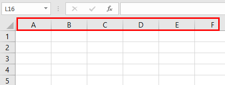
#3 – Column Header
As you can see, each column has its heading with alphabet characters representing each column separately.
Alphabets represent column headers, and similarly, row headersExcel Row Header is the grey column on the left side of column 1 in the worksheet that contains the numbers (1, 2, 3, etc.). To hide or reveal row and column headers, press ALT + W + V + H.read more are represented by numbers starting from 1. In recent versions of Excel, we have more than 1 million rows.

#5 – Spreadsheet Area
It is where we do the work. As you can see in the above overview image, we have small rectangular boxes, which are plenty. The combination of column and row forms a cell, a rectangular box. Each cell was identified by a unique cell address consisting of a column header followed by a row header. For example, the column header is A for the first cell, and the row header is 1, so the first cell address is A1.

It is the general overview of the Excel spreadsheet. Now, we will see how to work with this spreadsheet.
How to Work with Excel Spreadsheet?
Let us look at the example given below.
- To work with a spreadsheet, first, we need to select the cell we are looking to work with. For example, if we want the word Name in cell A1, select the cell and type Name in the cell.

- Then, select cell B1 and type Price.

- Now, we must return to cell A2 and type some fruit names.

- In the associated column, we must insert the price of each fruit.


It is the simple table we have created with Excel.
Steps to Format Excel Spreadsheet
It looks like raw data, but we can make this look beautiful by applying some excel formattingFormatting is a useful feature in Excel that allows you to change the appearance of the data in a worksheet. Formatting can be done in a variety of ways. For example, we can use the styles and format tab on the home tab to change the font of a cell or a table.read more, we can make this look beautiful.
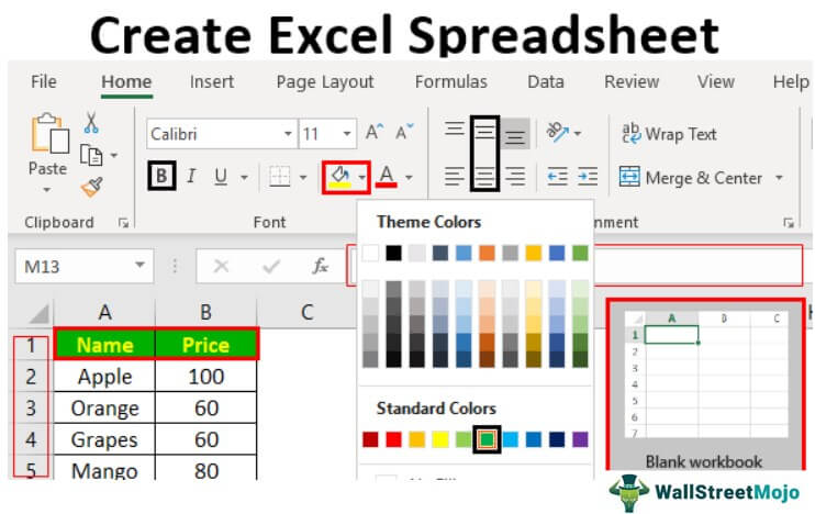
Step #1
We must first select the header and make the font “Bold.” The excel shortcut keyAn Excel shortcut is a technique of performing a manual task in a quicker way.read more to apply bold formatting is “Ctrl + B.”.

Step #2
Then, make the “Center” alignment.

Step #3
Now, fill in the background color for the selected cells.

Step #4
Change the font color to white.

Step #5
Now, apply borders to the data. Select the whole data range to use borders.
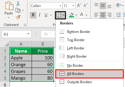
Now, the data looks organized. Like this, we can create a spreadsheet and work with it.
It is the basic level introduction to an Excel spreadsheet. Excel has a wide variety of tools to work with. We will see each tool explanation in separate dedicated articles that expose you to the advanced features.
Recommended Articles
This article is a guide to Creating an Excel Spreadsheet. We showed you how to create a spreadsheet through Excel, general overview tools available, examples, and a downloadable Excel template. You may learn more about Excel from the following articles: –
- Family Tree in Excel
- Word Cloud in Excel
- Basic Formulas in Excel
Create a Spreadsheet in Excel (Table of Content)
- Introduction to Create Spreadsheet in Excel
- How to Create a Spreadsheet in Excel?
Introduction to Create Spreadsheet in Excel
A spreadsheet is a grid-based file designed to manage or perform any calculation on personal or business data. It is the best choice for users because it has 400+ functions and features such as pivot, coloring, graph, chart, and conditional formatting. It is accessible in both Office 365 and MS Office. Office 365 is a cloud-based application, whereas MS Office is an on-premises solution.
The workbook is the Excel lingo for ‘spreadsheet.’ MS Excel uses this term to emphasize that a single workbook can contain multiple worksheets, each with its own data grid, chart, or graph.
How to Create a Spreadsheet in Excel?
Here are a few examples of creating different types of spreadsheets in Excel with the key features of the created spreadsheets.
You can download this Create Spreadsheet Excel Template here – Create Spreadsheet Excel Template
Example #1 – How to Create Spreadsheet in Excel?
Step 1: Open MS Excel.
Step 2: Go to Menu and select New >> Click on the Blank workbook to create a simple worksheet.
OR – Press Ctrl + N: To create a new spreadsheet.
Step 3: By default, Sheet 1 will be created as a worksheet in the spreadsheet. The name of the spreadsheet will be given as Book 1 if you are opening it for the first time.
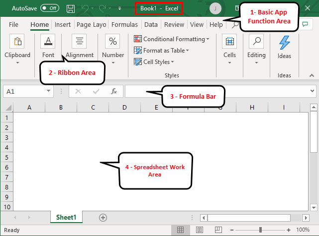
Key Features of the Created Spreadsheet:
- Basic App Functions Area: There is a green banner that contains all types of actions to perform on the worksheet, like – save the file, back or front step move, new, undo, redo, and many more.
- Ribbon Area: This is a gray area just below the basic app functions area called Ribbon. It contains data manipulation, a data visualizing toolbar, page layout tools, and many more.
- Spreadsheet Work Area: By default, a grid contains alphabetic columns like A, B, C, …, Z, ZA…, ZZ, ZZA… and rows as numbers like 1,2 3, …. 100, 101, and… so on. Each rectangle box in the spreadsheet is called a cell, like the one selected in the above image (cell A1). It is a cell where the user can perform their calculation for personal or business data.
- Formula Bar: It shows the data in the selected cell; if it contains any formula, it will show here. Like the above area, a search bar is available in the top right corner, and a sheet tab is available on the downside of the worksheet. A user can change the name of the sheet name.
Once you create an Excel Spreadsheet, you can convert it to a universally accepted format like PDF. For convenience, some useful Excel to PDF converters converts Excel to PDF files for free while maintaining the original formatting.
Example #2 – How to Create a Simple Budget Spreadsheet in Excel?
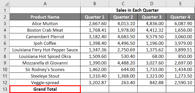
Suppose a user wishes to design a spreadsheet for budget calculation. For 2018, he has a few products and their quarterly sales. He now wants to present his client with this budget.
Let’s see how we can do this with the help of the spreadsheet.
Step 1: Open MS Excel.
Step 2: Go to Menu and select New >> Click on the Blank workbook to create a simple worksheet.
OR – Press Ctrl + N: To create a new spreadsheet.

Step 3: Go to the spreadsheet work area, sheet 1.
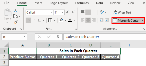
Step 4: Now create headers for Sales in each quarter in the first row by merging cells from B1 to E1. In row 2, give the product name and each quarter’s name.
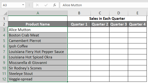
Step 5: Write down all product names in column A.
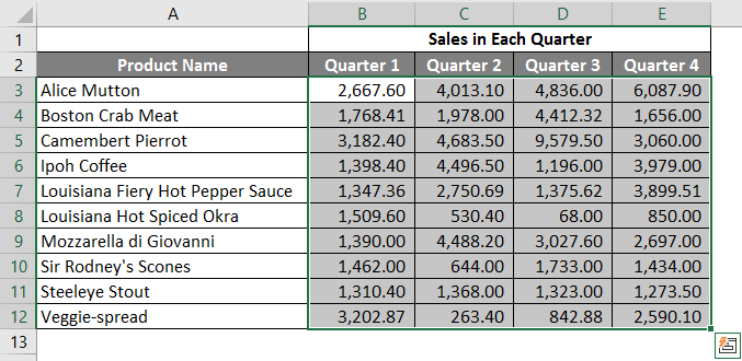
Step 6: Provide the sales data for each quarter before every product.
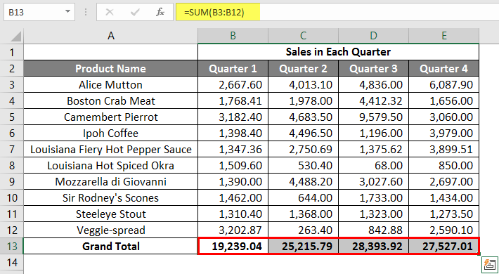
Step 7: In the next row, put one header for Grand Total and calculate each quarter’s total sales.
Step 8: Calculate the grand total for each quarter by summation >> apply in other cells in B13 to E13.
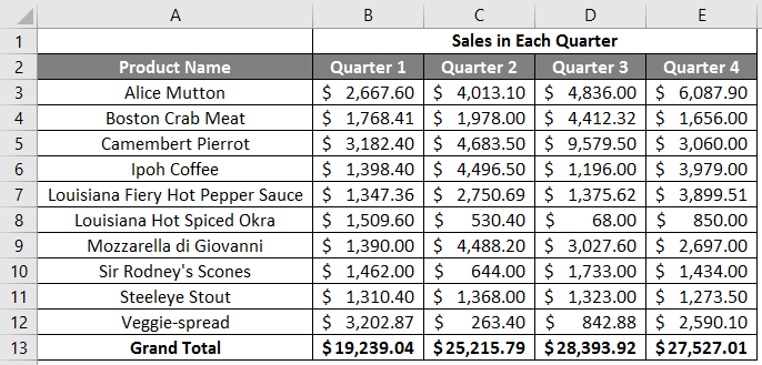
Step 9: Let’s convert the sales value into the ($) currency symbol.
Step 10: Create a Result Table with each quarter’s total sales.
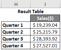
Plot the pie chart to represent the data to the client in a professional way that looks attractive. A user can change the look of the graph by just clicking on it.
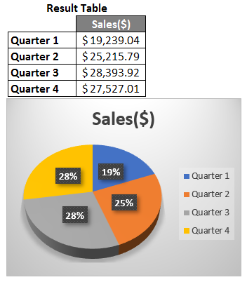
Summary of Example 2: As the user wants to create a spreadsheet to represent sales data to the client, it is done here.
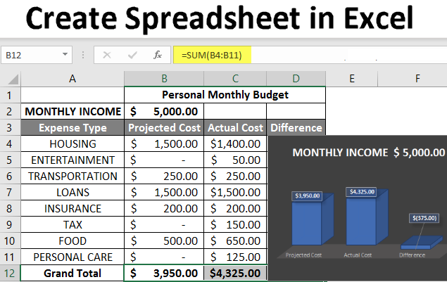
Example #3 – How to Create a Personal Monthly Budget Spreadsheet in Excel?
Let’s assume a user wants to create a spreadsheet to determine their monthly personal budget. For the year 2022, he has estimated costs and actual costs. He now wants to show his family this budget.
Let’s see how we can do this with the help of the spreadsheet.
Step 1: Open MS Excel.
Step 2: Go to Menu and select New >> Click on the Blank workbook to create a simple worksheet.
OR – Press Ctrl + N: To create a new spreadsheet.

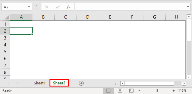
Step 3: Go to the spreadsheet work area, Sheet 2.
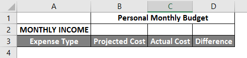
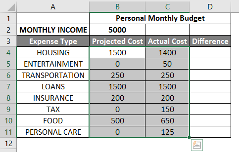
Step 4: Now create headers for Personal Monthly Budget in the first row by merging cells from B1 to D1. In row 2, give MONTHLY INCOME; in row 3, give Expense type, Projected Cost, Actual Cost, and Difference.
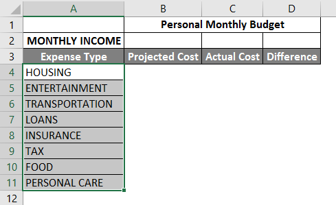
Step 5: Write down all the expenses in column A.
Step 6: Now, provide the monthly income, Projected cost, and Actual Cost data for each expense type.
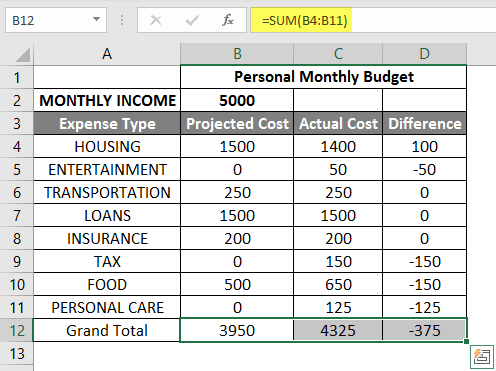
Step 7: In the next row, put one header for Grand Total and calculate the total and difference from the project to the actual cost.
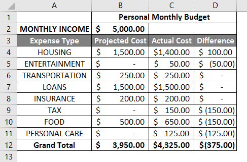
Step 8: Now highlight the header and add boundaries using toolbar graphics. >> The cost and income value in $, so make it by currency symbol.
Step 9: Create a Result Table with each quarter’s total sales.
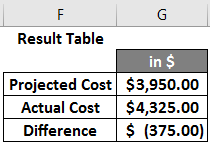
Step 10: Plot the pie chart to represent the data for the family. A user can choose one which he likes.
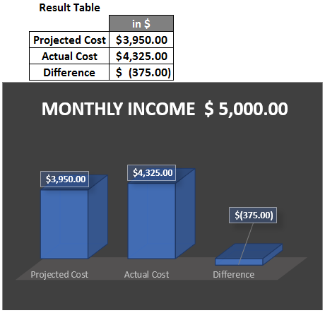
Summary of Example 3: As the user wanted to create a spreadsheet to represent monthly budget data to the family, we have created the same here. The close bracket shows in the data for the negative value.
Things to Remember
- A spreadsheet is a grid-based file designed to manage or perform any calculation on personal or business data.
- It is available in MS Office as well as Office 365.
- The workbook is the Excel lingo for ‘spreadsheet.’ MS Excel uses this term to emphasize that a single workbook can contain multiple worksheets.
How to add data in a spreadsheet Video
Recommended Articles
This article is a comprehensive guide to creating Spreadsheets in Excel. Here we have discussed how to create a Spreadsheet in Excel, examples, and a downloadable Excel template. You may also look at the following articles to learn more –
- Excel Spreadsheet Formulas
- Group Worksheets In Excel
- Excel Spreadsheet Examples
- Worksheets in Excel
Updated: 03/12/2022 by
In Microsoft Excel, you can add one or more worksheets to a workbook file. You can also rename, copy, move, and delete a worksheet. To perform any of these actions, follow the steps on this page.
How to add a new worksheet
To add a new worksheet to your Excel file, follow the steps below for the version of Excel on your computer.
Excel 2013 and later
- At the bottom of the Excel window, to the right of the last worksheet listed, click the + symbol.
- A new worksheet is created, with a default name of «Sheet» plus a number. The number used is one more than the number of existing worksheets. For example, if there are three worksheets in the Excel file, the new worksheet is named «Sheet4».
Tip
You can also use the keyboard shortcut Alt+Shift+F1 to create a new worksheet tab in Excel.
Excel 2010 and earlier
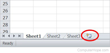
- At the bottom of the Excel window, to the right of the last worksheet listed, click the small tab with a folder-like icon.
- A new worksheet is created, with a default name of «Sheet» plus a number. The number used is one more than the number of existing worksheets. For example, if there are three worksheets in the Excel file, the new worksheet is named «Sheet4».
How to rename a worksheet
To rename a worksheet in an Excel file, follow the steps below.
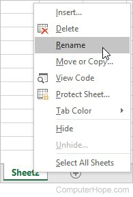
- At the bottom of the Excel window, right-click the worksheet tab you want to rename.
- Click the Rename option.
- Type in the new name for the worksheet and press Enter.
Note
There is a 31 character limit for a worksheet name.
How to copy a worksheet
To copy a worksheet, copying all contents of that worksheet to a new worksheet, follow the steps below.
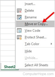
- At the bottom of the Excel window, right-click the worksheet tab you want to copy.
- Click the Move or Copy option.
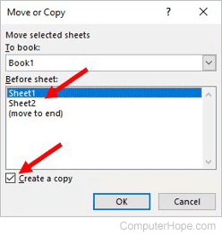
- In the Move or Copy window, in the Before sheet section, select the worksheet where you want to place the copied worksheet.
- Check the box for the Create a copy option, then click OK.
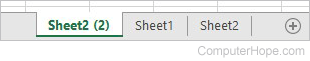
A copy of the worksheet is added and placed before the worksheet you selected in step 3 above. For example, if you had two worksheets named «Sheet1» and «Sheet2,» and you selected Sheet2 in step 3, a copy of Sheet2 would be placed before the Sheet1. The result would look like the example picture below. The worksheet named «Sheet2 (2)» is the copy of Sheet2.
- For additional details about how to copy worksheets and workbooks, see: How to copy an entire worksheet in Excel.
How to move or change the order of worksheets
If you want to change the order or move worksheets in your workbook, click-and-drag any worksheet into the order you want it placed. For example, to make the first tab the last tab, click it, and while continuing to hold the button down, drag it after the far-right tab.
How to delete a worksheet from a workbook
- In the sheet tab listing, right-click the worksheet you want to delete.
- From the right-click menu that appears, click the Delete option.