
Create and format tables
Create and format a table to visually group and analyze data.
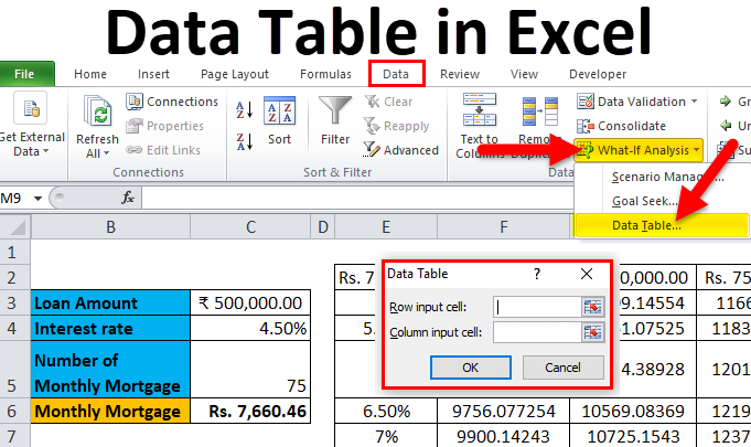
Note: Excel tables shouldn’t be confused with the data tables that are part of a suite of What-If Analysis commands (Forecast, on the Data tab). See Introduction to What-If Analysis for more information.

Try it!
-
Select a cell within your data.
-
Select Home > Format as Table.
-
Choose a style for your table.
-
In the Create Table dialog box, set your cell range.
-
Mark if your table has headers.
-
Select OK.
-
Insert a table in your spreadsheet. See Overview of Excel tables for more information.
-
Select a cell within your data.
-
Select Home > Format as Table.
-
Choose a style for your table.
-
In the Create Table dialog box, set your cell range.
-
Mark if your table has headers.
-
Select OK.
To add a blank table, select the cells you want included in the table and click Insert > Table.
To format existing data as a table by using the default table style, do this:
-
Select the cells containing the data.
-
Click Home > Table > Format as Table.
-
If you don’t check the My table has headers box, Excel for the web adds headers with default names like Column1 and Column2 above the data. To rename a default header, double-click it and type a new name.
Note: You can’t change the default table formatting in Excel for the web.
Want more?
Overview of Excel tables
Video: Create and format an Excel table
Total the data in an Excel table
Format an Excel table
Resize a table by adding or removing rows and columns
Filter data in a range or table
Convert a table to a range
Using structured references with Excel tables
Excel table compatibility issues
Export an Excel table to SharePoint
Need more help?
One Variable Data Table | Two Variable Data Table
Instead of creating different scenarios, you can create a data table to quickly try out different values for formulas. You can create a one variable data table or a two variable data table.
Assume you own a book store and have 100 books in storage. You sell a certain % for the highest price of $50 and a certain % for the lower price of $20. If you sell 60% for the highest price, cell D10 below calculates a total profit of 60 * $50 + 40 * $20 = $3800.
One Variable Data Table
To create a one variable data table, execute the following steps.
1. Select cell B12 and type =D10 (refer to the total profit cell).
2. Type the different percentages in column A.
3. Select the range A12:B17.
We are going to calculate the total profit if you sell 60% for the highest price, 70% for the highest price, etc.

4. On the Data tab, in the Forecast group, click What-If Analysis.

5. Click Data Table.

6. Click in the ‘Column input cell’ box (the percentages are in a column) and select cell C4.
We select cell C4 because the percentages refer to cell C4 (% sold for the highest price). Together with the formula in cell B12, Excel now knows that it should replace cell C4 with 60% to calculate the total profit, replace cell C4 with 70% to calculate the total profit, etc.

Note: this is a one variable data table so we leave the Row input cell blank.
7. Click OK.
Result.

Conclusion: if you sell 60% for the highest price, you obtain a total profit of $3800, if you sell 70% for the highest price, you obtain a total profit of $4100, etc.
Note: the formula bar indicates that the cells contain an array formula. Therefore, you cannot delete a single result. To delete the results, select the range B13:B17 and press Delete.
Two Variable Data Table
To create a two variable data table, execute the following steps.
1. Select cell A12 and type =D10 (refer to the total profit cell).
2. Type the different unit profits (highest price) in row 12.
3. Type the different percentages in column A.
4. Select the range A12:D17.
We are going to calculate the total profit for the different combinations of ‘unit profit (highest price)’ and ‘% sold for the highest price’.

5. On the Data tab, in the Forecast group, click What-If Analysis.
6. Click Data Table.
7. Click in the ‘Row input cell’ box (the unit profits are in a row) and select cell D7.
8. Click in the ‘Column input cell’ box (the percentages are in a column) and select cell C4.
We select cell D7 because the unit profits refer to cell D7. We select cell C4 because the percentages refer to cell C4. Together with the formula in cell A12, Excel now knows that it should replace cell D7 with $50 and cell C4 with 60% to calculate the total profit, replace cell D7 with $50 and cell C4 with 70% to calculate the total profit, etc.

9. Click OK.
Result.

Conclusion: if you sell 60% for the highest price, at a unit profit of $50, you obtain a total profit of $3800, if you sell 80% for the highest price, at a unit profit of $60, you obtain a total profit of $5200, etc.
Note: the formula bar indicates that the cells contain an array formula. Therefore, you cannot delete a single result. To delete the results, select the range B13:D17 and press Delete.
Data Table in Excel (Table of Contents)
- Data Table in Excel
- How to Create Data Table in Excel?
Data Table in Excel
Data tables are used to analyze the changes seen in your final result when certain variables are changed from your function or formula. Data tables are one of the existing parts of What-If analysis tools, which allow you to observe your result by experimenting it with different values of variables and to compare the outcomes stored by the data table.
There are two types of a data table, which are as follows:
- One-Variable Data Table.
- Two-Variable Data Table.
How to Create Data Table in Excel?
Data Table in Excel is very simple and easy to create. Let’s understand the working of the Data Table in Excel by Some Examples.
You can download this Data Table Excel Template here – Data Table Excel Template
Data Table in Excel Example #1 – One-Variable Data Table
One-variable data tables are efficient in the case of analyzing the changes in the result of your formula when you change the values for a single input variable.
Use case of One-Variable Data Table in Excel:
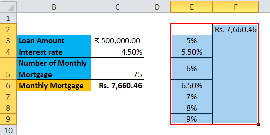
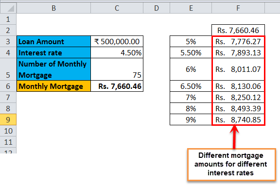
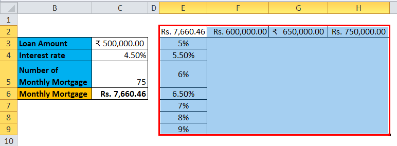
The one-variable data table is useful in scenarios where a person can observe how different interest rates change the amount of their mortgage amount to be paid. Consider the below figure, which shows the mortgage amount calculated based on the interest rate using the PMT function.
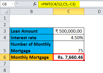
The table above shows the data where the mortgage amount is calculated based on the interest rate, mortgage period and loan amount. It uses the PMT formula to calculate the monthly mortgage amount, which can be written as =PMT (C4/12, C5,-C3).
In the case of observing the monthly mortgage amount for different interest rates, where the interest rate is considered as a variable. In order to do this, there is a need for creating a one-variable data table. The steps to create the one-variable data table are as follows:
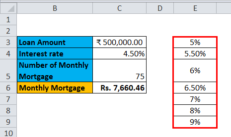
Step 1: Prepare a column which consists of different values for the interest rates. We have entered different values for interest rates in the column which is highlighted in the figure.
Step 2: In the cell (F2), which is one row above and diagonal to the column which you prepared in the previous step, type this = C6.
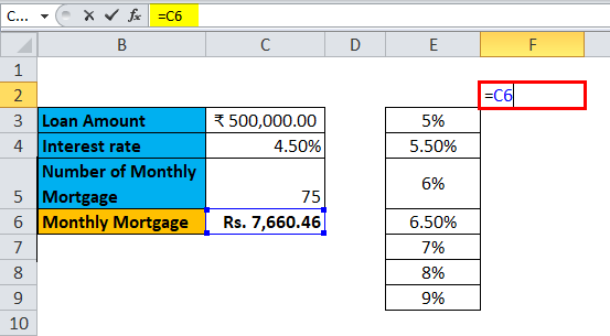
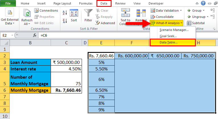
Step 3: Select the entire prepared column by values of different interest rates along with the cell where you had inserted the value, i.e. F2 cell.
Step 4: Click on the ‘Data’ tab and select ‘What-If Analysis’, and from the options popped down, select ‘Data Table’.
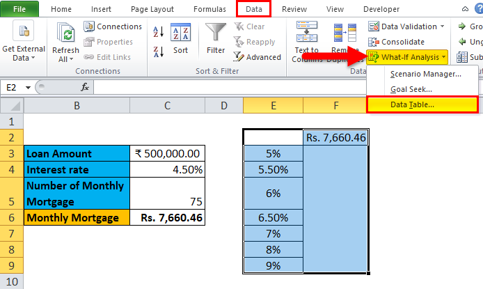
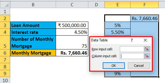
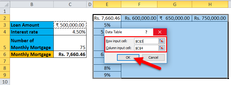
Step 5: Data table dialog box will appear.
Step 6: In the Column input cell, refer to cell C4 and click OK.
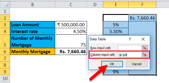
In the dialog box, we refer to the cell C4 in the Column input cell and keep the row input cell empty as we are preparing a data table with one variable.
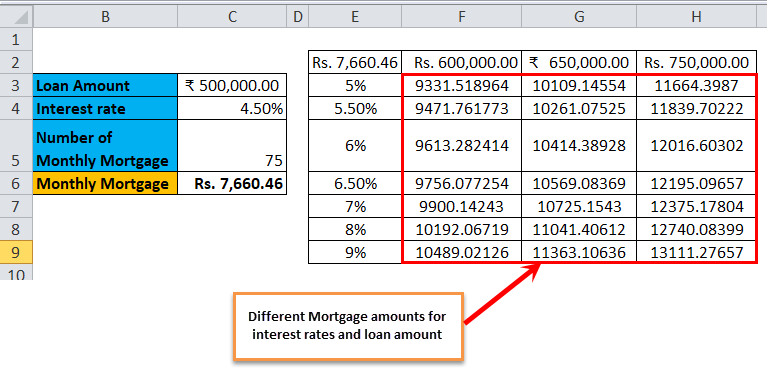
Step 7: After following all the steps, we get all the different mortgage amounts for all entered interests rates in column E (unmarked), and the different mortgage amounts are observed in column F (marked).
Data Table in Excel Example #2 – Two-Variable Data Table
Two-variable data tables are useful in scenarios where a user needs to observe the changes in the result of their formula when they change two input variables simultaneously.
Use-case of Two-Variable Data Table in Excel:
The two-variable data table is useful in scenarios where a person can observe how different interest rates and loan amounts change the amount of their mortgage amount to be paid. Instead of calculating for individual values separately, we can observe them with instantaneous results. Consider the below figure, which shows the mortgage amount calculated based on the interest rate using the PMT function.
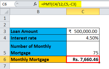
The above example is similar to our example shown in the previous case for a one-variable data table. Here the mortgage amount in cell C6 is calculated based on the interest rate, mortgage period and loan amount. It uses the PMT formula to calculate the monthly mortgage amount, which can be written as =PMT (C4/12, C5,-C3).
In order to explain the two-variable data table with reference to the above example, we will show the different mortgage amounts and choose the best which suits you by observing the different values of interest rates and loan amount. In order to do this, there is a need for creating a two-variable data table. The steps to create the one-variable data table are as follows:
Step 1: Prepare a column which consists of different values for the interest rates and loan amount.
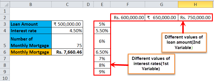
We have prepared a column consisting of the different interest rates, and in the cell diagonal to starting cell of the column, we have entered the different values of the loan amount.
Step 2: In the cell (E2), which is one row above to the column which you prepared in the previous step, type this = C6.
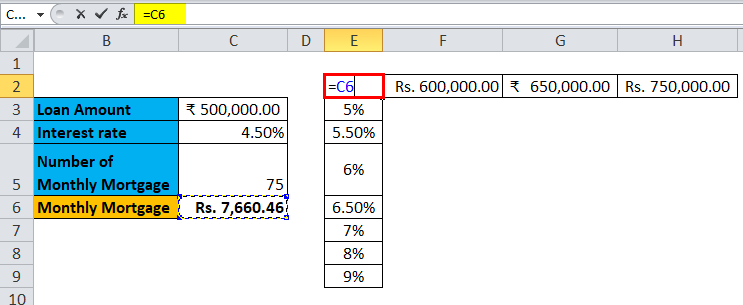
Step 3: Select the entire prepared column by values of different interest rates along with the cell where you had inserted the value, i.e. E2 cell.
Step 4: Click on the ‘Data’ tab and select ‘What-If Analysis’, and from the options popped down, select ‘Data Table’.
Step 5: A Data table dialog box will appear. The ‘Column input cell’ refers to cell C4 and in the ‘Row input cell’ C3. Both the values are selected as we are changing both the variables and Click OK.
Step 6: After following all the steps, we get different values of mortgage amounts for different values of interest rates and loan amount.
Things to Remember About Data Table in Excel
- For one variable data table, the ‘Row input cell’ is left empty, and in a two-variable data table, both ‘Row input cell’ and ‘Column input cell’ are filled.
- Once the What-If analysis is performed, and the values are calculated, you cannot change or modify any cell from the set of values.
Recommended Articles
This has been a guide to a Data Table in Excel. Here we discuss its types and how to create data table examples and downloadable excel templates. You may also look at these useful functions in excel –
- Two-Variable Data Table in Excel
- One Variable Data Table in Excel
- Excel Data Visualization
- Database Function in Excel
How to Make a Data Table in Excel: Step-by-Step Guide (2023)
Data tables in Excel are used to perform What-if Analysis on a given data set.
Using data tables, you can analyze the changes to the output value by changing the input values to a formula.
There is so much that you can do using data tables in Excel. 😀
Continue reading the article below to learn it all.
Also, download our sample workbook here to practice the examples given in this guide.
What is an Excel data table?
An Excel Data table is a What-if Analysis tool. It allows users to use different input values for a variable and assess the changes to the output value.

These are especially of help if you are operating a formula in Excel where the output depends on several variables. And you are keen to compare the results for different inputs to the formula.
Presently, Excel offers a one-variable and two-variable data table only. This means you can choose any two variable values (at max) from any formula to test.
Jump right into the article below to learn all about a data table in Excel. 🔔
How to create a one-variable data table in Excel
A one-variable data table in Excel allows users to test one variable.
For example, see the image below.

The image shows the particulars of a loan. We have three main variables in the data.
- The amount of loan
- The rate of interest/profit
- The tenure of the loan (until it is paid back)
Example 1: Column Input Cells
In this example, let’s see keep the interest rate as the variable.
What is the yearly payment to be made against the loan?
1. Write the PMT function to find the yearly repayment against the loan.
= PMT (B3, B4, B2)
= PMT (Interest Rate, Periods of Repayment, Amount of Loan Today)

2. Multiply this number by the number of payments to be made.

That’s the total amount to be paid against the loan over 5 years.
So how much is the interest on the loan?
3. Subtract the amount of loan from the amount of repayment.

Everything’s good and sorted.
Now, what if you want to see how the repayments change if one variable (the interest rate) changes?
Do not re-perform the entire calculation all over again. The Data Table (What-if analysis) will do it for you.
4. List down the variable (interest rate in this case) that is to be changed.

5. Create a link by referring to the targeted output for each interest rate in the corresponding column.
We want Excel to give us the repayments for different interest rates. So, we have created a link to the repayment in the original calculation.

6. Select the Inputs table (the interest rates and the corresponding column for targeted output).

7. Go to Data Tab > Forecast > What-If Analysis Tools > Data Table.

This will take you to the Data Table dialog box.
8. In the Column Input Cell box, create a reference to the ‘Interest Rate’ from the original table.

Reference is made to the Interest rate because that is the variable in our data. We want to experiment with how the changing interest rates affect repayments.
We have created a reference in the Column Input Cell box and not the Row Input Cell box. This is because our Input data is in the form of a column and not a row.
9. All set. Hit Okay and Ta-da! 😃

Excel creates a one-variable data table to calculate the repayments for different interest rates.
Example 2: Row Input Cells
Let’s bring a slight variation to the above data. This time the one variable of the data is the amount of the loan.
Also, let’s change the shape of Input Data from a Column to a Row.

1. Select the Inputs Data.

2. Go to Data Tab > Forecast > What-If Analysis Tools > Data Table.
3. In the ‘Data Table’ dialog box, create a reference to the Loan amount in the Row Input Cell box.

This time the variable is the amount of the loan. We want to experiment with how the changing loan amount affects the repayments.
Must note that we have created a reference to the ‘Row Input Cell’ this time. This is because our Input Data is row-oriented.
4. Click ‘Okay’ to see the repayment amount for differing amounts of loans.

What if we want to see how the total interest changes by the change in the loan amount?
Simple, refer to the amount of interest in the Inputs Data.

And there it is! Excel shows the changes to total interest instead of repayments.

How to create multiple one-variable data tables?
In the above example, what if you want to see the change in interest rates on both the repayments and total interest?
Create multiple Excel data tables. Simple.
1. In the Input Data, make two columns next to the variable interest rates.
2. In the first column, create a reference to the repayment calculation in the original data.

3. In the second column, create a reference to the total interest in the original data.

4. Create a one-variable data table by referring to the interest rate in the Column Input Cell box.

5. Click Okay, and there you go! 🙂

Excel shows the result of changes in interest rates on repayments and loan amounts.
How to make a two-variable data table in Excel?
The two-variable data table is more of a two-dimensional table. It allows you to analyze how your final output changes from the changes in any two variables of your data.
Let’s continue the example above to create a two-variable data table in Excel.
This time, let’s select two variables from the data, Interest Rate, and Loan Amount. We want to see how the repayments change when both these variables change.
1. Create a two-dimensional data table with each variable on one side of the table.

In the above image, we have set the interest rates in a columnar format. Whereas the loan amount takes the shape of a row.
2. Select the intersecting cell of both the data sides.
3. In this cell, create a reference to the calculation of the repayment in the original table.

This is because we want to see how the repayments change with changes in the interest rate and the loan amount.
Our Input Data is now ready. Let’s now create a data table and perform the What-if Analysis.
4. Select the entire Data Table.
5. Go to Data Tab > Forecast > Click What-if Analysis Tools > Data table.

6. This opens up the data table dialog box.
7. Against the Column Input Cell box, create a reference to the interest rate from the source data.

Pay attention to how a reference is created to the interest rate against the Column Input Cell. This is because the possible input values for interest rate (the first variable) are in the shape of a column.
8. Against the ‘Row Input Cell’, create a reference to the amount of loan from the source data.

The Row Input Cell refers to the amount of the loan. This is because possible input values for the loan (second variable) are in the shape of a row.
9. Click ‘Okay’, and you’re good to go.

Woah! This seems like a very densely packed data table.
What is this? See below.

Each cell of this data table is mutual to two cells. For example, in the image above, the highlighted cell shows the amount of repayment, if the interest rate changes to 12% and the loan amount changes to 2000.
Must Note: A two-variable data table is a two-dimensional table. It captures the result of the change in any two variables at the same time.
The data table formula above is an array formula. To double-check, click on any cell from the data table and see the formula bar.
You will find the formula enclosed in curly brackets. A formula enclosed in curly brackets is an Array formula.
Trouble Shooting the Two-Variable Data Table
The Two-Variable data table in Excel seems no less than magic. A heap of calculations is only a click away.
A two-variable data table is an array, and there is something you must know about a table array.
1. Editing a two-variable data table
Once you have created a two-variable data table, try clicking on any individual cell from the data table and making some changes to it.

You cannot make changes to a part of this data! This is all that Excel has to say in return.
A data table is an array, and you cannot make changes to individual cells of an array.
To make any changes to the data table, click the data table and select the whole of it.
1. From the formula bar, delete the Table formula.

2. Type in the desired value (let’s say 10) and hit Ctrl + Enter.
3. The entire table will be replaced by 10.

You can now make changes to any individual cells as it is no more an array.
2. Deleting a two-variable data table
Deleting two-variable data is a little science.
You cannot delete an individual value from the data table. However, you can only delete the whole data table.
- Select the entire array (whole data table).
- Press the delete key.
- And your data table is gone.
That’s it – Now what?
Data Tables can save you big on time.
In the article above, we have learned almost all about data tables in Excel – starting from creating a single-variable data table, and multiple single-variable data tables (in one go) to creating multiple-variable data tables.
And of course, many tips.
While data tables help data analysis in Excel, you’d need many other functions of Excel to handle big data sets in Excel. The most important of these include the VLOOKUP, SUMIF, and IF functions.
Learn each of these three functions by signing up for my free 30-minute email course that teaches you these functions (and more!).
Kasper Langmann2023-01-19T12:23:16+00:00
Page load link
Data Table is a tool present in Microsoft Excel as one of the three What-If Analysis tools namely Scenario Manager, Goal Seek, and Data Table. It is a tool, that allows one to try out various input values for the formulas present in their sheet and see how changes in those values affect the output in the cells. To apply a data table tool anywhere in the excel sheet, there must be a table and the formula whose values will be replaced by the row and column values must be kept in the top-left corner or the top-right corner of the table according to the variables used to replace the formula values. In this article, we will learn about data tables in excel.
Use of DataTable
Data tables can be used to replace the values of a formula present in the sheet with the values present in either the column or row of any table. With data tables, one can replace at most two values in the formula present in the sheet. For example, we can see in the below figures, there is an excel sheet that is used to calculate simple interest over a given amount for a given number of years for a given rate of interest per annum. With the help of a Data Table, we can calculate the interest for the same amount with different numbers of years and with different rates of interest. We can also, calculate the interest for different amounts, for different numbers of years for a fixed rate of interest very easily.
An excel sheet containing a table with a formula:


Types of Data Tables
One Variable Data Table
In a one-variable data table, only one of the formula values is replaced with the row or column values of a table of data.
For Example:
Let us say we want to find interest on the principal amount of the loan for 4 years for various interest rates, we can do this by placing the interest rates in either the row or column of a table and then using the data table we can replace the interest rate values with the row or column values, in the example below, we have placed the variables in the column of a table. The cell containing the formula is placed in the top right corner which contains empty cells for storing the calculated interest but do remember to keep the cells containing the other values in the formula linked with the cell containing the formula. The process is done as shown below:

Following are the steps:
Step 1: The top right cell is the cell that contains the formula for simple interest and it is linked with the cells containing the value of principal amount, number of years, and interest rate. The formula is =B3*B4*B5.

Step 2: To use the data table tool, we need to select the table with all the inputs and the cell containing the formula. Go to what-if analysis, and select Data Table. A Data-Table dialogue box appears. Add, Column Input cell value as $B$5. Click Ok.

Step 3: If the variable interest rates were kept in the rows then we would have done the same thing but instead of putting B5 in the column input, we would have placed it in the row input. Below, are shown the values of Interest in the excel sheet.

Two-Variable Data Table
In a two-variable data table, two of the formula values are replaced with the row and column values of a table of data. Two is the maximum number of values that can be used as variables in a data table since the values are replaced with row and column values which is a 2-D structure.
For Example:
Let us say we want to find interest on the principal amount of the loan for various numbers of years along with various interest rates, we can do this by placing the interest rates in either the row or column of a table and placing the numbers of years in the other row or column of the table mentioned before, then using the data table we can replace the interest rate values with the row or column values and numbers of years with the other row or column, in the example below we have placed the interest rate variables in the column and numbers of years variable in the row of a table. The cell containing the formula is placed in the top left corner. Do remember to keep the cells containing the principal amount in the formula linked with the cell containing the formula. The process is done as shown below:

Following are the steps:
Step 1: The top left cell is the cell that contains the formula for simple interest and it is linked with the cell containing the value of the principal amount. The formula is =B3*B4*B5.

Step 2: To use the data table tool, we need to select the table with all the inputs and the cell containing the formula. Go to what-if analysis, and select Data Table. A Data-Table dialogue box appears. Add, Column Input cell value as $B$5, and Row input cell value as $B$4. Click Ok.

Step 3: We can interchange the values in the rows and columns but accordingly we have to change the row and column input values in the data table. Below, are shown the values of interest for the various number of years.
