
Excel for Microsoft 365 Excel for Microsoft 365 for Mac Excel for the web Excel 2021 Excel 2021 for Mac Excel 2019 Excel 2019 for Mac Excel 2016 Excel 2016 for Mac Excel 2013 Excel 2010 Excel 2007 Excel for Mac 2011 Excel Starter 2010 More…Less
The COUNT function counts the number of cells that contain numbers, and counts numbers within the list of arguments. Use the COUNT function to get the number of entries in a number field that is in a range or array of numbers. For example, you can enter the following formula to count the numbers in the range A1:A20: =COUNT(A1:A20). In this example, if five of the cells in the range contain numbers, the result is 5.

Syntax
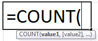
COUNT(value1, [value2], …)
The COUNT function syntax has the following arguments:
-
value1 Required. The first item, cell reference, or range within which you want to count numbers.
-
value2, … Optional. Up to 255 additional items, cell references, or ranges within which you want to count numbers.
Note: The arguments can contain or refer to a variety of different types of data, but only numbers are counted.
Remarks
-
Arguments that are numbers, dates, or a text representation of numbers (for example, a number enclosed in quotation marks, such as «1») are counted.
-
Logical values and text representations of numbers that you type directly into the list of arguments are counted.
-
Arguments that are error values or text that cannot be translated into numbers are not counted.
-
If an argument is an array or reference, only numbers in that array or reference are counted. Empty cells, logical values, text, or error values in the array or reference are not counted.
-
If you want to count logical values, text, or error values, use the COUNTA function.
-
If you want to count only numbers that meet certain criteria, use the COUNTIF function or the COUNTIFS function.
Example
Copy the example data in the following table, and paste it in cell A1 of a new Excel worksheet. For formulas to show results, select them, press F2, and then press Enter. If you need to, you can adjust the column widths to see all the data.
|
Data |
||
|
12/8/08 |
||
|
19 |
||
|
22.24 |
||
|
TRUE |
||
|
#DIV/0! |
||
|
Formula |
Description |
Result |
|
=COUNT(A2:A7) |
Counts the number of cells that contain numbers in cells A2 through A7. |
3 |
|
=COUNT(A5:A7) |
Counts the number of cells that contain numbers in cells A5 through A7. |
2 |
|
=COUNT(A2:A7,2) |
Counts the number of cells that contain numbers in cells A2 through A7, and the value 2 |
4 |
Need more help?
What Is COUNT In Excel?
The COUNT function in Excel counts the number of cells containing numerical values within the given range. It always returns an integer value.
The COUNT in Excel is an inbuilt statistical function, so we can insert the formula from the “Function Library” or enter it directly in the worksheet.
For example, to count a range of cells that contain a date before April 1, 2021, the formula used is “=COUNT(“Cell Range”, “<”&DATE (2021,4,1))”. The date is entered by using the DATE functionThe date function in excel is a date and time function representing the number provided as arguments in a date and time code. The result displayed is in date format, but the arguments are supplied as integers.read more.
Table of contents
- What Is COUNT In Excel?
- Syntax Of COUNT Excel Formula
- How To Use COUNT Function In Excel?
- Examples
- The Characteristics Of The COUNT Function
- Important Things To Note
- Frequently Asked Questions (FAQs)
- COUNT Function In Excel Video
- Download Template
- Recommended Articles
- In a given dataset, the COUNT function in Excel returns the count of the numeric values.
- It counts only the numbers and not the logical values, empty cells, text, or error values when the argument seems to be an array or reference.
- The usage of the COUNT and VBA (VBA Excel COUNT) functions are the same in Excel.
- The COUNTA function is a further extension of the COUNT function. It counts logical values, text, or error values. The COUNTIF function (another extension of the COUNT function) counts the numbers that meet a specified criterion.
Syntax Of COUNT Excel Formula
The syntax of the COUNT Excel formula is,
The arguments of the COUNT Excel formula are,
- value1, [value2], …, [value n]: It is a mandatory argument. It can range up to 255 values. The value can be a cell referenceCell reference in excel is referring the other cells to a cell to use its values or properties. For instance, if we have data in cell A2 and want to use that in cell A1, use =A2 in cell A1, and this will copy the A2 value in A1.read more or a range of values. It is a collection of worksheet cells containing a variety of data, out of which only the cells containing numbers are counted.
How To Use COUNT Function In Excel?
We can use the COUNT Excel function in 2 ways, namely:
- Access from the Excel ribbon.
- Enter in the worksheet manually.
Method #1 – Access from the Excel ribbon
Choose an empty cell for the result → select the “Formulas” tab → go to the “Function Library” group → click the “More Functions” option drop-down → click the “Statistical” option right arrow → select the “COUNT” function, as shown below.

The “Function Arguments” windowappears. Enter the arguments in the “Value1”, “Value2”, etc. fields, and click “OK”, as shown below.

Method #2 – Enter in the worksheet manually
- Select an empty cell for the output.
- Type =COUNT( in the selected cell. [Alternatively, type =C or =COU and double-click the COUNT function from the list of suggestions shown by Excel.
- Enter the argument as cell value or cell reference and close the brackets.
- Press the “Enter” key.
Basic Example – Count Numbers in the Given Range
Let us look at an example to apply the COUNT function to Count Numbers in the Given Range. (shown in the table below).
Select cell B10, enter the formula =COUNT(B3:B8), and press “Enter”.
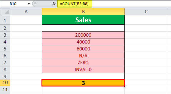
The output is shown above. The range B3:B8 contains only three numeric values. Hence, the COUNT function returns 3.
Examples
We will consider some scenarios using COUNT Function in Excel examples. Each example covers a different case, implemented using the COUNT function.
Example #1 – Count Non-empty Cells
Let us apply the COUNTA functionThe COUNTA function is an inbuilt statistical excel function that counts the number of non-blank cells (not empty) in a cell range or the cell reference. For example, cells A1 and A3 contain values but, cell A2 is empty. The formula “=COUNTA(A1,A2,A3)” returns 2.
read more to the range of cells A1:A5 provided in the below table to find the count of the number of cells that are not empty.
Select cell B1, enter the formula =COUNTA(A1:A5), and press “Enter”.

The output is shown above. The COUNTA function counts the number of cells from A1 through A5 that contain some data. It returns the value as 4, as cells A1, A2, A3, and A4 are not empty, and only cell A5 is empty.
Example #2 – Count the Number of Valid Dates
Let us apply the COUNT function to count the number of valid dates to the range of cells C3:C8 (shown in the table below).
Select cell C10, enter the formula =COUNT(C3:C8), and press “Enter”.
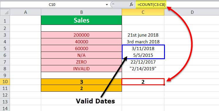
The output is shown above. The range contains dates in different formats. Out of this, only two dates are valid. Hence, the formula returns 2.
Example #3 – Multiple Parameters
Let us apply the COUNT formula to the range of excel cells C3:C7 (provided in the table below) along with another parameter that is hard-coded with a value of 5.
Select cell C11, enter the formula =COUNTA(C3:C7,5), and press “Enter”.
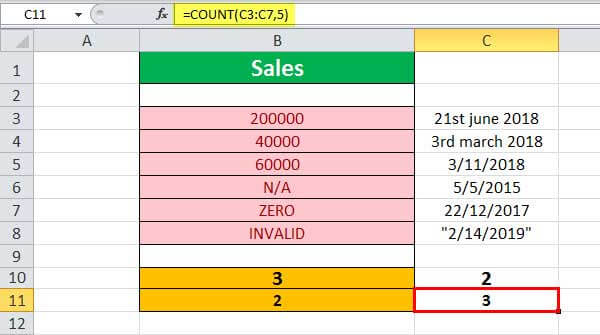
The output is shown above. The number of cells (C3 through C7) with valid numeric values or dates is 2, plus 1 for the number 5. Hence the COUNT formula returns the result as 3 (cells C5, C6, and the number 5). Note that the date in cell C7 is invalid, and so is not taken into account in the given results.
Example #4 – Invalid Numbers
Let us apply the COUNT formula to the range of values B6:B8 (shown in the table below) containing invalid numbers.
Select cell B12, enter the formula =COUNTA(B6:B8), and press “Enter”.
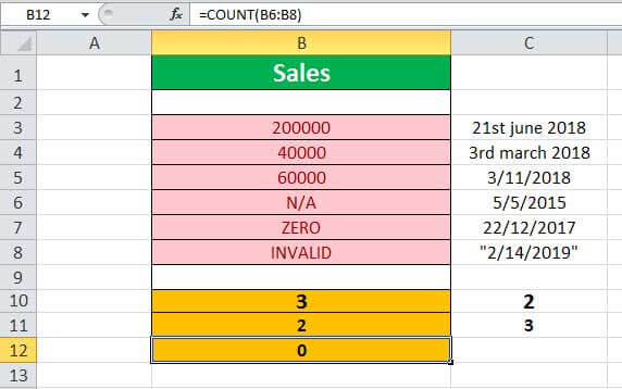
The output is shown above. The range does not have any valid number. Hence, the result returned by the formula is 0, indicated in cell B12.
Example #5 – Empty Range
Let us apply the COUNT function to the range of values in cells D3:D5, which is an empty range.
Select cell D10, enter the formula =COUNTA(D3:D5), and press “Enter”.

The output is shown above. The given range does not have any numbers, and it is empty. Hence, the result returned by the formula is 0, indicated in cell D10.
The Characteristics Of The COUNT Function
The features of the COUNT Excel function are listed as follows:
- It counts the list of parameters containing the logical values and text representations.
- It does not count the error values or text which cannot be converted into numbers.
- It counts only the numbers and not the logical values, empty cells, text, or error values when the argument seems to be an array or reference.
- A further extension to the COUNT function is the COUNTA function. It counts logical values, text, or error values.
- Another extension of the COUNT function is the COUNTIF function, which counts the numbers that meet a specified criterion.
Important Things To Note
- Since the COUNT function has other related functions such as COUNTA, COUNTIF, COUNTBLANK, etc., we must ensure we enter the right function name to avoid getting a “#NAME?” error.
- In a selected cell range, the function ignores the blank cells, non-numeric cells, etc.
Frequently Asked Questions (FAQs)
1. How to use the Excel COUNT function?
The COUNT function provides the count of cells containing numbers within the given range of cells. It also counts numeric values within the list of arguments.
The formula of the COUNT in excel is =COUNT(value 1, [value 2],……, and so on).
2. What is the COUNTIF formula?
The COUNTIF function counts cells in a range that meets a single criterion. It counts cells that contain dates, numbers, and text.
The COUNTIF formula in excel is =COUNTIF(range, condition)
Here, the range is a series of cells to count.
3. What is the difference between the COUNT and COUNTA functions in Excel?
The COUNT function is generally used to count a range of cells containing numbers or dates. It excludes blank cells. And the COUNTA function, whichstands for count all, will count the numbers, dates, text, or a range containing a mixture of all these items. It does not count blank cells.
COUNT Function In Excel Video
Download Template
This article must help understand the COUNT function in Excel with its formulas and examples. You can download the template here to use it instantly.
You can download this COUNT Formula Excel Template here – COUNT Formula Excel Template
Recommended Articles
This is a guide to the COUNT Function in Excel. Here, we count number of cells with numeric values, COUNTA, COUNTIF, examples & a downloadable template. You may also look at the below useful functions in Excel –
- Example of COUNTIF with Multiple Criteria
- INT Function in Excel (Integer)INT or integer function in excel returns the nearest integer of a given number and is used when we have many data sets and each data in a different format.read more
- AVERAGE Function in Excel
For getting the count of numbers, dates, text, empty or non-blank cells, you may use various built-in functions in Excel.
Depending on the requirement, you may choose which one to use; for example, if you require the count of cells that contain numbers only, you may use the Excel COUNT function.
To get the count of all cells with numbers, text, dates etc except the blank cells, use the COUNTA function.
Similarly, for returning the count of cells based on certain criteria e.g. count of cells that contain “A” can be done by COUNTIF function and for multiple criteria use the COUNTIFS function. For example, return the count of cells that are between two dates.
To get the count of blank or empty cells, use the COUNTBLANK function.
In the following section, I will show you Count Formulas in Excel with data in spreadsheets. You may copy any formula in your sheet to see how it works.
-
1.
Get the count of numeric cells by COUNT function -
2.
What if cells also contain dates? -
3.
Using multiple ranges in COUNT function -
4.
Using Excel COUNTIF function for conditional counting -
5.
Getting the count of matched text -
6.
Using the ‘*’ wildcard in COUNTIF function -
7.
Using “>=” in COUNTIF for number count -
8.
Using “<” operator in COUNTIF function -
9.
An example of Not equal to operator “<>” -
10.
Getting count of multiple ranges by COUNTIF -
11.
The Example of using COUNTIF with dates -
12.
An example of COUNTA function -
13.
How to get the count of empty cells? -
14.
How to use COUNTIFS function -
15.
The example of using Excel COUNTIFS function -
16.
Using three conditions in COUNTIFS
Get the count of numeric cells by COUNT function
Let us start with a simple example of counting the number of cells that contain numbers only. For that, I have filled cells from A2 to A10 by numbers, text, and blank cells. See what we get by COUNT function:
The COUNT formula:
=COUNT(A2:A10)
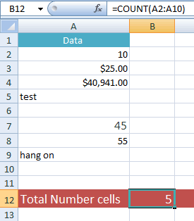
You can see, the COUNT function only returned the count for cells containing numbers. The blank and text cells are ignored while numbers with currency format are also included.
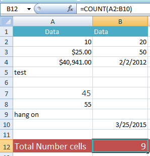
What if cells also contain dates?
The COUNT function also reruns the cells that contain dates. To demonstrate that, I extended the above range to B10 cell and added two numbers and two dates in B cells. So, the COUNT formula is:
=COUNT(A2:B10)
See the sheet figure with formula and result:
Using multiple ranges in COUNT function
Two things are further used in this formula. The first is using multiple ranges i.e. A2:A10 and C4:C8. The second thing tested whether COUNT function returns the text with number e.g. “6test”. See the formula and output:
=COUNT(A2:A10,C4:C10)
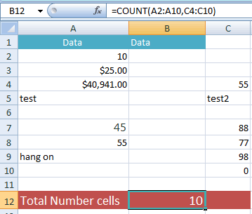
You saw, the COUNT did not return “2test” occurrence.
You may provide up to 255 ranges, cell references or items that you want to get the count.
Using Excel COUNTIF function for conditional counting
If you require getting the count of the number of cells based on single criteria then use the COUNTIF function. If you separate two words: “COUNT” “IF”, it makes the purpose clear.
For example, COUNT the cells from A2:D1000 IF that contains the word “Microsoft”. Similarly, return the number of cells which date is less than or equal to 10/10/2010 and so on.
General Syntax of COUNTIF:
=COUNTIF(Where to search, What to search)
You may provide a range of cells, array, names range etc as the first argument.
In “What to search” argument, you will specify e.g.
- “London”
- A cell reference like A10
- “>1” count the cells which value is greater than 1
- “<=10” less than or equal to 10
The next section shows a few examples of using the Excel COUNTIF function.
Getting the count of matched text
In this example, we will get the count of “Apple” in our example sheet. The column A cells contain the Fruits and Vegetable names. In the COUNTIF function, I specified the Apple as follows:
The result:
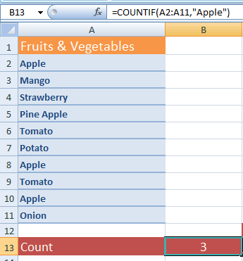
You can see the text Apple occurred three times in the given range.
Using the ‘*’ wildcard in COUNTIF function
You may also use the wildcards (* and ?) in the COUNTIF function. The ‘*’ is used for any sequence of characters while ‘?’ mark for the single character.
In the following example, I used the “to*” in the COUNTIF for the same sheet as used in above example and see the formula and result:
The COUNTIF formula:
The result:
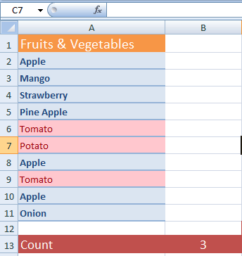
You saw the occurrences of Tomato (twice) and Potato (once) is returned as 3.
Using “>=” in COUNTIF for number count
For this example, I will use the single criteria for counting the cells containing the number of sales greater than or equal to 100 in the COUNTIF function.
For this example, the Excel sheet contains month names in B cells and number of sales in C cells. Following COUNTIF formula is used:
The resultant sheet:
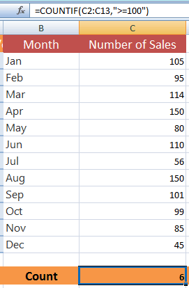
If you count the number of sales greater than or equal to 100, it is 6 that COUNTIF returned.
Using “<” operator in COUNTIF function
Now, we will get the count of Number of Sales less than 100 by using COUNTIF function. The following formula is used:
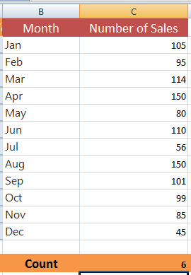
The count is again 6.
An example of Not equal to operator “<>”
For this example, I used the Not Equal to operator which is “<>”. The criterion set in the COUNTIF is to return the number of sales not equal to 150 i.e.
Result:
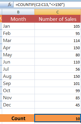
If you look at the data in the Excel sheet, it contains 150 twice. So, the COUNTIF omitted these and returned 10 counts.
Getting count of multiple ranges by COUNTIF
In this example, we will get the count of two different ranges by using COUNTIF function twice and adding the returned result.
For that, I have added another column in above sheet i.e. Amount. By using the COUNTIF function, we will get the count of (number of sales more than 100) + (Sale amount greater than or equal to $15000). See how this is translated into COUNTIF:
=COUNTIF(C2:C13,«>100»)+COUNTIF(D2:D13,«>=15000»)
The returned result:
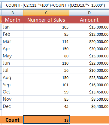
If you count the C cells (C2:C13) then the count of cells with more than 100 sales is 6. Add this to the count of D2:D15 cells with the amount greater or equal to 15000 then it is 7. The sum of both returned values is 13.
Note: Please do not mix it with using multiple conditions. The COUNTIF returned results separately and its result is summed. If we used minus operator then result would have been -1 i.e.
=COUNTIF(C2:C13,«>100») — COUNTIF(D2:D13,«>=15000»)
You may use more than two COUNTIF formulas as well. The function of using multiple conditions/criteria is COUNTIFS that is coming up in next sections.
The Example of using COUNTIF with dates
Just like the numbers, you may also write a criterion for date columns to get the count. For example, get the count of employees who joined after 3rd Jan 2012.
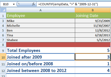
To demonstrate the usage of dates in COUNTIF function, I am using an Excel sheet containing fictitious records of employee names and their joining date. A named range is created which is referred to the COUNTIF function.
By using COUNTIF function, we will get the total count of employees, number of employees joined after 2010, the number of employees joined before 2007 and employees joined between 2008 to 2012. First, have a look at the resultant sheet which is followed by COUNTIF formulas:
The formula to get the total number of employees:
=COUNT(empData)
Where empData is the range name containing cells A3 to B7.
The COUNTIF formula for getting the number of employees joined after 2009:
=COUNTIF(empData, «>» & «2009-12-31»)
Joined on or before 2007:
=COUNTIF(empData, «<=» & «2007-12-31»)
Joined between 2008 to 2012 formula:
=COUNTIFS(empData,«>=»&«2007-01-01»,empData,«<=»&«2012-12-31»)
The last formula used COUNTIFS as we have two conditions to check. I will explain this in the COUNTIFS section.
You may learn more about the COUNTIF function in its tutorial: Using COUNTIF function.
An example of COUNTA function
If you require counting cells containing any type of data including numbers, text, empty string e.g. “”, dates, cells with error codes etc. then use the COUNTA function.
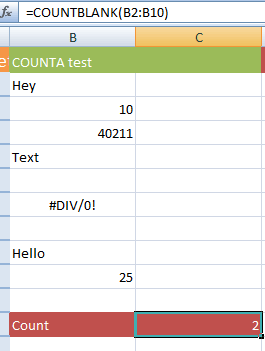
The COUNTA function will only omit the empty cells. See the following example, where I have used different types of values in Excel sheet and used COUNTA function for getting the count:
The COUNTA formula:
=COUNTA(B2:B10)
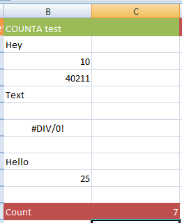
You can see, the resultant sheet displayed count as 7 as two cells in the given range are empty.
How to get the count of empty cells?
If you require the count of empty cells only then use the COUNTBLANK function. Have a look at the same Excel sheet and data as used for COUNTA function for demonstrating the COUNTBLANK function.
The Excel COUNTBLANK formula:
=COUNTBLANK(B2:B10)
The returned count is 2 as you can see the given range contains two blank cells.
How to use COUNTIFS function
As mentioned earlier, if you have multiple criteria to check for getting the count in a range, array etc. you may use the COUNTIFS function.
For example, return the count of those employees who joined after 10/20/2012 and their salary is $5000 or above. We have seen, the COUNTIF enables using single criterion only whereas COUNTIFS allows us getting the count based on above two criteria.
The example of using Excel COUNTIFS function
For the example of COUNTIFS function, I am using the same Excel sheet as used in an above example that contains Months, Number of Sales and Amount columns.
The requirement is to count those rows which Number of Sales is greater than or equal to 110 and amount >= $15000. The COUNTIFS formula is:
=COUNTIFS(C2:C13,«>=110»,D2:D13,«>=15000»)
The result:
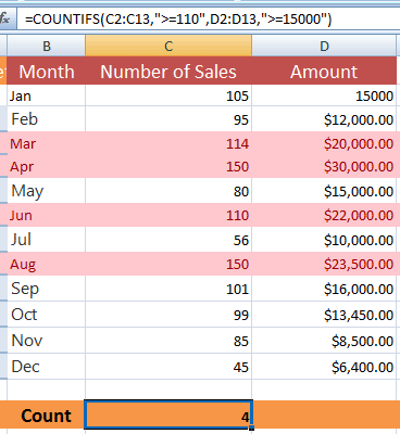
You can see, the highlighted rows met both criteria. If you look at the first row, the amount is $15000 that is true, however, the Number of sales is 105 which is False; so COUNTIFS did not include this row.
Using three conditions in COUNTIFS
You may use up to 127 range/criteria pairs in the COUNTIFS function. In this example, I am using three conditions in the COUNTIFS. For that, extending the above formula and another criterion is added to return the count of those rows that start with month “J”. While the number of sales is set as greater than 100.
The COUNTIFS formula:
=COUNTIFS(B2:B13,«J*»,C2:C13,«>100»,D2:D13,«>=15000»)
The result:
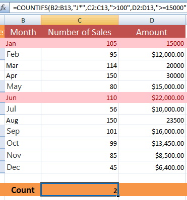
You see, I used ‘*’ wildcard as the first criteria i.e. B2:B13,”J*”. If you go through the table, only two highlighted rows met all the criteria given in COUNTIFS function.
October 28, 2020

Excel has a number of counting formulas that provide you great flexibility in summarizing data. There are many circumstances where it is helpful to count items in Excel. Sometimes you just want to know how many cells have “something” in them, whatever that something is. Other times, you want to know how many cells don’t have anything in them. Still other times you might want to count only cells that include specific text. Fortunately, Excel has many ways to help you count data. Let’s take a look at a few of the options available to you.
COUNT
=COUNT(range)
This formula counts the number of selected cells that contain numbers. It will ignore any cells that contain anything other than numbers for the purposes of counting. This would be helpful for counting the number of orders, for example, using the column with the final total of the order.
COUNTIF
=COUNTIF(range,criteria)
The COUNTIF function includes the cell in the count only if the contents of the cell match what you specify. An example of where I have used this function is counting replies for event attendance. I could have a spreadsheet with a column marked Attendance and then type Yes or No in the individual cells, as appropriate. Typically I would leave the fields blank to indicate someone has not responded yet (and use Conditional Formatting to turn those blank cells bright yellow, so they would stand out visually in a longer list of data). If I wanted to know the number of Yes responses in column B with a list of ten attendees, I would type the formula =COUNTIF($B$1:$B$10,”Yes”). Note that the criteria must be in double quotes. I could then copy that formula and change the Yes to No to find out how many people had declined the event invitation. I am using the dollar symbols in the formula to force Excel to only use those cells (known as absolute references) when I copy and paste the formula to a different cell.
COUNTIFS
=COUNTIFS(criteria range 1, criteria 1, criteria range 2, criteria 2,…).
The COUNTIFS function includes the cell in the count only if it matches what you specify, but the S added on the end of the function name allows you to specify more than one parameter. All criteria specified must be present in order for the cell to be counted, not just one of the criteria. An example of using this type of function would be counting the number of customers that had placed orders greater than $100,000 during the month of September. Additional criteria could be added, such as in a certain state or regional office location. You can specify up to 127 different criteria, though I confess, I can’t imagine having that many restrictions. The general format of the formula is to establish what the criteria range is and then what the criteria is. If I had 1000 orders and my Order Amount field in column D with my month of order field being in Column E, I would create the formulas as =COUNTIFS(D1:D1000,”>100000”, E1:E1000,”September”).
COUNTA
=COUNTA(range)
The COUNTA function will provide a count of selected cells that are not empty. Unlike the COUNT function, which only counted a cell if it had a number, COUNTA doesn’t care what the cell contains, as long as it is not blank. I would use this formulas to count the number of responses in a survey, for instance, where the results of each survey were typed in a separate row.
COUNTBLANK
=COUNTBLANK(range)
The COUNTBLANK function will count the number of selected cells that are empty. Using my earlier example of an event attendance list, this is a great way to know how many responses are outstanding, using the blank Attendance column cells.
I hope you enjoyed learning about these different COUNT functions that are built in to Excel. They can save you a lot of time and frustration.
About the Author:
Marie Herman CAP, OM, ACS, MOSM is the founder of MRH Enterprises LLC, whose services include teaching technology and professional development classes through corporate training and various webinars and workshops, writing articles, and more. She leads study groups to prepare students for Google G Suite, Microsoft Office Specialist, and the Certified Administrative Professional certification exams.
- Technology