
COUNTIF Not Blank Function
The COUNTIF not blank function counts non-blank cells within a range. The universal formula is “COUNTIF(range,”<>”&””)” or “COUNTIF(range,”<>”)”. This formula works with numbers, text, and date values. It also works with the logical operators like “<,” “>,” “=,” and so on.
Note: Alternatively, the COUNTA functionThe COUNTA function is an inbuilt statistical excel function that counts the number of non-blank cells (not empty) in a cell range or the cell reference. For example, cells A1 and A3 contain values but, cell A2 is empty. The formula “=COUNTA(A1,A2,A3)” returns 2.
read more can be used to count the non-blank cells.
Table of contents
- COUNTIF Not Blank Function
- How to Use COUNTIF Non-Blank Function?
- #1–Numerical Values
- #2–Text Values
- #3–Date Values
- The Characteristics of COUNTIF Not Blank Function
- Frequently Asked Questions
- Recommended Articles
- How to Use COUNTIF Non-Blank Function?
How to Use COUNTIF Non-Blank Function?
#1–Numerical Values
The steps to count non-empty cells with the help of the COUNTIF function are listed as follows:
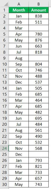
- In Excel, enter the following data containing both, the data cells and the empty cells.

- Enter the following formula to count the data cells.
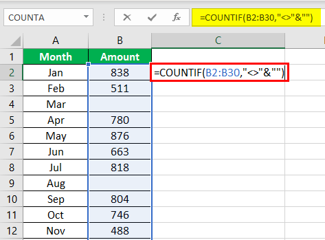
“=COUNTIF(range,”<>”&””)”
In the range argument, type B2:B30. Alternatively, select the range B2:B30 in the formula, as shown in the following image.

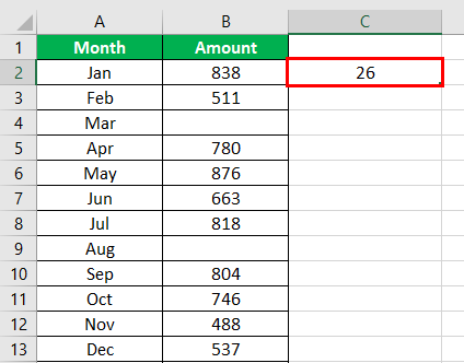
- Press the “Enter” key. The number of non-blank cells in the range B2:B30 appear in cell C2. The output is 26, as shown in the succeeding image.
This implies that there are 26 cells in the given range that contain a data value. This data can be a number, text, or any other value.

#2–Text Values
The steps to count non-empty cells within text values are listed as follows:
- Step 1: In Excel, enter the data as shown in the following image.
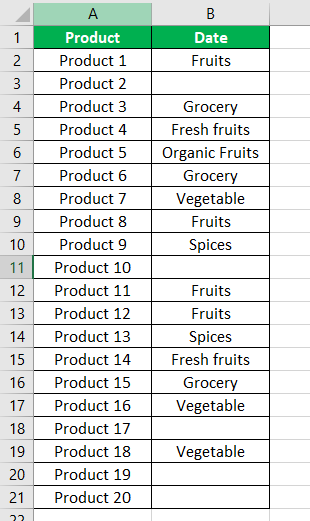
- Step 2: Select the range within which data needs to be checked for non-blank values. Enter the formula shown in the succeeding image.
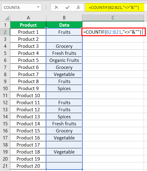
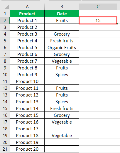
- Step 3: Press the “Enter” key. The number of non-blank cells in the range B2:B21 appear in cell C2. The output is 15, as shown in the succeeding image.
Hence, the COUNTIF not blank formula works with text values.
#3–Date Values
The steps to count non-empty cells, when the data consists of dates, are listed as follows:
- Step 1: In Excel, enter the data as shown in the following image. Select the range whose data needs to be checked for non-blank values. Enter the following formula.
“=COUNTIF(B2:B21,”<>”&””)”
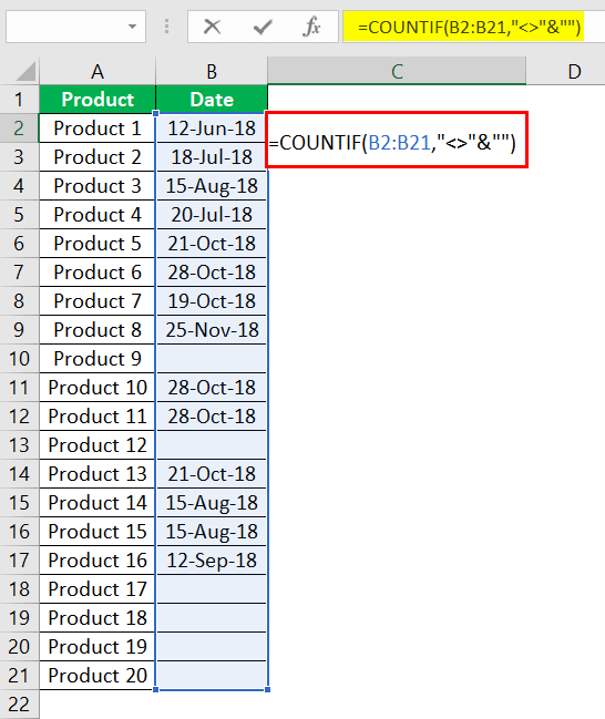
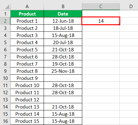
- Step 2: Press the “Enter” key. The number of non-blank cells in the range B2:B21 appear in cell C2. The output is 14, as shown in the succeeding image.
Hence, the COUNTIF not blank formula works with data that consists of date values.
The Characteristics of COUNTIF Not Blank Function
- It is case insensitive, implying that the output remains the same irrespective of whether the formula is entered in uppercase or lowercase.
- It works for data that consists of numbers, text, and date values.
- It works with greater than (>) and less than (<) operators.
- It is difficult to use the formula with long strings.
- The criteria (condition) must be specified within a pair of inverted commas to avoid errors.
Frequently Asked Questions
How is the COUNTIF formula used to count blanks?
The universal formula for counting blanks is stated as follows:
“COUNTIF(range,””)”
This formula works with all types of data values.
Note: Alternatively, the COUNTBLANK function can be used to count blank cells.
How does the COUNTIF function count the duplicate values?
The formula for counting the duplicate value is given as follows:
“COUNTIF(range,“duplicate value”)”
The “range” represents the range within which the duplicate values are to be counted. The “duplicate value” is the exact data value that is to be counted.
For example, to count the number of times the text “fruits” appears in the range A2:A10, we use “=COUNTIF(A2:A10,“fruits”).”
- The COUNTIF not blank function counts the non-blank cells within a given range.
- The generic formula of the COUNTIF not blank function is stated as–“COUNTIF (range,“<>”&””).”
- The criteria (condition) must be specified within a pair of inverted commas to avoid errors.
- The COUNTIF functionThe COUNTIF function in Excel counts the number of cells within a range based on pre-defined criteria. It is used to count cells that include dates, numbers, or text. For example, COUNTIF(A1:A10,”Trump”) will count the number of cells within the range A1:A10 that contain the text “Trump”
read more works for data that consists of numbers, text, and date values. - The COUNTIF formula gives the same output irrespective of whether the formula is entered in uppercase or lowercase.
Recommended Articles
This has been a guide to Excel COUNTIF not blank. Here we discuss how to use the COUNTIF function to count non-blank cells along with practical examples and a downloadable Excel template. You may learn more about Excel from the following articles –
- Not Equal in VBA
- COUNTIF with Multiple Criteria
- VLOOKUP Errors
- Use Not Equal to in Excel
- XML in Excel
Excel for Microsoft 365 Excel 2021 Excel 2019 Excel 2016 Excel 2013 Excel 2010 Excel 2007 More…Less
To count numbers or dates that meet a single condition (such as equal to, greater than, less than, greater than or equal to, or less than or equal to), use the COUNTIF function. To count numbers or dates that fall within a range (such as greater than 9000 and at the same time less than 22500), you can use the COUNTIFS function. Alternately, you can use SUMPRODUCT too.
Example
Note: You’ll need to adjust these cell formula references outlined here based on where and how you copy these examples into the Excel sheet.
|
1 |
A |
B |
|---|---|---|
|
2 |
Salesperson |
Invoice |
|
3 |
Buchanan |
15,000 |
|
4 |
Buchanan |
9,000 |
|
5 |
Suyama |
8,000 |
|
6 |
Suyma |
20,000 |
|
7 |
Buchanan |
5,000 |
|
8 |
Dodsworth |
22,500 |
|
9 |
Formula |
Description (Result) |
|
10 |
=COUNTIF(B2:B7,»>9000″) |
The COUNTIF function counts the number of cells in the range B2:B7 that contain numbers greater than 9000 (4) |
|
11 |
=COUNTIF(B2:B7,»<=9000″) |
The COUNTIF function counts the number of cells in the range B2:B7 that contain numbers less than 9000 (4) |
|
12 |
=COUNTIFS(B2:B7,»>=9000″,B2:B7,»<=22500″) |
The COUNTIFS function (available in Excel 2007 and later) counts the number of cells in the range B2:B7 greater than or equal to 9000 and are less than or equal to 22500 (4) |
|
13 |
=SUMPRODUCT((B2:B7>=9000)*(B2:B7<=22500)) |
The SUMPRODUCT function counts the number of cells in the range B2:B7 that contain numbers greater than or equal to 9000 and less than or equal to 22500 (4). You can use this function in Excel 2003 and earlier, where COUNTIFS is not available. |
|
14 |
Date |
|
|
15 |
3/11/2011 |
|
|
16 |
1/1/2010 |
|
|
17 |
12/31/2010 |
|
|
18 |
6/30/2010 |
|
|
19 |
Formula |
Description (Result) |
|
20 |
=COUNTIF(B14:B17,»>3/1/2010″) |
Counts the number of cells in the range B14:B17 with a data greater than 3/1/2010 (3) |
|
21 |
=COUNTIF(B14:B17,»12/31/2010″) |
Counts the number of cells in the range B14:B17 equal to 12/31/2010 (1). The equal sign is not needed in the criteria, so it is not included here (the formula will work with an equal sign if you do include it («=12/31/2010»). |
|
22 |
=COUNTIFS(B14:B17,»>=1/1/2010″,B14:B17,»<=12/31/2010″) |
Counts the number of cells in the range B14:B17 that are between (inclusive) 1/1/2010 and 12/31/2010 (3). |
|
23 |
=SUMPRODUCT((B14:B17>=DATEVALUE(«1/1/2010»))*(B14:B17<=DATEVALUE(«12/31/2010»))) |
Counts the number of cells in the range B14:B17 that are between (inclusive) 1/1/2010 and 12/31/2010 (3). This example serves as a substitute for the COUNTIFS function that was introduced in Excel 2007. The DATEVALUE function converts the dates to a numeric value, which the SUMPRODUCT function can then work with. |
Need more help?
Want more options?
Explore subscription benefits, browse training courses, learn how to secure your device, and more.
Communities help you ask and answer questions, give feedback, and hear from experts with rich knowledge.
In this example, the goal is to count cells that do not contain a specific substring. This problem can be solved with the COUNTIF function or the SUMPRODUCT function. Both approaches are explained below. Although COUNTIF is not case-sensitive, the SUMPRODUCT version of the formula can be adapted to perform a case-sensitive count. For convenience, data is the named range B5:B15.
COUNTIF function
The COUNTIF function counts cells in a range that meet supplied criteria. For example, to count the number of cells in a range that contain «apple» you can use COUNTIF like this:
=COUNTIF(range,"apple") // equal to "apple"
Note this is an exact match. To be included in the count, a cell must contain «apple» and only «apple». If a cell contains any other characters, it will not be counted. To reverse this operation and count cells that do not contain «apple», you can add the not equal to (<>) operator like this:
=COUNTIF(range,"<>apple") // not equal to "apple"
The goal in this example is to count cells that do not contain specific text, where the text is a substring that can be anywhere in the cell. To do this, we need to use the asterisk (*) character as a wildcard. To count cells that contain the substring «apple», we can use a formula like this:
=COUNTIF(range,"*apple*") // contains "apple"
The asterisk (*) wildcard matches zero or more characters of any kind, so this formula will count cells that contain «apple» anywhere in the cell. To count cells that do not contain the substring «apple», we add the not equal to (<>) operator like this:
=COUNTIF(range,"<>*apple*") // does not contain "apple"
The formulas used in the worksheet shown follow the same pattern:
=COUNTIF(data,"<>*a*") // does not contain "a"
=COUNTIF(data,"<>*0*") // does not contain "0"
=COUNTIF(data,"<>*-r*") // does not contain "-r"
Data is the named range B5:B15. The COUNTIF function supports three different wildcards, see this page for more details.
Note the COUNTIF formula above won’t work if you are targeting a particular number and cells contain numeric data. This is because the wildcard automatically causes COUNTIF to look for text only (i.e. to look for «2» instead of just 2). In addition, COUNTIF is not case-sensitive, so you can’t perform a case-sensitive count. The SUMPRODUCT alternative explained below can handle both situations.
With a cell reference
You can easily adjust this formula to use a cell reference in criteria. For example, if A1 contains the substring you want to exclude from the count, you can use a formula like this:
=COUNTIF(range,"<>*"&A1&"*")
Inside COUNTIF, the two asterisks and the not equal to operator (<>) are concatenated to the value in A1, and the formula works as before.
Exclude blanks
To exclude blank cells, you can switch to COUNTIFS function and add another condition like this:
=COUNTIFS(range,"<>*a*",range,"?*") // requires some text
The second condition means «at least one character».
See also: 50 examples of formula criteria
SUMPRODUCT function
Another way to solve this problem is with the SUMPRODUCT function and Boolean algebra. This approach has the benefit of being case-sensitive if needed. In addition, you can use this technique to target a number inside of a number, something you can’t do with COUNTIF.
To count cells that contain specific text with SUMPRODUCT, you can use the SEARCH function. SEARCH returns the position of text in a text string as a number. For example, the formula below returns 6 since the «a» appears first as the sixth character in the string:
=SEARCH( "a","The cat sat") // returns 6
If the text is not found, SEARCH returns a #VALUE! error:
=SEARCH( "x","The cat sat") // returns #VALUE!
Notice we do not need to use any wildcards because SEARCH will automatically find substrings. If we get a number from SEARCH, we know the substring was found. If we get an error, we know the substring was not found. This means we can add the ISNUMBER function to evaluate the result from SEARCH like this:
=ISNUMBER(SEARCH( "a","The cat sat")) // returns TRUE
=ISNUMBER(SEARCH( "x","The cat sat")) // returns FALSE
To reverse the operation, we add the NOT function:
=NOT(ISNUMBER(SEARCH( "a","The cat sat"))) // FALSE
=NOT(ISNUMBER(SEARCH( "x","The cat sat"))) // TRUE
We now have what we need to count cells that do not contain a substring with SUMPRODUCT. Back in the example worksheet, to count cells that do not contain «a» with SUMPRODUCT, you can use a formula like this
=SUMPRODUCT(--NOT(ISNUMBER(SEARCH("a",data))))
Working from the inside out, SEARCH is configured to look for «a»:
SEARCH("a",data)
Because data (B5:B15) contains 11 cells, the result from SEARCH is an array with 11 results:
{1;1;1;1;2;2;#VALUE!;#VALUE!;#VALUE!;#VALUE!;#VALUE!}
In this array, numbers indicate the position of «a» in cells where «a» is found. The #VALUE! errors indicate cells where «a» was not found. To convert these results into a simple array of TRUE and FALSE values, we use the ISNUMBER function:
ISNUMBER(SEARCH("a",data))
ISNUMBER returns TRUE for any number and FALSE for errors. SEARCH delivers the array of results to ISNUMBER, and ISNUMBER converts the results to an array that contains only TRUE and FALSE values:
{TRUE;TRUE;TRUE;TRUE;TRUE;TRUE;FALSE;FALSE;FALSE;FALSE;FALSE}
In this array, TRUE corresponds to cells that contain «a» and FALSE corresponds to cells that do not contain «a». This is exactly the opposite of what we need, so we use the NOT function to reverse the array:
NOT(ISNUMBER(SEARCH("a",data)))
The result from the NOT function is:
{FALSE;FALSE;FALSE;FALSE;FALSE;FALSE;TRUE;TRUE;TRUE;TRUE;TRUE}
In this array, the TRUE values represent cells we want to count. However, we first need to convert the TRUE and FALSE values to their numeric equivalents, 1 and 0. To do this, we use a double negative (—):
--NOT(ISNUMBER(SEARCH("a",data)))
The result inside of SUMPRODUCT looks like this:
=SUMPRODUCT({0;0;0;0;0;0;1;1;1;1;1}) // returns 5
With a single array to process, SUMPRODUCT sums the array and returns 5 as a final result.
One benefit of this formula is it will find a number inside a numeric value. In addition, there is no need to use wildcards to indicate position, because SEARCH will automatically look through all text in a cell.
Case-sensitive option
For a case-sensitive count, you can replace the SEARCH function with the FIND function like this:
=SUMPRODUCT(--NOT(ISNUMBER(FIND("A",data))))
The FIND function works just like the SEARCH function, but is case-sensitive. Notice we have replaced «a» with «A» because FIND is case-sensitive. If we used «a», the result would be 11 since there are no cells in B5:B15 that contain a lowercase «a». This example provides more detail.
Note: the SUMPRODUCT formulas above are more complex, but using Boolean operations in array formulas is a more powerful and flexible approach. It is also an important skill in modern functions like FILTER and XLOOKUP, which often use this technique to select the right data. The syntax used by COUNTIF is unique to a group of eight functions and is therefore not as useful or portable.
Want to learn more about how to count cells do not contain using Excel spreadsheet?? This post will give you an overview of how to use COUNTIF formula functions to get the number of cells that do not contain using Excel.
Syntax(Generic Formula)
=COUNTIF(range,”<>*txt*”)
How COUNTIF & COUNTIFS work
Excel has many syntax for a user who needs to specify on counting the total amount of cells with single or multiple criteria. For example, if you want to count cells based on more than one or more criteria, you can use the COUNTIF or COUNTIFS functions in Excel.
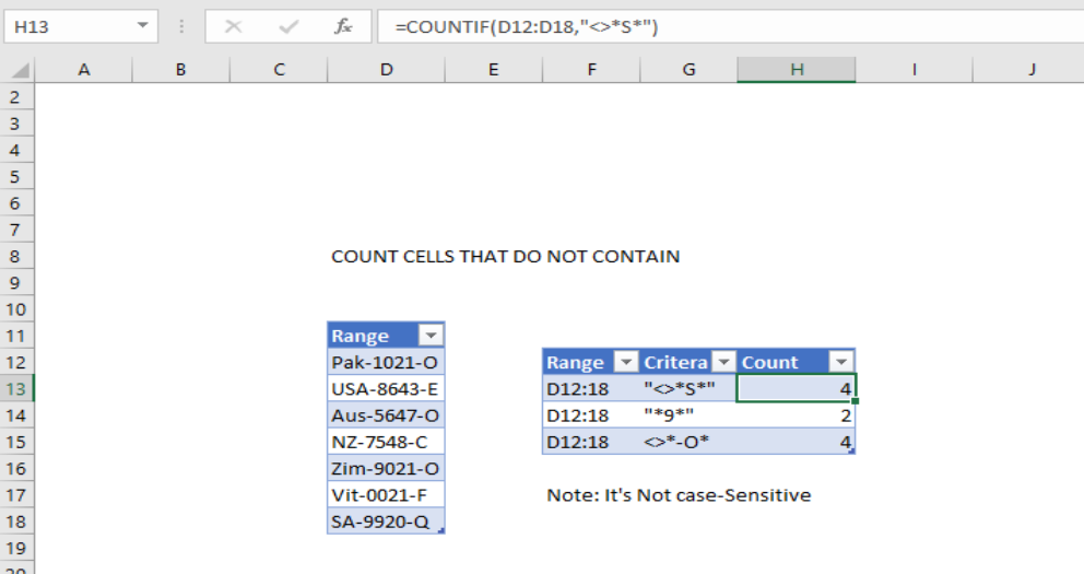 Figure 1: Example of count cells that do not contain
To count cells that do not contain, you can use the COUNTIF function. In the example shown, the formula in H13 is
=COUNTIF(D10:D18”<>”S”)
Difference Between COUNTIF & COUNTIFS
The difference between COUNTIF and COUNTIFS function is about the total number of condition that applies. While COUNTIF is designed to count the cells with a single condition, COUNTIFS function will let you have several criteria indifferent or in the same range as you wish.
=COUNTIFS(range”<>*?*”,rang”?*”)
By this tutorial, you have learned how to count the number of cells which don’t contain a specific text string.
Still need some help with Excel formatting or have other questions about Excel? Connect with a live Excel expert here for some 1 on 1 help. Your first session is always free.
In this article, we will learn about how to Count cells that do not contain value using COUNTIF function with wildcards in Excel.
In simple words, Consider a scenario in which we are required to count the data based on specific criteria in an array. counting cells that do not contain a specific value using wildcards to catch cell value with countif function in excel explained here with an example.
The COUNTIF function returns the count of cells that do not a specific value.
Syntax:
Range : array
Value : text in quotes and numbers without quotes.
<> : operator (not equal to)
Wildcard characters for catching strings and perform functions on it.
There are three wildcard characters in Excel
- Question mark ( ? ) : This wildcard is used to search for any single character.
- Asterisk ( * ): This wildcard is used to find any number of characters preceding or following any character.
- Tilde ( ~ ): This wildcard is an escape character, used preceding the question mark ( ? ) or asterisk mark( * ).
Let’s understand this function using it in an example.

There are different shades of colours in the array. We need to find the colours which do not have red.
Use the formula:
A2:A13 : array
<>*red* : condition where cells that don’t contain red in the cell value.

The red region marked are the 6 cells which do not contain red colour.
Now we will get the colours which do not have Blue
Use the formula:

There are 9 cells which do not have Blue.
Now we will get the colours which do not have Purple
Use the formula:
=COUNTIF(A2:A13,»<>*Purple*»)

As you can see the formula returns the count of cells which do not have a specific value.
Hope you understood how to use Indirect function and referring cell in Excel. Explore more articles on Excel function here. Please feel free to state your query or feedback for the above article.
Related Article:
How to Count Cells That Contain This Or That in Excel
How to Count Occurrences of a Word in an Excel Range in Excel
Get the COUNTIFS with Dynamic Criteria Range in Excel
How to Count total matches in two ranges in Excel
How to Count Unique Values In Excel
How To Count Unique Text in Excel
Popular Articles :
50 Excel Shortcut to Increase Your Productivity : Get faster at your task. These 50 shortcuts will make you work even faster on Excel.
How to use the VLOOKUP Function in Excel : This is one of the most used and popular functions of excel that is used to lookup value from different ranges and sheets.
How to use the COUNTIF function in Excel : Count values with conditions using this amazing function. You don’t need to filter your data to count specific values. Countif function is essential to prepare your dashboard.
How to use the SUMIF Function in Excel : This is another dashboard essential function. This helps you sum up values on specific conditions.